Sharif University of Technology
Scientia IranicaTransactions A: Civil Engineering http://scientiairanica.sharif.edu
A displacement nite volume formulation for the static
and dynamic analyses of shear deformable circular
curved beams
N. Fallah
and A. Ghanbari
Department of Civil Engineering, University of Guilan, Rasht, Iran.
Received 11 November 2015; received in revised form 28 May 2016; accepted 19 December 2016
KEYWORDS Curved beams; Finite volume; In-plane vibration; Membrane locking; Shear locking; Moving least squares.
Abstract. In this paper, a nite volume formulation is proposed for static and in-plane vibration analysis of curved beams in which the axis extensibility, shear deformation, and rotary inertia are considered. A curved cell with 3 degrees of freedom is used in discretization. The unknowns and their derivatives on cell faces are approximated either by assuming a linear variation of unknowns between the 2 consecutive computational points or by using the Moving Least Squares technique (MLS). The proposed method is validated through a series of benchmark comparisons where its capability in accurate predictions without shear and membrane locking deciencies is revealed.
© 2018 Sharif University of Technology. All rights reserved.
1. Introduction
The numerical modeling of the curved beams is a chal-lenging task due to the coexistence of three dierent load transfer mechanisms provided by the bending, shear, and membrane exibilities. The modeling of such coexistence of load carrying mechanisms may not be properly resolved, which leads to deciencies called as shear and membrane locking phenomena. These locking phenomena are seen in the nite element anal-ysis using two-node curved element with linear shape functions. Researchers have proposed various schemes to alleviate such deciencies, including reduced in-tegration [1], hybrid/mixed concepts [2], assumed displacement eld [3], use of algebraic trigonometric function [4], three-node curved beam element with trigonometric shape function [5], and use of discrete strain gap method [6]. Zhang and Di [7] presented accurate two-node nite element, which was derived
*. Corresponding author.
E-mail address: [email protected] (N. Fallah) doi: 10.24200/sci.2017.4259
from the potential energy principle and the Hellinger-Reissner functional principle. They introduced the internal displacement parameters for developing a high-order displacement-rotation interpolation eld. Kim and Kim [8] used the nodeless degrees of freedom tech-nique for developing an accurate, locking-free hybrid-mixed C(0) curved beam element.
Unlike the straight beams, the governing equa-tions of motion of curved beams are dependent not only on the rotation and radial displacement, but also on the coupled tangential displacement caused by the curvature of the structure. Wolf [9] employed straight elements to analyze the free vibration of elastic circular arcs ignoring the eects of shear deformation, but con-sidering rotary inertia eects. Irie et al. [10] calculated the natural frequencies of in-plane vibrations of circular curved beams with uniform cross-section where the eects of rotary inertia and shear deformation were considered. Eisenberger and Efraim [11] studied the uniform circular beams using the Timoshenko beam theory, which included the eects of rotary inertia, shear deformation, and the couplings of the radial and tangential displacements. Friedman and Kosmatka [12] utilized the Ritz method based on the trigonometric
functions and derived the exact static stiness matrix for the uniform circular curved beams. Yang et al. [13] used a four-node Lagrangian type curved beam element and a polynomial equation of order 5 describing the tangential displacement for modeling the uniform and nonuniform curved beams with variable curvatures.
All of the above-mentioned studies have been successfully applied to achieve the locking-free elements with dierent accuracy levels. Most of the formulations deal with two-node or three-node beam elements. However, it should be mentioned that higher accuracy of some of these elements is at the cost of inherent complex mathematical formulations.
In recent years, the Finite Volume (FV) tech-nique, which is a widespread and powerful technique in computational uid dynamics, has received a growing interest by the researchers for the solid mechanics anal-ysis. Elastic analysis of three-dimensional solids [14], stress analysis of elasto-plastic solids [15], bending analysis of elastic plates [16-18], dynamic of solids [19], dynamic uid-structure interaction [20], elasto-plastic analysis of plates [21], and active control of adaptive beams [22] are among the researches that expose the FV's capability in dealing with the variety of solid mechanics problems. FV formulations for the bending analysis of straight beams and plates have shown some advantages [17,18,21,22]; it is simple and transparent, it behaves well in the analysis of very thin to thick beams and plates, and it predicts accurate results without using any adjustable parameter for the analysis of thin beams and plates.
Two types of nite volume technique are common: cell vertex nite volume [14,17,19,20] and cell centered nite volume [15-18,21-24].
In this paper, the nite volume method is applied for the static and dynamic vibration analyses of shear-exible curved beams. Due to accounting for the transverse shear eects, the present formulation can be applicable for both thin and thick beams. For the nite volume analysis, rst, the beam is discretized into a mesh of curved elements known here as cells. For each cell, a computational point is considered at its center with three degrees of freedom. The internal forces act-ing on each cell are calculated and used in the balance equations of the cell. These equilibrium equations with equations expressing the boundary conditions provide a set of simultaneous linear equations, which can be solved for the unknown calculations. For the calcula-tion of the internal forces, the interpolacalcula-tion of unknown variables is needed, for which two approaches are used, namely, linear interpolation and interpolation based on the MLS technique. Although applying linear approach for the interpolation of unknowns in FV is common, however, using MLS approximation technique in FV is rather new. The MLS approximation technique has been known as a powerful technique in computer
graphics [25], however, it now becomes widespread and is used in mesh-free numerical methods for constructing shape functions.
To evaluate the proposed formulations, several numerical tests are performed, where no shear and no membrane lockings are observed in the analysis of Timoshenko curved beam models. Furthermore, the natural frequencies of some reference curved beams are calculated and the results are compared with the nite element and analytical results. Also, it is observed that using MLS increases the accuracy of the predictions.
This paper is presented in 6 sections. After Section 1, curved beam formulation based on the cell centered nite volume technique is presented in Section 2. Section 3 deals with the solution procedure for static and forced vibration analysis of curved beams. In Section 4, free vibration analysis of curved beams is presented. Section 5 deals with some benchmark tests, which are analyzed using the present formulation. Finally, in Section 6, we draw the conclusions.
2. Formulation
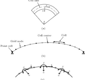
A portion of a circular curved beam is shown in Figure 1(a), which is discretized to a number of two-node curved elements along its centerline (Figure 1(b)). Each element is considered as a control volume or cell. In the cell centered nite volume approach, the computational points where the unknown variables are associated coincide with the centers of cells. Three degrees of freedom are assigned to each computational point, which are radial and tangential displacements
Figure 1. Discretization of a curved beam into the control volumes: (a) Curvilinear coordinate system, (b) discretized beam, and (c) degrees of freedom of the computational points.
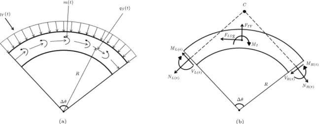
Figure 2. A generic internal cell with the dynamic loads: (a) External loads, and (b) internal loads.
and the cross-sectional rotation shown by w, u, and , respectively (Figure 1(c)).
To obtain the nite volume based formulation, it is needed to determine the governing static and dynamic equilibrium equations of each individual cell. A control volume under a time-dependent radial load is depicted in Figure 2. The internal forces and moment acting on both sides of the cell and the inertia forces are shown in this gure, where subscripts Ri and L denote the right and left sides of the cell, respectively. For the inplane dynamic analysis of the beam, the governing equations of motion of a typical cell shown above are as follows:
X
Mc(t) =0 ! MI
MRi(t) ML(t) (VR(t)
+ VL(t)) R tan2
= m(t)
+ 2qS(t)R2tg2 (1 cos2 ); (1)
X
FY(t) =0 ! FIY
(VRi(t) VL(t))
cos(
2 ) + (NRi(t) + NL(t)) sin
2
= 2qY(t)R sin2 ; (2)
X
FS(t) =0 ! FIS
(NRi(t) NL(t)) cos2
(VRi(t) + VL(t)) sin2
= 2qS(t)R sin2 ; (3)
where the terms with subscript I are the inertia-related terms following the D'Alembert principle; MI is the
inertia moment associated with angular acceleration around the axis normal to the plane of motion passing through the cell center; and FIS and FIY are also the
inertia forces corresponding to the linear accelerations in S and Y directions, respectively. It may be noted that the damping eects are neglected in the above equilibrium equations. is the included angle corresponding to the cell and R is its initial radius of curvature.
The internal forces and moments in the above equilibrium equations, acting on the cell faces, can be expressed in terms of the deformation-related terms using the constitutive equations [26]:
8 < :
M V N
9 = ;
j
= 2
4EI0 Ks0GA 00 0 0 EA
3 5
8 < :
d ds dw
dsdu+ + Ru ds wR
9 = ;
j
; (4) where j stands for the right and left faces of the cell, EI is the exural rigidity at the corresponding face, G is the shear modulus, A is the cross-sectional area of the corresponding face, Ks is the shear correction factor,
and R is the cell radius of curvature. Also, is the cross-sectional rotation, and u and w are displacements along the S and Y axes, respectively. All these displacement components correspond to the face j.
The displacement components as well as their gradients associated with both faces of the considered cell can be approximated in terms of displacement components measured at the centers of the considered cell and its neighboring cells. By using the interpola-tion techniques, which are explained in the following section, approximating Eq. (4), and substituting the results into Eqs. (1) to (3), one obtains:
MC
8 < :
w u
9 = ;
C
+ kC
8 < :
w u
9 = ;
C
where PC contains the external loads and matrix
MC is the diagonal mass matrix of the cell. The
acceleration terms, i.e. , w, and u, correspond to the considered cell center and the displacement terms that are gathered in the vectors of , w, and u are associated with the centers of the considered cell and its neighboring cells. Matrix kC contains the coecients
relating the unknowns associated with the considered cell and its neighboring cells. Depending on the utilized interpolation schemes, these intercell relations can be established.
Diagonal mass matrix MC contains the whole
mass of the cell, which is lumped at the cell center as:
MC=
2
4 m01 m02 00 0 0 m2
3
5 ; (6)
where m1is the mass moment of inertia and m2is the
total mass of the cell. m1 and m2 are obtained using
the following equations:
m1= I Si; m2= ASi; (7)
in which A, I, Si, and are cross-sectional area, inertia
moment, cell length, and volumetric mass density of the cell, respectively.
2.1. Interpolation
To calculate the unknown variables and their deriva-tives corresponding to the cell faces appeared in Eq. (4), two methods, namely, linear interpolation and MLS based interpolation, are used. These methods are explained in the following parts.
2.1.1. Linear interpolation
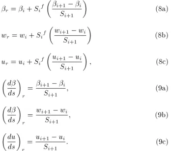
A typical internal cell, i, and its neighboring cells are shown in Figure 3. To calculate the unknowns and their required derivatives corresponding to the right face of the cell, i, which is a common face of cell i and cell i+1, a linear variation of unknown variables is assumed between the centers of the two neighboring cells. Thus, the unknown variables and their rst derivatives corresponding to that face can be calculated as [17,21,27]:
Figure 3. A generic internal cell and its neighboring cells.
r= i+ Sif
i+1 i
Si+1
(8a)
wr= wi+ Sif
wi+1 wi
Si+1
(8b)
ur= ui+ Sif
ui+1 ui
Si+1
; (8c)
d ds
r=
i+1 i
Si+1 ; (9a)
d ds
r
= wi+1 wi
Si+1 ; (9b)
du ds
r=
ui+1 ui
Si+1 : (9c)
Similar expressions can be written for the left face of the cell i. For a typical cell, C, substitution of Eqs. (8) and (9) into constitutive Eq. (4) provides results that can be used in Eqs. (1) to (3), leading to 3 equations in the form of Eq. (5).
Eq. (5) represents the relation of unknowns at the center of a cell with those at the centers of two neighboring cells. This procedure is applied for all the internal cells appearing in the model that provides three equations corresponding to each internal cell. 2.1.2. Higher order interpolation
The MLS method of interpolation is generally con-sidered to be one of the best schemes to interpolate random data with a reasonable accuracy because of its completeness, robustness, and continuity [28]. Accord-ing to the MLS, the distribution of a function u in can be approximated, over a number of scattered local points fsig (i = 1; 2; :::; n), as:
uh(s) = pT(s)a(s); 8s 2 ; (10)
where pT(s) = [p
1(s); p2(s); :::; pm(s)] is a monomial
basis of order m and a(s) is a vector containing coecients, which are functions of the coordinates [s1; s2; s3], depending on the monomial basis.
In the present study, the basis is chosen as: pT(s) =1; s; s2; s3; m = 4: (11)
The coecients included in vector a(s) are determined by minimizing a weighted discrete, L2, norm dened
as:
J(a(s)) =
N
X
I=1
WI(s)pT(sI)a(s) ^uI2
=pa(s) ^uITW
where sI denotes the position vector of node I, WI(s)
are the weighting functions, and ^uI are the nodal
parameters at s = sI. N is the number of nodes in
for which the weighting functions WI(s) > 0. One
may obtain the shape function as: uh(s) = 'T(s):^u =XN
I=1
I(s) ^uI; (13)
where:
'T(s) = pT(s)A 1(s)B(s); (14)
and its partial derivative is: 'I
;s= m
X
j=1
pj;s(A 1B)jI+pj(A;s1B + A 1B;s); (15)
where matrices A(s) and B(s) are dened by:
A(s) = pTWP = B(s)p =XN I=1
WI(s)p(sI)pT(sI);
(16)
B(s) =pTW =w
1(s)p(s1); w2(s)p(s2); :::::;
wN(s)p(sN)
: (17)
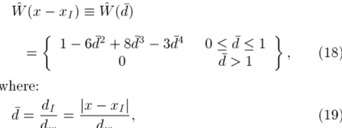
The weighting function in Eq. (12) denes the range of inuence of node I. Normally, it has a compact support. In the present study, N = 4 is considered and a quartic spline weighting function is used, which is:
^
W (x xI) ^W ( d)
=
1 6 d2+ 8 d3 3 d4
0 0 d > 1d 1
; (18) where:
d =ddI
w =
jx xIj
dw ; (19)
in which dI is the distance of node I from the sampling
point and dw is the size of the support domain for the
weighting function.
Support domain, s, is shown in Figure 4. As can
be seen in Figure 4, for the internal cells of a beam discretized to the uniform cells, the size of dwis 4 times
the length of the cells, while for the end point cells, the size of dwis 2 times the length of the cells. Eqs. (13) to
(15) can be used for approximating , w, and u as well as their derivatives corresponding to the right and left faces of each internal cell, which are required in con-stitutive Eq. (4). Then, the approximated concon-stitutive Eq. (4) is substituted in equilibrium Eqs. (1) to (3), which results in the discretized equilibrium equations in the form of Eq. (5). The above approximation procedure is applied for all the internal cells, which provides three equations corresponding to each internal cell.
Figure 4. Sub-domain for internal cell faces and point cells.
Figure 5. Point cells at the boundaries.
2.2. Boundary conditions
To introduce the boundary conditions to the solution procedure, point cells are used at the two ends of the beam (Figure 5). When displacement components are known at the end of the beam (displacement boundary condition), the incorporation of these known values in the solution procedure can be readily performed. Depending on the interpolation schemes used, we have the following equations for imposing the displacement boundary conditions; in case of using the linear inter-polations, we have:
8 < : w u 9 = ; Pb = 8 < : w u 9 =
;; (20)
and in case of using the MLS interpolation scheme, we have: 8 > > > > > > < > > > > > > : N P I=1 I(s) ^I N
P
I=1 I(s) ^wI N
P
I=1 I(s) ^uI
9 > > > > > > = > > > > > > ; Pb = 8 < : w u 9 =
; ; (21)
where asterisked values denote the known applied values and Pb indicates the point cell. When moment,
shear, and axial forces are known at the boundary (force boundary condition), we have:
MPb= M; VPb= V; NPb = N; (22)
where asterisked values denote the known applied values. Substituting constitutive equations with the approximated derivative expressions into the above equations gives the appropriate equations. For linear interpolation method, we have:
EI
Pb p
Sb
Pb
= M; (23a)
KsAG
(wPb wP)
Sb + Pb+
uPb
R
Pb
= V;
(23b)
EA
(uPb uP)
Sb
wPb
R
Pb
= N; (23c)
where the positive and negative signs are used for the right and left boundaries, respectively. Parameters with subscript Pb correspond to the point-cell at the
left or right boundary and parameters with subscript P correspond to the adjacent cell next to the point cell. When MLS interpolation scheme is used in the nite volume formulation, the force boundary conditions corresponding to a point cell, like the point cell at the left boundary, can be expressed in the following form:
EIb1;spb+ 2;s2+ 3;s3+ 4;s4cPn=M; (24)
KsAG
1;sWpb+ 2;sW2+ 3;sW3+ 4;sW4
+ 1pb+ 22+ 33+ 44
+ 1
R(1upb+ 2u2+ 3u3+ 4u4)
Pb
= V;
(25)
EA
1;supb+ 2;su2+ 3;su3+ 4;su4
1
R(1Wpb+ 2W2+ 3W3+ 4W4
Pb
= N;
(26) where parameters with subscripts 2, 3, and 4 are associated with the centers of the rst, second, and third neighboring cells, respectively. By applying the boundary conditions for the two point cells, three equations are obtained.
3. Solution procedure for the discretized equilibrium equations
Equations associated with all the internal cells and two point cells provide a system of simultaneous linear equations, which can be expressed in the matrix from: M X + TX = P; (27) where T contains the coecients relating the unknown variables and vector X contains the unknown variables. Vector P represents the known values on the bound-aries as well as the values that depend on the applied loads. Due to the sparse nature of T, Eq. (27) can be
solved by any appropriate solver technique for studying the bending behavior of the Timoshenko curved beam. In case of existence of damping eects, the above equation can be re-expressed as:
M X + C _X + TX = P; (28) where damping matrix C can be approximated using Rayleigh damping [29] as follows:
[C] = [M] + [K] ; (29) where and are the proportional damping constants, which are found using the following equation:
= 2 !m+ !n
!m!n
1
; (30)
where is the damping ratio, and !mand !n are
fre-quencies of two dierent modes [29]. After determining the mass, stiness, and damping matrices, it is possible to state the dynamic equation of the control volume. The set of equations of the whole cells gives a system of algebraic equations, which can be solved by applying an available solver technique. For solving the dynamic equilibrium in Eq. (27) or Eq. (28), the Newmark method with a constant acceleration assumption is used [29].
4. Free vibration
In order to study the harmonic vibrations of the beam, one can assume:
(s; t) = (s) sin !t; (31a) w(s; t) = w(s) sin !t; (31b) u(s; t) = u(s) sin !t; (31c) where ! is the frequency of the natural vibration mode of the curved beam. By substituting the above relations into Eq. (28), one can obtain the following eigenvalue equation:
KA = MA; (32)
where is the eigenvalue and A contains the natural modes of the vibrating beam.
5. Numerical results
To demonstrate the accuracy of the present formu-lations, some benchmark problems are studied and the results obtained are compared with the reference results reported in literature. At rst, the performance of the present formulation is evaluated for the analysis of some straight beam tests. For this purpose, the
present formulation, which corresponds to the curved beams, is adjusted by using a large value for the radius of curvature, R. It is aimed to demonstrate the capability of the present formulation for modeling the straight beams under static loads as well as to highlight the shear locking-free feature of the present method. 5.1. Uniformly loaded clamped-clamped
straight beam
As a rst evaluation test, the present formulation is used for the modeling of a uniformly loaded straight beam with the clamped-clamped boundaries. The material properties and geometry of the beam are L = 3 m, h = 0:3 m (depth), b = 0:01 m (width), q = 1 N/m, E = 2:1E11 N/m2, = 0:3, and K
s= 5=6. The
analytical prediction of the displacement at the middle of the beam span is calculated using the following equation given in Ref. [30]:
w
L 2
= qL4 384EI
1 + :96(1 + )h2 L2
: (33)
The beam is discretized by using an equally sized two-node element and, then, analyzed by the present method. The error of the predictions of the proposed approach is obtained as follows:
Error =wwfv 1 100; (34) where wfv is the predicted displacement and w is the
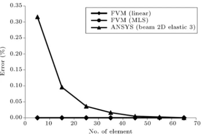
value calculated using Eq. (33). For modeling the straight geometry of the beam, a large value is used for the parameter R in the discretized equation (Eq. (27)). Figure 6 illustrates how the errors diminish as the number of elements is increased by mesh renement. The gure also shows that FVM with linear and MLS interpolation schemes predicts results that monoton-ically converge to the analytical solution. However, it may be noted that the results of FVM with MLS interpolation scheme converge to the corresponding analytical results faster than the FVM with linear interpolation technique.
Figure 6. Error in the prediction of mid-span displacement of a uniformly loaded clamped-clamped straight beam (L=h = 10).
Figure 7. The eect of aspect ratio, L=h, on the
prediction of mid-span displacement of a uniformly loaded clamped-clamped straight beam.
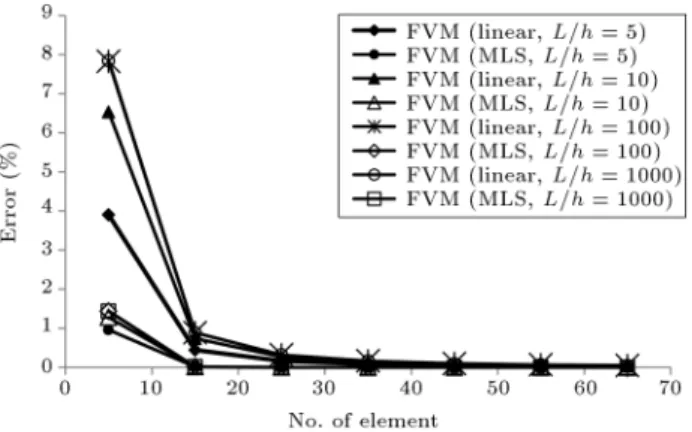
Also, in Figure 6, the results of the present method are compared with the results obtained by using ANSYS [31] software, in which the equally sized element type of Beam 2D-elastic3 is used for beam discretization. This element type is a two-node element with six degrees of freedom, which is able to model the shear eects. In order to have shear locking-free behavior, the reduced integration technique [32,33] is used in the element formulation. As Figure 6 shows, the predictions of the present method with either linear or MLS interpolation schemes are more close to the analytical value of Eq. (33) than the ANSYS predic-tions. To investigate the eect of aspect ratio, L=h, on the performance of the formulation, several aspect ratios, namely, 5, 10, 100, and 1000, are considered. The error in the prediction of mid-span transverse displacement is calculated corresponding to each aspect ratio. As Figure 7 demonstrates, the formulation is able to predict accurate transverse displacements of very thin to thick uniformly loaded clamped-clamped beams.
It is important to note that the shear locking phenomenon is not observed in the analysis of thin Timoshenko beam models. It is well known that to eliminate the shear locking deciency in the nite element analysis of Timoshenko beams, researchers have proposed techniques like reduced integration [32], selective integration [33], and some nite elements with rather complicated formulations [3,12,34].
5.2. Uniformly loaded cantilevered straight beam
The material properties, geometry, and load intensity of the beam are the same as those of the above test beam. FVMs with both linear interpolation and MLS interpolation are used for the analysis of the beam. Again, as we did in the above test, ANSYS with equally sized elements of Beam 2D-elastic3 is used for the analysis of the beam. The error in the predictions of the tip displacement is calculated relative to the values
Figure 8. Error in the prediction of tip displacement of a uniformly loaded cantilevered straight beam (L=h = 10).
given by [30]:
wtip= qL 4
8EI
1 + 0:8(1 + )Lh22
: (35)
Figure 8 illustrates the capability of the present formu-lation and ANSYS in dierent mesh densities, in which FVM shows remarkable capability. Also, to nd out the performance of the FVM in dealing with the uniformly loaded cantilevered beams of dierent thicknesses, several aspect ratios, namely, 5, 10, 100, and 1000, representing thick to very thin beams, respectively, are considered. The error in the prediction of tip transverse displacement is calculated corresponding to each aspect ratio. As shown in Figure 9, the formulation is able to predict accurate tip transverse displacement of cantilevered beams in the range of thick to very thin beams.
5.3. Cantilevered straight beam with tip transverse load
In this test, a cantilevered beam with a tip transverse load is concerned. This beam has been used in [35] for evaluating the capability of the proposed nite elements in dealing with the shear locking deciency.
Figure 9. Error in the prediction of tip displacement of a uniformly loaded cantilevered straight beam with dierent values of L=h.
The material properties and geometry of the beam are L = 4, h = 0:554256 (depth), b = 1 (width), E = 2:6 N/m2, = 0:3, and K
s = 0:85. The exact
tip transverse displacement, wT, is calculated using the
following relation taken from [36]: wT = P L
3
3EI
1 + 3EI KGAL2
: (36)
The tip displacement of the considered beam is ob-tained by using the nite volume method with both linear and MLS interpolation techniques, which are shown in Table 1. As mentioned above, this beam has already been studied in [35] by using the Timoshenko -nite element and a proposed higher order -nite element formulation. In that work, Timoshenko nite elements have been formulated using both full integration and reduced integration; however, full integration has been used in the formulation of the proposed higher order nite element. In Table 1, the results of FVM and those from [35] are given in which (wT F), (wT R),
and (wHOT) correspond to the results of Timoshenko
nite element with full integration, Timoshenko nite
Table 1. Comparison of displacements calculated by dierent approaches. No of
elements
WT F (FEM)
[35]
WT R (FEM)
[35]
WHOT (FEM)
[35]
FVM (linear)
FVM (MLS)
2 111.6 550.6 553.3 550.6 |
3 202.9 570.7 573.1 570.7 |
4 284.2 577.7 579.9 577.7 586.8
5 349.0 581.0 582.9 581.0 586.8
6 398.4 582.8 584.4 582.8 586.8
7 435.6 584.2 585.3 583.8 586.8
8 463.5 584.6 585.8 584.5 586.8
9 485.0 585.2 586.1 585.0 586.8
element with reduced integration, and higher order nite element with full integration, respectively. As can be seen, FVM with MLS interpolation predicts the analytical value by using only four elements. Also, FVM with linear interpolation produces results which monotonically converge to the analytical value. While the FVM with either interpolation is able to analyze this test beam, the results shown in the second col-umn of Table 1 indicate that the Timoshenko nite element formulation fails in accurate predictions due to shear locking phenomenon. To remove the shear locking defect in the Timoshenko nite element for-mulation, the reduced integration technique has been used. By using this technique, Timoshenko nite element predictions converge to the analytical results, as shown in the third column of Table 1. Also, the obtained results indicate that FVM with MLS interpolation converges faster than the higher order nite element formulation proposed by Heyliyer and Reddy [35].
5.4. A quarter circular cantilever ring
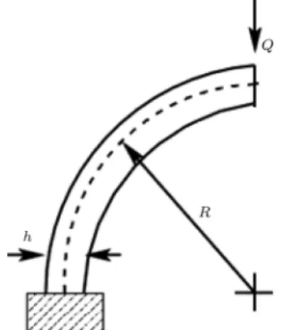
As the rst evaluation of the present formulation for the curved beam analysis, a quarter circular arc xed at one end and free at the other end is studied. As shown in Figure 10, the arc is subjected to a radial point force, Q = 1 kN at the free end, h = 1 m,
Figure 10. A quarter circular beam xed at one end.
E = 5:6E6 kN/m2, and G = 4E6 (kN/m2). Two
values of 10 and 50 m are assumed for R, which give the slenderness ratios, R=h, equal to 10 and 50, respectively. The ring is divided into the equal sized curved elements or cells and is analyzed by the present method. Also, the ring is modeled by ANSYS using two-node element of Beam 2D-elastic3, which is a straight element with six degrees of freedom. The dis-placement components at the free end are determined using both FV method and ANSYS, and then, the error of the predictions is calculated in comparison with the analytical values [3,7,34] calculated using Castigliano's energy theorem:
w = QR4EI3 +4GAK QR
s+
QR
4EA; (37)
u = 2EAQR + QR2EI3 2GAKQR
s; (38)
= QREI2: (39) Figures 11 to 13 depict the errors in the predictions for both arcs of R = 10 m and R = 50 m. It can be seen that both FV and ANSYS results monotically converge to the analytical values by increasing the element numbers. However, the FV predictions are more accurate than the ANSYS predictions when the same number of elements are used. It can be observed that even FV with linear interpolation predicts with more accuracy than the ANSYS.
5.5. A circular arc under dierent static loads This test concerns an arc with included angle of 120 degrees with dierent boundary conditions under the dierent loading scenarios, in total of 7 cases. The arc's properties are R = 4 m, opening angle = 2=3 (length l = 8=3), rectangular cross section with depth h = 0:6 and width b = 0:4 m, Young's modulus E = 30 GPa, and Poisson's ratio = 0:17. These arcs have already been used in the evaluation of the formulations proposed by Litewka and Rakowski [4]. The arc is analyzed by the present method as well as
Figure 12. Error in the prediction of end point tangential displacement.
Figure 13. Error in the prediction of end point sectional rotation.
by ANSYS using straight element Beam 2D-elastic3. The displacement components corresponding to the midpoint C are calculated and normalized as wc= wlc,
uc = ulc, and c = c, where l is the arc length and
is the arc opening angle.
The calculated results and the results of [4] are presented in Table 2.
It is observed that in all cases, except for the last one, the results of the FV with either linear or MLS interpolation techniques are found to be in good agree-ment with those reported in [4] and the predictions of ANSYS. In case 7, the results of FV and ANSYS are in good agreement, but far from the predictions reported in [4]. In that reference, the formulation of a two-node curved element has been developed by using the analytical shape functions of the trigonometric form. The element has been demonstrated to be shear and membrane locking-free; however, it does not perform properly in situations like case 7.
5.6. Free vibration of a curved beam (pinned-pinned)
A uniform circular beam with the pinned-pinned boundary condition is considered as another test to demonstrate the capability of the present formulation. The beam has already been studied in [13] with the following material and geometrical properties: R=r = 15, l=r = 23:56, ' = 90, R = 0:75 m, A = 4 m2,
I = 0:01 m4, E = 70 GPa, k
s = 0:85, ksG=E = 0:3,
and = 2777 kg/m3, where R, r =qI
A, l = R', and
are the radius of curvature, the radius of gyration, length of the curved beam, and the material density, respectively.
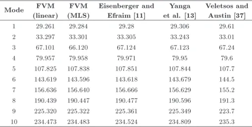
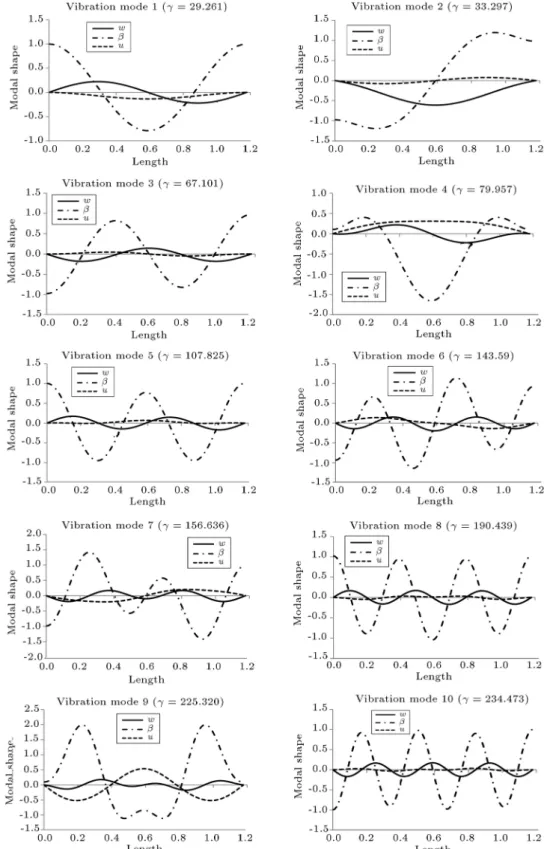
The non-dimensional natural frequencies ( = !l2qA
EI) of the rst 10 modes are calculated and
presented in Table 3. It is observed that very close agreement exists between the present results and those published in [11,13,36]. The associated modal shapes are also presented in Figure 14, where an excellent agreement is observed with the results given in [11]. It should be noted that in gures depicting the modal shapes, the horizontal axis represents the non-dimensional length parameter, s=l, in which s is the tangential curvilinear coordinate and l is the total length of the beam.
5.7. Free vibration of a curved beam (clamped-clamped)
In this test, a uniform circular curved beam with the clamped boundaries is studied. The geometrical and material properties are the same as those used in [13]: R=r = 15:915, l=r = 25, ' = 90, R = 0:6366 m, A = 1 m2, I = 0:0016 m4, E = 70 GPa, ks= 0:85, ksG=E =
0:3, = 2777 kg/m3.
The non-dimensional natural frequencies ( = !l2qA
EI) of the rst 10 modes are calculated and
presented in Table 4. The close agreement between the results of the present study and the reference results
Table 2. Normalized displacements at the center of a circular beam under dierent conditions. Case
no. Arc
Normalized displacement
Litewka and
Rakowski [4] ANSYS
FVM (linear)
FVM (MLS)
1 wC(10 6) 0.2488 0.2454 0.2485 0.2485
uC(10 6) 0.0000 0.0000 0.0000 0.0000
C(10 6) 0.0000 0.0000 0.0000 0.0000
2 wC(10 6) 0.0000 0.0000 0.0000 0.0000
uC(10 6) 0.1252 0.1202 0.1251 0.1251
C(10 6) 0.3796 0.374 0.3795 0.3794
3 wC(10 6) 0.0000 0.0000 0.0000 0.0000
uC(10 6) 0.0949 0.0936 0.0948 0.0949
C(10 6) 1.0824 1.0695 1.0819 1.0749
4 wC(10 6) 0.3047 0.2715 0.2806 0.2807
uC(10 6) 0.0000 0.0000 0.0000 0.0000
C(10 6) 0.0000 0.0000 0.0000 0.0000
5 wC(10 6) 0.0000 0.0000 0.0000 0.0000
uC(10 6) 0.2884 0.2833 0.2881 0.2883
C(10 6) 0.8064 0.8021 0.8064 0.8060
6 wC(10 6) 0.0000 0.0000 0.0000 0.0000
uC(10 6) 0.2016 0.2014 0.2015 0. 2016
C(10 6) 1.3613 1.3537 1.3612 1.3540
7 wC(10 6) 0.118 0.475 0.4722 0.4721
uC(10 6) 0.0000 0.0000 0.0000 0.0000
C(10 6) 0.0000 0.0000 0.0000 0.0000
Table 3. Non-dimensional frequencies, , of a uniform circular curved beam with the pinned-pinned boundary condition.
Mode FVM
(linear)
FVM (MLS)
Eisenberger and Efraim [11]
Yanga et al. [13]
Veletsos and Austin [37]
1 29.261 29.284 29.28 29.306 29.61
2 33.297 33.301 33.305 33.243 33.01
3 67.101 66.120 67.124 67.123 67.24
4 79.957 79.958 79.971 79.95 79.6
5 107.825 107.838 107.851 107.844 107.7
6 143.619 143.596 143.618 143.679 144.5
7 156.636 156.640 156.666 156.629 155.2
8 190.439 190.447 190.477 190.596 191.3
9 225.320 225.322 225.361 225.349 223.7
10 234.473 234.483 234.524 234.809 235.3
can be observed. The associated modal shapes are also presented in Figure 15, where an excellent agreement is observed with the results given by Eisenberger and Efraim [11].
For analyzing the above last two tests,
Eisen-berger and Efraim [11] have derived the nite element formulation using the shape functions, which are the exact solutions of the dierential equations of motion. Also, Yang et al. [13] have applied an element of 4 nodes with 12 degrees of freedom. However, in
Figure 14. Non-dimensional frequencies and vibration mode of a circular beam with uniform cross-section and pinned-pinned beam.
the proposed formulation, we use a curved cell of two points with three degrees of freedom in which even assuming a linear variation of unknowns be-tween the computational points can provide accurate results.
5.8. Forced vibration of a curved beam (clamped-clamped)
In this example, the forced vibration of a uniform circu-lar curved beam with the clamped-clamped boundary is studied (Figure 16). The geometrical and material
Figure 15. Non-dimensional frequencies and vibration mode of a circular beam with uniform cross-section and clamped-clamped boundary conditions.
Table 4. Non-dimensional frequencies of a uniform circular curved beam with the clamped-clamped boundary condition.
Mode FVM
(Linear)
FVM (MLS)
Eisenberger and Efraim [11]
Yanga et al. [13]
Veletsos and Austin [37]
1 37.705 36.704 36.703 36.65 36.81
2 42.268 42.267 42.264 42.289 42.44
3 82.239 82.237 82.233 82.228 82.5
4 84.494 84.494 84.491 84.471 84.3
5 122.311 122.310 122.305 122.298 122.5
6 154.949 154.949 154.945 154.998 155.1
7 168.208 168.208 168.203 168.174 167.7
8 204.479 204.478 204.472 204.599 {
9 238.998 238.997 238.992 238.973 {
10 248.019 248.016 249.011 249.320 249.6
Figure 16. Curved beam with the clamped-clamped boundary under dynamic load.
properties are R = 1 m, ' = 180, b = :05 m, h = 0:2 m, E = 200 GPa, ks= 0:85, = 0:3, and = 7850 kg/m3.
A uniformly distributed dynamic radial force of qY = sin t is applied to this curved beam, and
its radial vibration is studied. This beam is also analyzed by using ABAQUS [38] analysis tool, where the element B21 is applied for the discretization. In the B21 element formulation, the reduced integration technique is used for removing the locking deciency. For the dynamic analysis of the beam by the present formulation, the FVM with linear interpolation is used. The Newmark approach [29] is utilized for solving the dynamic equilibrium equation in which the parameters = 0:5 and = 0:25 are used. In Figure 17, the time history of radial displacement at the middle-span
Figure 17. Comparison of the time histories of radial displacement of middle-span of the arc between FVM and FEM methods.
Figure 18. Curved beam with the pinned-pinned boundary under the concentrated dynamic load.
of the beam is shown and compared with the results predicted by ABAQUS. The close predictions of both approaches are evident. This comparison demonstrates the capability of the proposed formulation for this dynamic analysis.
5.9. Forced vibration curved beam (pinned-pinned)
The uniform circular curved beam with the pinned-pinned boundary condition is considered as the last test problem (Figure 18). The beam has the following material and geometrical properties: R = 2 m, ' = 180, b = 0:05 m, h = 0:2 m, E = 200 GPa, ks= 0:85,
= 0:3, and = 7850 kg/m3.
A concentrated dynamic force of qY = sin t
is applied at the middle-span of the beam. Similar to the previous example, FVM with linear interpo-lation and the ABAQUS software are used for the analysis of the beam. The time histories of the radial displacement of the middle-span of the beam are obtained using both methods and compared with each other. Figure 19 shows the close predictions of both approaches.
6. Conclusions
In this work, the nite volume method presented in [23] and [27] has been extended for the modeling of the
Figure 19. Comparison of the time histories of the radial displacement of middle-span of the arc between FVM and FEM methods.
curved beams. The governing equations for the static and dynamic analyses have been simply obtained by studying the equilibrium of each individual cell, where the eects of the extensibility of the curved axis, the shear deformation, and the rotary inertia have been considered. For interpolation of unknowns, the linear approximation and MLS approximation schemes have been used. To evaluate the proposed approach, several benchmark tests has been studied. It has been demonstrated that the proposed formulation was able to model both curved beams and straight beams, where a large value for the radius of curvature is used for the straight beam models. In most test problems, MLS scheme has presented more accurate results than the linear interpolation scheme. The convergence of the solutions to the exact results in the static test cases showed that the proposed simple formulation is free of shear and membrane locking deciencies. Furthermore, the pro-posed approach has been applied to calculate the natural frequencies and analyze forced vibration of several curved beams, which had already been studied in the literature. Also, the comparison between the obtained results and the ref-erence results indicates the accuracy and eectiveness of the nite volume method for the vibration analysis of the curved beams. The attractive capabilities of the proposed approach in dealing with such rather challenging problem of curved beam models, even by using only 3 degrees of freedom for each cell (element), is promising.
References
1. Stolarski, H. and Belytschko, T. \Membrane locking and reduced integration for curved elements", J. Appl. Mech., 49(1), pp. 172-176 (1982).
2. Reddy, B.D. and Volpi, M.B. \Mixed nite element methods for the circular arch problem. Comput Meth-ods", Appl. Mech. Eng., 97(1), pp. 125-145 (1992). 3. Raveendranath, P., Singh, G., and Pradhan, B. \A
two-noded locking-free shear exible curved beam
element", Int. J. Numer. Meth. Eng., 44(2), pp. 265-280 (1999).
4. Litewka, P. and Rakowski, J. \The exact thick arc nite element. Comput Methods", Appl. Mech. Eng., 68, pp. 369-379 (1998).
5. Saari, H. and Tabatabaei, R. \A nite circular arch element based on trigonometric shape functions", Math Probl. Eng., Article ID. 78507, 19 pages (2007). DOI: 10.1155/2007/78507
6. Koschnick, F. and Bischo, M. \The discrete strain gap method and membrane locking", Comput. Methods Appl. Mech. Eng., 194, pp. 2444-2463 (2005). 7. Zhang, C. and Di, S. \New accurate two-noded
shear-exible curved beam elements", Comput. Mech., 30, pp. 81-87 (2003).
8. Kim, J.G. and Kim, Y.Y. \A new higher order hybrid mixed curved beam element", Int. J. Numer. Meth. Eng., 43, pp. 925-940 (1998).
9. Wolf, J.A. \Natural frequencies of circular arches", J. Struct. Eng.-ASCE, 97, pp. 2337-2350 (1971). 10. Irie, T., Yamada, G., and Tanaka, K. \Natural
fre-quencies of in-plane vibrations of arcs", J. Appl. Mech., 50, pp. 449-452 (1983).
11. Eisenberger, M. and Efraim, E. \In-plane vibrations of shear deformable curved beams", Int. J. Numer. Meth. Eng., 52, pp. 1221-1234 (2001).
12. Friedman, Z. and Kosmatka, J.B. \An accurate two-node nite element for shear deformable curved beams", Int. J. Numer. Meth. Eng., 41, pp. 473-498 (1998).
13. Yang, F., Sedaghati, R., and Esmailzadeh, E. \Free in-plane vibration of general curved beams using nite element method", J. Sound. Vib., pp. 850-867 (1998). 14. Bailey, C. and Cross, M. \A nite volume procedure to solve elastic solid mechanics problems in three dimensions on an unstructured mesh", Int. J. Numer. Meth. Eng., 38, pp. 1757-1776 (1995).
15. Demirdzic, I. and Martinovic, D. \Finite volume method for thermo-elasto-plastic stress analysis", Comput. Methods Appl. Mech. Eng., 109, pp. 331-349 (1993).
16. Wheel, M.A. \A nite volume method for analysing the bending deformation of thick and thin plates", Comput. Methods Appl. Mech. Eng., 147, pp. 199-208 (1997).
17. Fallah, N. \A cell vertex and cell centred nite volume method for plate bending analysis", Comput. Methods Appl. Mech. Eng., 193, pp. 3457-3470 (2004). 18. Fallah, N. \On the use of shape functions in the
cell centered nite volume formulation for plate bend-ing analysis based on Mindlin-Reissner plate theory", Comput Struct, 84, pp. 1664-1672 (2006).
19. Slone, A.K., Bailey, C., and Cross, M. \Dynamic solid mechanics using nite volume methods", Appl. Math. Modelling, 27, pp. 69-87 (2003).
20. Slone, A.K., Pericleous, K., Bailey, C., and Cross, M. \Dynamic uid structure interaction using nite vol-ume unstructured mesh procedures", Comput. Struct., 80, pp. 371-390 (2002).
21. Fallah, N. and Parandeh-Shahrestany, A. \A novel nite volume based formulation for the elasto-plastic analysis of plates", Thin Wall Struct., 77, pp. 153-164 (2014).
22. Fallah, N. and Ebrahimnejad, M. \Finite volume analysis of adaptive beams with piezoelectric sensors and actuators", Appl. Math. Model., 38, pp. 722-737 (2014).
23. Fallah, N. \Finite volume method for determining the natural characteristics of structures", J. Eng. Sci. Tech., 8(1), pp. 93-106 (2013).
24. Fallah, N. \A method for calculation of face gradients in two-dimensional, cell centred, nite volume formu-lation for stress analysis in solid problems", Sci. Iran., 15, pp. 286-294 (2008).
25. Lancaster, P. and Salkauskas, K. \Surfaces generated by moving least squares methods", Math. Comput., 37, pp. 141-158 (1981).
26. Day, R.A. and Potts, D.M. \Curved Mindlin beam and axi-symmetric shell elements - A new approach", Int. J. Numer. Meth. Eng., 30, pp. 1263-1274 (1990). 27. Fallah, N. and Hatami, F. \A displacement
formu-lation based on nite volume method for analysis of Timoshenko beam", In: Proceedings of the 7th International Conference in Civil Engineering, Iran, May 8-10 (2006).
28. Liu, G.R. and GU, Y.T., An Introduction to Mesh-free Methods and Their Programming, Springer Press, Berlin (2005).
29. Chopra, A.K., Dynamic of Structure, Theory and Applications to Earthquake Engineering, Prentice Hall (1995).
30. Majkut, L. \Free and forced vibration of Timoshenko beam described by single dierence equation", J. Theor. Appl. Mech., 47(1), pp. 193-210 (2009). 31. ANSYS, Swanson Analysis Systems Inc., Ansys
Refer-ence Manual (version 12.1) (2009).
32. Hughes, T.J.R., Cohen, M., and Haroun, M. \Reduced and selective integration techniques in the nite ele-ment analysis of plates", Nucl. Eng. Des., 46, pp. 203-222 (1978).
33. Bathe, K.J., Finite Element Procedures, Prentice-Hall (1996).
34. Lee, P.G. and Sin, H.C. \Locking-free curved beam element based on curvature", Int. J. Numer. Meth. Eng., 37(6), pp. 989-1007 (1994).
35. Heyliger, P.R. and Reddy, J.N. \A higher order beam nite element for bending and vibration problems", J. Sound. Vib., 126(2), pp. 309-326 (1998).
36. Prathap, G. and Bhashyam, G.R. \Reduced integra-tion and the shear-exible beam element", Int. J. Numer. Meth. Eng., 18, pp. 195-210 (1982).
37. Veletsos, A. and Austin, W. \Free vibration of arches exible in shear", J. Eng. Mech-ASCE, 99, pp. 735-753 (1973).
38. ABAQUS, 6.12.1.
Biographies
Nosrat-A. Fallah obtained his MSc degree from Isfahan University of Technology, Iran, in 1991, and PhD degree in Computational Structural Mechanics from the University of Greenwich, UK, in 2000, where he also worked as a Research Ocer. Then, he rejoined the Department of Civil Engineering at the University of Guilan, Iran, in 2002. Since that time, he has been mainly working on the development of the nite volume method for the modelling of various solid type problems, including geometrically non-linear problems and plate type structures. Recently, he has published papers concerning the meshless nite volume method, crack growth analysis, and adaptive renement in the meshless nite volume method for solid mechanics analysis. He is now Associate Professor in the Faculty of Civil Engineering of the Babol Noshirvani University of Technology.
Amir Ghanbary obtained his BSc degree in Civil Engineering in 2010 and his MSc degree in Structural Engineering from the University of Guilan in 2013. Mr. Ghanbary's thesis has concerned the development of a nite volume formulation for the static and dynamic analyses of curved beams.