Really?
by Wayne Ferson and
Yong Chen
First draft: April 25, 2012 This revision: February 24, 2015
ABSTRACT:
We refine an estimation-by-simulation approach to multiple hypothesis tests, recently applied to mutual fund performance by Barras, Scaillet and Wermers (BSW 2010). The model groups funds into negative, zero and positive-performance subgroups. We identify biases in the earlier approach, and find that the inferences about fund performance materially change. We use a sample of active US equity mutual funds, 1984-2011, and a sample of TASS hedge funds, 1994-2011. Our estimates indicate that smaller fractions of the funds have zero alphas, compared with previous evidence and methods. For mutual funds, the best fitting model implies two negative-alpha groups accounting for about half of the funds. For hedge funds we find that about half of the funds have negative alphas and nearly half are positive.
* Ferson is the Ivadelle and Theodore Johnson Chair of Banking and Finance and a Research Associate of the National Bureau of Economic Research, Marshall School of Business, University of Southern California, 3670 Trousdale Parkway Suite 308, Los Angeles, CA. 90089-0804, ph. (213) 740-5615, [email protected],
www-rcf.usc.edu/~ferson/. Chen is Associate Professor of Finance at Mays Business School, Texas A&M University, [email protected], ph: (979) 845-3870. We are grateful to Laurent Barras, Stéphane Chrétien, Danjiv Das, Chris Hrdlicka, Luke Taylor, and to participants at the 2013 Financial Research Association early ideas session, the 2014 Morgan Stanley Quantitative Equity Research Conference, the 2014 Financial Research Association, and workshops at Arizona State, Louisiana State, Melbourne, Miami, Santa Clara, Texas A&M, and a USC brown bag workshop for feedback.
1. Introduction
Imagine that the population of fund managers consists of three subpopulations, described in terms of their abnormal performance, or alphas 0,
g of “good” mangers have positive alphas centered at αg>0, and b are "bad" mangers with negative alphas, centered at αb<0. Barras, Scaillet and Wermers (BSW 2010) consider this problem and solve it by
simulating the cross-section of funds’ returns and using false discovery rate methods. A number of studies apply their approach to both mutual funds and hedge funds.1
BSW set αb = -3.2% and αg 0 = 75%
b = 24%, with data up to 2006. Their main estimates assume that the power of the tests is 100%, and that there is no chance that a bad fund (alpha<0) will be mistaken for a good fund (alpha>0) by the tests.
The model of BSW, in which mutual funds are members of one of three subpopulations, is appealing. Grouping is common when evaluating choices on the basis of quality that is multifaceted or hard to measure. For example, Morningstar rates mutual funds into “star” groups. Security analysts issue buy, sell and hold
recommendations. Academic journals are routinely grouped by quality, as are firms’ and nations’ credit worthiness. For investment funds, groups associated with zero, negative or positive alphas seems natural.
1 The False Discovery Rate is the expected fraction of the funds where the null
hypothesis of zero alphas is rejected, but for which the true alpha is zero. Cuthbertson et al. (2011) apply the BSW approach to UK mutual funds. Ardia and Boudt (2013) and Criton and Scaillet (2011) apply the method to hedge funds and Dewaele et al. (2011) apply it to funds of hedge funds. Romano et al. (2008) also present a small hedge fund example.
That some funds should have zero alphas is predicted by Berk and Green (2004). Under decreasing returns to scale, new money should flow to positive-ability managers until the performance left for investors is zero. There are also many reasons to think that some funds may have negative alphas. Most of these have to do with costs that keep investors from quickly pulling their money out of bad funds; such as taxes, imperfect information, agency costs and human imperfections such as the disposition effect, where investors for psychological reasons, hold on to their losing funds for longer than the economics would suggest. It is also natural to hope for funds with positive alphas, and these could be available because costs slow investors’ actions to bid them away. In the case of hedge funds, which we study in addition to mutual funds, there may be premiums in the alphas associated with compensation for lockup and notification periods (Aragon, 2007). A number of empirical studies find evidence that subsets of funds, identified through various means, may have positive alphas.
The approach here generalizes recent studies such as Kowsowski et al. (2006) and Fama and French (2010), who also bootstrap the cross-section of mutual fund alphas. In those studies, all of the inferences are conducted under the null hypothesis of zero alphas, so only one group of funds is modeled. The analysis is directed at the
hypothesis that all funds have zero alphas, accounting for the multiple hypothesis tests. The current approach also accounts for multiple hypothesis tests, but allows that some of the funds have nonzero alphas. Bootstrap simulations are conducted under the null and the alternative hypotheses in order to estimate the alpha values and the fractions of each type of fund in the population. We find that models with three subpopulations fit the cross-section of funds’ alpha t-ratios better than models in which there is only a
single group of funds with the same alpha.
We refine the approach of BSW by using more of the probability structure of the model. We allow for less than perfect power in the tests and allow for the possibility that a test will confuse a bad fund with a good fund, or vice versa. These
generalizations materially affect the results.
We show both analytically and with simulations that the assumption of perfect power in BSW leads to a bias toward finding too large a fraction of zero alpha funds. Using the same values that they use for the group alphas and a 5% size test, the power of the tests is in the 50-60% range – far below 1.0 -- and the BSW calculations produce estimates 0 that are severely biased. To illustrate, over our 1994-2011 sample period the BSW calculations suggest that about 90% of the hedge funds have zero alphas. In contrast, we estimate that most of the hedge funds’ alphas are nonzero. For mutual funds, BSW estimate that 75% have zero alphas. During our sample period their calculations suggest that more than 80% of mutual funds have zero alphas. Our estimates for mutual funds imply that 50% or fewer have zero alphas.
BSW report small standard errors for the fractions of good and bad funds, suggesting the ability to precisely estimate the actual fractions. For example (their Table II) the estimate of 24% bad funds has a reported standard error of 2.3%. We conduct simulation studies which suggest that their standard errors are consistent, but understated in finite samples. For example (in our Table 5), while the average reported standard error using the BSW calculations is 2.4%, the empirical standard error is really 4.1%. Because of the bias, the root mean squared error in the simulations is more than 28%. It makes sense that it should be more difficult to accurately estimate the fractions
of good and bad funds in the population than the BSW analysis suggests, in view of the notorious imprecision in the fund performance measures that both of our approaches rely on (e.g. Kothari and Warner, 2001).
We refine BSW further by simultaneously estimating both the true alphas and , such that simulated data drawn from the mixture produces estimates that most closely match the cross-section of alpha t-ratios we find in the actual data. BSW use a plug-in approach, fixing the true alpha parameters estimated in a separate step. Fixing the good and bad alpha values in a separate step may not provide accurate estimates of the fractions of funds in each subpopulation. Intuitively, if we set the true alphas to be too large, most funds will seem not have any performance. We find that inferences about the fractions of good and bad funds are sensitive to the values of the true alpha
parameters assumed, and we use the values that maximize the fit to the cross-section of fund alphas. The parameter values that we find are quite different from the values found by BSW for mutual funds.
We apply our approach to both active US equity mutual funds during 1984-2011 and a sample of hedge funds during 1994-2011. The best models mixing three alpha distributions implies that more than 50% of the hedge funds are “good,” with alphas centered around 0.2% per month, and most of the others are “bad,” with alphas
centered around -0.1% per month. For mutual funds, BSW used a good alpha of 0.317% per month and a bad alpha of -0.267%. The best models mixing three alpha
distributions for mutual funds implies that about 45% of the mutual funds are “good” (which here means zero alpha), about 5% are “bad” (alphas of -0.03% to -0.09% per
month) and the remaining half are “ugly” (alphas of -0.20 to -0.31% per month).2 We find many more negative alpha mutual funds and far fewer zero alpha funds than does the BSW method.
The basic probability model that we use assumes funds are drawn from one of three distributions centered at different alphas. In principle, the approach can be extended for many different alphas. However, in the three-alpha model joint
estimation reveals that there are linear combinations of the nonzero alpha values that produce a similar fit for the data, indicating that a three-group model is likely all that is needed, and perhaps simpler models with fewer groups might fit the data.
We estimate simpler models with only two alpha groups, one centered around zero and the other allowed to take either a positive or negative value. We also estimate models where there is a single alpha value around which all the funds are centered. In the two-group model the best-fitting nonzero alpha for mutual funds is negative, centered around -0.14% to -0.17% per month, and more than half of the funds have the negative alpha. The best-fitting nonzero alpha for hedge funds is positive, centered at 0.25% to 0.29% per month, and more than half of the hedge funds have the positive alpha. However, the two-group models do not fit the data as well as the three-group models. In the one-group models the single alpha for mutual funds is -0.21% to -0.22% per month, while for hedge funds it is 0.43% to 0.45% per month.
We also estimate the models on rolling, 60 month windows to examine the stability of the parameters over time, and we use each rolling window as a portfolio formation period to assess the information in the model about future fund returns. The
rolling window parameters show worsening performance over time for the good mutual funds and hedge funds, while the alphas of the bad funds are relatively stable over time. We find some evidence of potential investment value, but the spreads are relatively small. Much of the potential performance comes from identifying good hedge funds and avoiding bad mutual funds.
This paper is organized as follows. Section 2 describes our approach to the statistical problem. Section 3 describes the simulation details. Section 4 describes the data and Section 5 presents the empirical results. Section 6 provides a simulation analysis of the estimation-by-simulation parameter estimators and standard errors. Section 7 discusses robustness checks and Section 8 concludes. A short Appendix at the back describes our approach to the standard errors. An Internet Appendix relates our approach to previous studies, provides further analysis of the standard errors and presents ancillary results.
2. The Model
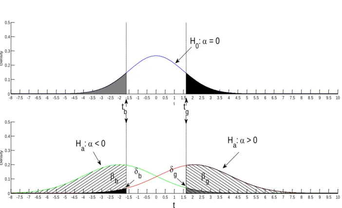
The basic structure of the probability model is illustrated in figure 1. We use three simulations to implement the approach. First, we set the size of the tests, say to 5%. Simulating the cross-section of mutual fund alphas under the null hypothesis that all of the alphas are zero produces two critical values for t-statistics, tg and tb. The critical value tg is the t-ratio above which 5% of the simulated t-statistics lie when the null of zero alphas is true. The critical value tb is the value below which 5% of the simulated t-statistics lie under the null hypothesis of zero alphas.
skill from luck. Our probability model with estimation by simulation draws a clear distinction between skill and luck. Funds that have no skill but produce t-ratios above the critical value for rejecting the null, are just lucky “false discoveries.” Our
probability model provides solutions for false discovery rates that refine previous studies and can be controlled by adjusting the size of the tests.3 We also control for cases of “unlucky” funds, which actually have positive alphas, but are found by the tests to have significant negative performance.
Our second step is to simulate the cross-section of alphas under the alternative hypothesis that managers are good, that is, the alphas are centered not at zero but around a value αg>0. The fraction of the simulated t-ratios above tg is the power of the test for good managers. This power, which we denote as βg, is assumed to be 1.0 in BSW. The fraction of the simulated t-ratios below tb is an empirical estimate of the probability of rejecting the null in favor of a bad manager when the manager is actually good. This “confusion” parameter, which we denote as δb, is assumed to equal zero in BSW. In fact, we find values of δb as large as 15% under some parameter values.4
A third simulation is based on the alternative hypothesis that managers are bad, that is, the alphas in the simulation are centered around a value αb<0. The fraction of the simulated t-ratios below tb is the power of the test for bad managers, βb. The fraction of the simulated t-ratios above tg is an empirical estimate of the probability of rejecting the null in favor of a good manager when the alternative of a bad manager is
3 The Internet Appendix derives the false discovery rates from our model, relates them to previous studies and applies the methods in a trading strategy.
4 Formally, δb is one corner of the 3 x 3 probabilistic confusion matrix characterizing the tests. See Das (2013, p.148) for a discussion.
true. This confusion parameter, which we denote as δg, is also assumed to equal zero in BSW. We find values of δg larger than 15% under some parameter configurations.
We combine the estimates as follows. Let Fb and Fg be the fractions of rejections of the null hypothesis in the actual fund data using the simulation-generated critical values, tb and tg. We model:
E(Fg) = P(reject at tg|H0 0 + P(reject at tg b + P(reject at tg g. (1) 0 + δg b + βg g, and similarly:
E(Fb) = P(reject at tb|H0 0 + P(reject at tb b + P(reject at tb g. (2) 0 + βb b + δb g.
b g, 0 =
1 - b - g) which we can solve given values of {δg , βg , δb , βb , Fg, Fb }. The solution to this problem is found numerically, by minimizing the squared errors of equations (1)
and (2) subject to the Kuhn- b g ≥0 and
b g ≤ 1. We estimate E(Fg) and E(Fb) by the fractions rejected in the actual data at the simulation-generated critical values, and we calibrate the parameters {δg , βg , δb , βb} from the simulations.
The Internet Appendix shows that our estimator of 0, derived by solving equations (1) and (2), reduces to the estimator from Storey (2002) used in BSW, when βg = βb =1 and δg = δb = 0. It also describes two offsetting biases in the BSW estimator. Assuming perfect power in the tests by setting βg = βb =1 bia 0 upwards, while assuming that the tests will never confuse a good and bad fund, by setting δg = δb = 0,
0 downwards. The net effect is an empirical question, which we answer with our bootstrap experiments. We find that the upward bias from assuming perfect power dominates, and the BSW estimator finds too many zero alpha funds.
The estimates of the π’s that result from equations (1) and (2) are conditioned on the values of {αg, αb}. We find that the estimates of the fractions can be sensitive to the values of the alphas assumed. Because the estimates of the population fractions are sensitive to the values of the alphas assumed, we refine the approach of BSW by
g,αb).
Our simultaneous estimation proceeds as follows. Each choice for the alpha
for the population of fund returns. We simulate data from the implied mixture of distributions, and we search over the choice of alpha values
estimates, until the simulated mixture distribution generates a cross-section of estimated fund alphas that best matches the cross-sectional distribution of alphas estimated in the actual data. The parameters that result are materially different from the values obtained using the BSW estimators.
The simulations are described in the next section, and the relation of our
approach to previous approaches of BSW and Storey (2002) are laid out in the Internet Appendix. A short Appendix at the end of the paper briefly describes how we get
, and the details are laid out in the Internet Appendix. In summary, our model generalizes the estimators of BSW in several important respects, by using more of the probability structure of the model. We avoid the
favor of finding too many zero alpha funds. This is important when the power of the tests is low, and low-power tests have long been seen as a problem in the mutual fund performance literature. We refine the separation of skill from luck by allowing for the possibility that the tests might be “confused,” finding a good (bad) fund which is really bad (good). Such confusion can occur when the location of good and bad funds is close together in the cross-section of test statistics. We simultaneously estimate the π
fractions, along with the location of good and bad funds in the distribution of fund alphas. We find materially different results about mutual fund alphas. Finally, we extend the analysis to hedge funds as well as mutual funds, and compare the results.
3. Simulation Details
We initially follow Fama and French (2010) when simulating under the null hypothesis that alpha is zero. We draw randomly with replacement from the rows of {rpt - αp, ft}t, where αp is the vector of alpha estimates in the actual data, rpt is the funds’ excess returns vector and ft is a vector of the factor excess returns. (Alternative approaches are considered in the robustness section.) All returns are excess of the one month return on a three month Treasury bill. This imposes the null that the “true” alphas are zero in the simulation. When we simulate under the assumption that the true alphas are not zero for a given fraction of the population, π, we select Nπ funds, where N is the total number of funds in the sample, and add the relevant value of alpha to their returns net of the estimated alpha, for the simulations. (An alternative approach is considered in the robustness section.) Each trial of the three simulations delivers an estimate of the δ and β parameters. We use and report the average of these across the 1,000 trials.
Our approach does not assume that a good or bad fund can only have a single value of alpha; instead, it is consistent with the assumption that the good and bad alphas are random and centered around the values (αg, αb).5
Fama and French use an 8-month survival screen for getting alpha estimates, arguing that the 60-month survival selection in BSW leads to biased results.6 We follow Fama and French to use an 8-month survival screen for mutual funds (12 months for the hedge funds). We impose the selection criterion only after a fund is drawn for an
artificial sample. This raises the issue of a potential inconsistency in the bootstrap, as the missing values will be distributed randomly through “time” in the artificial sample, while they tend to occur in blocks in the original data. This will produce an
inconsistency if there is serial dependence in the data. However, in fund return data we are much more concerned with cross-sectional dependence, which the simulations do preserve, than we are with serial dependence, which is very small in monthly returns. We do not think this problem is a material issue for our study.
While we describe the results in terms of the alpha values, all of the simulations are conducted using the t-ratios for the alphas as the test statistic, where the standard errors are the White (1980) heteroskedasticity consistent standard errors. We use the t-ratio because it is a pivotal statistic, which should improve the properties of the
5 Suppose, for example, that in the simulation we drew for each good fund a random true alpha, αpTRUE, equal to αg plus mean zero independent noise. In order to match the sample mean and variance of the fund’s return in the simulation to that in the data, we would reduce the variance of {rpt - αpTRUE}, by the amount of the variance of the noise in αpTRUE around αg . The results for the cross-section would come out essentially the same.
6 Dewaele et al. (2011) also use a 60-month survival screen, while Criton and Scaillet (2011) use a 36 month screen. BSW also use a 36 month screen in their appendix and
bootstrap compared with simulating the alphas themselves. An overview of the bootstrap is provided by Efron and Tibshirani (1993).
When we simulate the mixture of distributions for joint estimation we require a goodness-of-fit criterion to compare the alphas from the simulated mixture to the empirical distribution of alphas. We choose the familiar Pearson χ2 statistic as the criterion:
Pearson χ2 = Σi (Oi – Mi)2/Oi, (3)
where the sum is over K cells, Oi is the frequency of t-statistics for alpha that appear in cell i in the original data, and Mi is the frequency of t-statistics that appear in cell i using the model, where the null hypothesis is that the model frequencies match those of the original data. We choose K=100 cells, with the cell boundaries set so that an
approximately equal number of t-ratios for the alphas of funds in the original data appear in each cell (i.e., Oi ≈ N/100).7
4. The Data
We study mutual fund returns measured after expense ratios and funds’ trading costs, for 1984-2011 from the Center for Research in Security Prices Mutual Fund database,
report similar results to the 60-month screen.
7 BSW pick the alpha parameters for the groups by relaxing the assumption that the power of the tests is 100%. They compute the power from a noncentral t-statistic under alternative alpha values, and choose the alpha parameters to match the expected
fractions of skilled and unskilled funds found by simulation at those true alpha values, with the fractions of skilled and unskilled funds implied by the noncentral
t-distribution. These alpha values are plugged in to estimate the final fractions. Given that the fund return data are unlikely to precisely match the t-distribution, we prefer our simultaneous approach.
focusing on active US equity funds. We subject the mutual fund sample to a number of screens to mitigate omission bias (Elton Gruber and Blake 2001) and incubation and back-fill bias (Evans, 2010). We exclude observations prior to the reported year of fund organization, and we exclude funds that do not report a year of organization or which have initial total net assets (TNA) below $10 million or less than 80% of their holdings in stock in their otherwise first eligible year to enter our data set. Funds that
subsequently fall below $10 million in assets under management are allowed to remain, in order to avoid a look-ahead bias. We combine multiple share classes for a fund, focusing on the TNA-weighted aggregate share class.8 These screens leave us with a sample of 3716 mutual funds with at least 8 months of returns data.
Our hedge fund data are from Lipper TASS. We study only funds that report monthly net-of-fee US dollar returns, starting in January of 1994. We focus on US Equity oriented funds, including only those categorized for a given month as either Dedicated Short bias, Event driven, Equity market neutral, Fund-of-funds or
Long/short equity hedge. We require that a fund have more than 10 million US dollars in assets under management as of the first date the fund would otherwise be eligible to be included in our analysis.
To mitigate backfill bias, we remove the first 24 months of returns and returns before the dates when funds were first entered into the database, and funds with
8 We identify and remove index funds both by Lipper objective codes (SP, SPSP) and by searching the funds’ names with key word “index.” Our funds include those with
Policy code (1962-1990) CS, Wiesenberger OBJ (1962-1993) codes G, G-I, G-I-S, G-S, G-S-I, G-S-I, IFL, I-S, I-G, I-G-S, I-S-G, S-G, S-G-G-S-I, S-I-G, GCG-S-I, IEQ, LTG, MCG, SCG, Strategic Insight OBJ code (1993-1998) AGG, GMC, GRI, GRO, ING, SCG, Lipper OBJ/Class code (1998-present), CA, EI, G, GI, MC, MR, SG, EIEI, ELCC, LCCE, LCGE, LCVE, LSE,
missing values in the field for the add date. Some hedge funds may have returns data before the add date because they switch vendors. For example, a fund may first report to Hedge Fund Research and later switch to TASS for reasons unrelated to past
performance.
There is some evidence that younger hedge funds perform better. If that is true, we could be inappropriately screening out better performing young fund data, creating a bias against finding good hedge funds. This is a conservative bias in view of our finding that there are significantly more good hedge funds than there are mutual funds. For example, our data screens leave us with a sample of 3865 hedge funds with at least 8 months of returns data.9 If we do not screen out the first 24 months the number would be 4451. Suppose all of the screened funds were actually good funds. We estimate the fraction of good hedge funds to be about 52%. The correct value could then be as large as [0.52(3865) + (4451-3865)]/4451 = 58%. On the other hand, if all of the screened out funds were truly bad our estimate of the fraction of bad funds, which is about 45%, could be as large as [0.45 (3865) + (4451-3865)]/4451 = 52%. These
differences are within one standard error in magnitude.
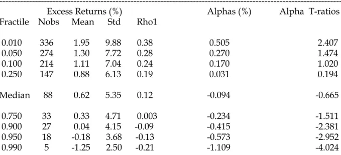
Table 1 presents summary statistics of the mutual fund and hedge fund data. The mean hedge fund return (0.37% per month) is smaller than the average mutual fund return (0.62%), but the longer sample for the mutual funds includes the high-return 1984-1993 period. The range of average high-returns across funds is much greater in
MCCE, MCGE, MCVE, MLCE, MLGE, MLVE, SESE, SCCE, SCGE, SCVE and SG.
9 For some of the subsequent analyses we impose a minimum 12-month data screen on the hedge funds, given the larger number of factors in their factor models. The
summary statistics are very similar, except that the alphas and t-ratios are less extreme in the 1% tails than shown in Table 1.
the hedge fund sample, especially in the negative-return, left tail. A larger fraction of the hedge funds lose money for their investors, and the losses have been larger than in the mutual funds.
The two right hand columns of Panel A of Table 1 summarize the Fama-French (1996) three-factor alphas and their heteroskedasticity-consistent t-ratios for the mutual funds. For the hedge funds in Panel B, we use the Fung and Hsieh (2001, 2004) seven factors. The Internet Appendix shows the results for hedge funds when the Fama and French factors are used.10
The median alpha for the hedge funds is positive, while for the mutual funds it is slightly negative. The tails of the cross-sectional alpha distributions extend to larger values for the hedge funds. For example, the upper 5% tail value for the t-ratio of the alphas in the hedge fund sample is 4.18 (the alpha is 1.25% per month), while for the
10 The hedge fund alphas are slightly smaller on average and the cross-sectional
distribution of the alphas shows thinner tails when the Fama and French factors are used. The Fung and Hsieh seven factors include the excess stock market return and a “small minus big” stock return similar to the Fama and French factors, except
constructed using the S&P 500, and the difference between the S&P500 and the Russell 2000 index. In addition, they include three “trend-following” factors constructed from index option returns; one each for bonds, currencies and commodities. Finally, there are two yield changes; one for ten-year US Treasury bonds and one for the spread between Baa and ten-year Treasury yields. Note that yield changes are not excess returns, which means that the factor model regression intercept is not strictly
interpretable as an excess return alpha. However, in the present context the error is likely to be negligible. Approximate the return on a bond benchmark as RB ≈ -D ∆y + c, where c is the coupon yield, D is the bond duration and ∆y is the yield change. If c≈Rf, the short term risk-free return, then the bond benchmark excess return that we should use on the right hand side of the regression is rB ≡ RB – Rf ≈ RB – c ≈ -D ∆y. Therefore, a regression of a fund’s excess return on the yield change produces a slope coefficient equal to -D times the coefficient on rB, and the fitted contribution to the expected return of the fund – the product of the slope and the mean of the right hand side variable - is approximately the same as if rB had been used.
mutual funds it is only 1.47 (the alpha is 0.27%). Thus, using conventional statistical standards and ignoring the multiple hypothesis test problem, it would seem that there are significantly skilled hedge funds, as well as negative alpha hedge funds, but
perhaps not many skilled mutual funds. In the left tails the two types of funds also present different alpha distributions, with a thicker lower tail for the alphas and t-ratios in the hedge fund sample. One of our goals is to see how these impressions of
performance hold up when we consider multiple hypothesis testing, and use
bootstrapped samples to capture the correlations and departures from normality that are present in the data.
Table 1 shows that the sample volatility of the median hedge fund return (2.62% per month) is smaller than for the median mutual fund (5.34%). The range of volatilities across the hedge funds is greater, with more mass in the lower tail. For example,
between the 10% and 90% fractiles of hedge funds the volatility range is 1.2% - 6.7%, while for the mutual funds it is 4.2%-7.0%. Getmansky, Lo and Makarov (2004) study the effect of return smoothing on the standard deviations of hedge fund returns and show that smoothed returns reduces the standard deviations and induces positive autocorrelation in the returns. The autocorrelations of the returns are slightly higher for the hedge funds, consistent with more return smoothing in the hedge funds. The
median autocorrelation for the hedge funds 0.16, compared with 0.12 for the mutual funds, and some of the hedge funds have substantially higher autocorrelations. The 10% right tail for the autocorrelations is 0.50 for the hedge funds, versus only 0.24 for the mutual funds. Asness et al. (2000) show that return smoothing can lead to
smoothing in the robustness section and in the Internet Appendix, and conclude that smoothing is not likely to be material for our results.
5. Empirical Results 5.1 Mutual Funds
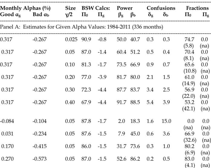
Table 2 presents some initial results for mutual funds, where the alphas are estimated using the Fama and French (1996) three-factor model. We check the sensitivity to this choice in the robustness section. The fractions of managers in the population with specified values of their true alphas, which are either zero, good or bad, are estimated using simulation. We use 1,000 simulation trials.
In the first five rows of Panel A of Table 2 we set the good and bad alphas equal to the values specified by BSW and vary the size of the tests. The second and third columns show the π fractions using the BSW estimators. In our sample period with γ/2 = 0.05 their calculations lead to π0 = 87.0% and πg = -1.4%.11 When the test size is 10% their estimators say π0 = 83.1% and πg = -1.7%. These π0 values are larger than the 75% value obtained by BSW, perhaps due to differences in the sample periods in our two studies. Their estimator for π0 is biased upwards, to a greater extent if the size of the tests γ/2 is small, and Table 2 shows that as γ/2 increases their calculations produce smaller π0 values -- as low as 67.9%when γ/2 = 0.40. Interpolating, we obtain a value close to their 75% value when γ/2 is about 0.25.
The Internet Appendix shows analytically that the bias in the BSW estimator of
11 The negative values arise in the BSW calculation because the fraction rejected Fg is smaller than (γ/2) π0. Our simultaneous approach, using constrained optimization, avoids the problem of negative probabilities.
π0 depends on the power of the tests and the confusion parameter. Their estimator assumes that the power is 100% and that the confusion is zero. When the power is below 100%, the estimator is biased upwards, finding too many zero alpha funds, while positive confusion biases the estimate downwards. Table 2 shows that the empirical power varies from about 50% to just over 90% as the size of the tests is increased, while the confusion parameters are 5.4% or less. Our approach delivers smaller estimates for the fractions of zero alpha funds than the BSW estimators. This reflects the fact, which we establish by simulation below, that the upward bias from assuming perfect power dominates the downward bias from assuming zero confusion in the BSW estimator.
The results in Table 2 suggest that a larger fraction of the mutual funds have negative alphas than BSW infer. For example, in their Table II, 9.8%-18.2% of the mutual funds are estimated to have negative alphas, depending on the size of the test. Of course, the sample periods in the two studies differ. During our sample period, Table 2 indicates that the BSW estimators say that 9.9% to 34.5% of the alphas are negative. Using our estimators, the first six rows of Table 2 say that 25.3% to 46.8% of the funds have negative alphas, using the same values for the true alpha parameters as used in BSW. These different results, which control for differences in the sample period, are explained by allowing the power parameters, β, to be less than 1.0 and allowing the confusion parameters, δ, to be greater than 0.0 in our general model. The standard errors for the π fractions in Table 2, shown in parentheses, are much larger than those reported by BSW. Our standard errors account for the
dependence of the tests across funds, which their calculations assume is zero (see the analyses in the Appendix), and which increases the standard errors. Our simulation
evidence, discussed below, finds that the BSW standard errors are understated in the finite samples used here. The standard errors reported in Table 2 are the empirical standard errors from our bootstrap simulations described below.
BSW recommend using large test sizes in order to have sufficiently high power to justify the assumption that the power is 100%. Larger γ/2 values, of course, do produce tests with higher power; for example, we find 91.7% and 88.5% power in the two tails when γ/2 = 0.40. However, at larger sizes the error rates δ, which BSW assume equal zero, become larger. In addition, as Table 2 illustrates, the standard
errors of the fractions get larger with larger test sizes. In our approach, since we allow for power less than 100% and nonzero δ parameters, it is not necessary to resort to large test sizes.
In rows 6-9 of Table 2 we set γ/2 = 0.05 and we vary the choice of the good and bad fund alphas that are assumed in the simulations. Row six examines the case where we set values close to the median of the estimated alphas across all of the mutual funds, plus or minus 0.01%. For these values the powers of the tests are low (2.0% and 18.3%) because the null and alternatives are very close, and the δ errors can be large. In
particular, the value of δb is 15.0%, indicating a high risk of rejecting the null in favor of a bad fund when the fund is truly good.
In rows 7-9 of Table 2 we examine values for the alphas that correspond to the estimates at the boundaries of the 25%, 10% and 5% tail areas in the actual sample, as shown in Table 1. The BSW estimates of the fraction of zero alpha funds are very
similar across the rows, at 86-88%, thus not very sensitive to the true alpha values used, consistent with BSWs findings. Their calculations produce negative estimates for the
portion of good funds, as we found before. Our estimates of the π fractions are highly sensitive to the assumed values of the true alphas. The π0 estimate varies from 0.0 to 83.0%, and the standard errors of the estimates get smaller, as we move the true alpha values further out in the tails. As the true alphas get farther out into the tails the powers of the tests increase, because the distributions under the null and the
alternatives have less overlap, and the estimates of the π fractions become more precise. However, even using the alpha values at the 5%tail of the sample alpha distribution, the powers of the tests remain far below 1.0, the value assumed in BSW.
The true alpha values that BSW use are reasonably far out in the tails of our sample, where the more recent data reflects a deterioration in fund performance. The good alpha value of 0.317% is well into the 5% right tail, and the bad alpha value of -0.267 is in the left 25% tail. If precision, as reflected in the standard errors, was the only concern, one would want to place the true alpha values as far out in the tails as
practical. However, the estimated π fractions are also sensitive to the location of the alpha parameters, as Table 2 shows. If the good and bad alphas are placed too far in out the tails, too few funds will be found to have nonzero alphas. In Section 4.3 we find that values for the alpha parameters far out in the tails do not result in the best fitting
mixture of distributions.
BSW argue that if the truly good and bad funds have alphas that are far in the tails of the cross sectional distribution, then as the size of the test is increased past a certain point, the newly rejected funds, as the critical values move toward the center, are swept in from the center of the distribution and are most likely zero alpha funds. Thus, the fractions rejected and the size of the tests should increase at a similar rate, and
the estimates πb = Fb - π0(γ/2) and π0 = (1-Fb-Fg)/(1-γ) should be roughly invariant to the larger values of γ. By this logic, BSW vary the size of the tests with the goal of finding the location of the truly skilled funds in the tail of the distribution of alpha t-ratios. The fact that the estimates of the fractions in Table 2 appear sensitive to γ over a wide range of values suggests that there may not be pockets of good and bad mutual funds far in the tails of the alpha distribution.
We find no evidence for any good funds in the population of mutual funds in the first nine rows of Table 2, as all of the πg estimates are 0.0. The inference that there are no good funds is consistent with the conclusions of Fama and French (2010), who
simulate the cross-section of alphas for mutual funds under the null hypothesis that the alphas are zero, but do not estimate the π fractions.
Panel B of Table 2 presents the results when the true alpha parameters are set equal to the values that best fit the cross-section of the actual alpha estimates in the data, as presented in the Internet Appendix Table A.3 and discussed below. Results are shown for test sizes of 5% and 10%. In the first two rows we estimate that 38.9-50.7% of the mutual funds have zero alphas, whereas the BSW calculations would suggest 81.9-86.7%. The rest of the mutual funds are found to have negative alphas. These results are interpreted more fully below.
5.2 Hedge Funds
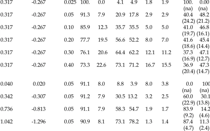
Table 3 repeats the analysis in Table 2 for the hedge fund sample. We use the Fung and Hsieh seven-factor model to compute alphas. The Appendix Table A.2 contains results using the Fama and French three-factor alphas for hedge funds. The
results are similar. Many of the patterns in Table 3 are similar to the results for the mutual funds. For example, in the first four rows of the table the BSW estimates of π0 decrease in (γ/2), and the power of the tests increases but remains substantially below 100% even at (γ/2) = 0.40. The empirical standard errors of the π fractions are larger for the hedge funds than we saw for the mutual funds, and they do not appear to increase with the size of the tests. (The reported standard errors, however, do increase with the test size, as can be seen in the Internet Appendix Table A.2.)
The hedge fund sample has a large spread of alpha estimates and especially t-ratios in the sample, as shown in Table 1. Because of this greater dispersion in the cross section, the power of the tests in Table 3 is generally lower than for the mutual fund sample -- never as high as 80%. Thus, the appeal of our approach, which allows for less than 100% power, is especially strong in the hedge fund sample. Table 3 also shows that the assumption in BSW that δ = 0 can be a poor approximation at larger test sizes. The table shows values in excess of 15% for some of the confusion parameters.
Our estimates of π0 in rows 6-9 of Table 3 range from 37-42%, substantially smaller than the BSW estimates, which are all near 91%. We find smaller fractions of zero alpha hedge funds and thus, more good and bad hedge funds. The fraction of funds to which we attribute zero alphas is greater when we assume that the true nonzero alphas are centered at more extreme values. When the alphas are “too large,” most of the funds will seem to have no ability. As we take the values of the good and bad fund alphas from further in the tails, the standard errors of the π fractions become smaller. When the data are generated from a mixture of distributions with more extreme alphas, it is easier to precisely determine to which subpopulation a nonzero
alpha fund belongs. The dependence of the inferences about the fractions on the choice of the true alpha parameters motivates our simultaneous estimation of the true alpha parameters and the π fractions, taken up in the next section.
Interestingly, our estimates of the fraction of good hedge funds is relatively stable for most of the different test sizes in Table 3, ranging from 36.9-41.6% across rows 2-6 of the table. (In the first row the estimates are not well-identified because the null and alternative hypotheses are so close.) There may be a substantial fraction of good hedge funds, unlike the evidence for mutual funds.
Panel B of Table 3 present the results when the true alpha parameters are set equal to the values that best fit the cross-section of the actual alpha estimates in the data. Results are shown for test sizes of 5% and 10%. In the first two rows we estimate that none of the hedge funds have zero alphas, whereas the BSW calculations would suggest 84.1-90.9%. We estimate that 51.7-53.2% of the hedge funds have positive alphas. The BSW calculations would suggest only 8.1-13.4%.
5.3. Fitting the Cross sectional Distribution
The previous tables show that inferences about the fractions of good and bad fund managers in the population are sensitive to the assumptions about the alphas of good and bad fund managers. Our estimates are more sensitive than the BSW
calculations. This is because the power of the tests is strongly sensitive to the true alpha parameters. The BSW calculations hold the power fixed at 1.0, but the actual power can be far below that, and our estimators reflect the variation in power across the parameter
values. The confusion parameters also vary with the alpha values, biasing π0 in the
opposite direction, but with a smaller effect.
In this section we search over the choice of the good and bad alpha parameters, and the corresponding estimates of the π fractions, to find those values of the
parameters that best fit the distribution of the t-ratios in the actual data, according to the Χ2 statistic in Equation (3). The best-fitting good and bad alpha parameters
minimize the difference between the cross section of fund alpha t-ratios estimated in the actual data, versus the cross section estimated from a mixture of return distributions, formed from the zero, good and bad alpha parameters and the estimated π fractions for each of the three types.
The good and bad alpha parameters, αg and αb, are found with a grid search. The search looks from the lower 5% to the upper 95% tail values of the alpha t-ratio estimates in the data, summarized in Table 1, with a grid size of 0.001% for mutual funds and 0.005% for hedge funds. At each point in the grid, the π fractions are estimated using simulation as in Tables 2 and 3. We start with models in which there are three groups, with zero, good and bad alphas as in BSW and the preceding analyses. In the first case, the search does not impose the restriction that the good alpha is
positive or the bad alpha is negative. The probability model remains valid without these restrictions, so we let the data speak to what are the best-fitting values.
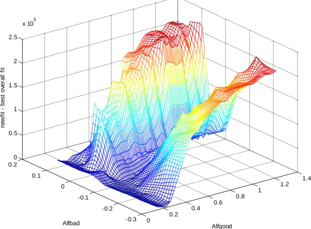
Figure 2 depicts an example of the results of the grid search for the true alpha parameters for hedge funds. The search is able to identify global optima at αg=0.237, αb = -0.098 for the hedge funds when the size of the tests is 5% in each tail. When the size is 10% the values are αg = 0.252, αb = -0.108, as shown in Panel B of Table 3. The Internet
Appendix (Table A.3) presents the joint estimation results using different values for the size of the tests, γ/2.12 At the best fitting alpha values, we estimate that none of the hedge funds have zero alphas, slightly more than 50% have the good alpha, and slightly under 50% have the bad, negative alpha. These figures are shown in Panel B of Table 3.
The joint estimation, as illustrated in Figure 2, reveals “valleys” in the criterion surface where linear combinations of the two nonzero alpha values produce a similar fit for the data. The impression is that three groups based on their alphas are plenty to describe the data, and that even fewer groups might suffice. Based on this impression we do not consider models with more than three groups.
The joint estimation for the three-group model applied to mutual funds finds two negative alphas and some zero alpha funds, but no funds with positive alphas. For the 5% and 10% test sizes, we estimate that 38.9% or 50.7% of mutual funds are “good” (which here, means zero alpha), 4.4% or 6.9% are “bad” (meaning, alphas of 0.087% or .034% per month) and the remaining 56.7 or 42.4% are “ugly” (meaning, alphas of -0.305% or -0.204% per month). The bad alpha estimates bracket the -0.267% per month value estimated by BSW, but our negative “good” alpha estimate is much smaller than the 0.317% value they estimate. These estimates are summarized in Panel B of Table 2.
The alpha values from our joint estimation are not as far out in the tails of the cross-section of alpha estimates from the actual data as are the values chosen by BSW. For example, values of αb are above the 25% left tail when the test size is 10%, and between the 25% and 10% tails when the size is 5%. Both values of αg are close to the
12 In their Appendix, BSW discuss choosing γ/2 in order to minimize an empirical mean squared error of the estimator for π0 around its minimum value, and Dewaele et al. (2011) also follow this approach.
median of fund alphas. The fact that the alpha values for the best fitting model are not far out in the tails means that in the best fitting model, the precision of the estimates will be lower than in a model with extreme alpha values, and the power of the tests will be lower, so that the assumption of 100% power in BSW will be a less accurate
approximation. The power parameters in Panel B of Table 2 are all below 60% for mutual funds. The power parameters in Panel B of Table 3 are all below 32% for hedge funds.
In the third and fourth rows of Panel B of Table 2, we summarize the results from repeating the joint estimation for mutual funds, where we constrain the values of the good alpha to be positive, and the bad alpha to be negative. The goodness-of-fit measures are larger, indicating a relatively poor fit to the data compared with the unconstrained case.13 It is interesting that the best-fitting good alphas for the mutual funds are very close to zero: 0.004% and 0.001% per month at the two test sizes. Because the good alphas are so close to zero, the zero-alpha null and the good-alpha alternative distributions are very close to each other. As a result, the power of the tests to find a good alpha and the confusion parameter δb are both very close to the size of the tests.
The evidence for mutual funds suggests that the best fitting alphas are either zero or negative, which motivates a simpler model with only two distributions in the population instead of three. The Internet Appendix describes the model when there are two distributions; one with alphas centered at zero and one with alphas centered at a
13 Asymptotically, the goodness-of-fit statistic is Chi-squared with 99 degrees of
freedom and the standard error is about 14. The p-values for all of the statistics and the differences across the models are essentially zero.
negative, value, αb. In the hedge fund sample, we let there be one zero and one positive alpha. The results are summarized in the third and fourth lines of Panels B of tables 2 and 3. For mutual funds the nonzero alpha is negative: -0.139% or -0.172% per month and the model says that 52-70% of the mutual funds have the negative alpha. For hedge funds the nonzero alpha is positive: 0.287% or 0.252% per month, and the estimates say that about 55% of the hedge funds have the positive alpha and 45% have a zero alpha. The larger fractions of zero alphas for hedge funds in the two-group model, compared to the three-group model makes sense, as the two-group model best fits the data by assigning a zero alpha to some of the previously negative alpha hedge funds. The goodness-of-fit shows that the two-group models do not fit the cross-section of funds’ alphas as well as the three-group models.
Finally, we consider models in which there is only a single value of alpha, around which all the mutual fund or hedge funds are centered. The results are summarized in the last two lines of Panels B of tables 2 and 3. For mutual funds, the single alpha is estimated to be negative, at -0.220% or -0.205% for the test sizes of 5% and 10%. For the hedge funds, the single alpha is estimated to be positive, at 0.452% or 0.434% for the test sizes of 5% and 10%. For mutual funds the goodness-of-fit statistics say that the one-group model fits the data better than the constrained three-group
model or the two-group model, but not as well as the unconstrained three-group model. For hedge funds the three-group model provides the best fit.
5.4 Rolling Estimation
We examine the models in rolling, 60 month estimation periods. Our goals are to see how stable the model parameters are over time and to detect any trends in the
parameters. In addition, we form portfolios of funds based on the estimated fractions in each subpopulation. If there is no information in the model’s parameter estimates about future performance, the subsequent return performance of the three groups should be the same. However, if the group of positive-alpha (negative-alpha) funds continues to have abnormal performance, it indicates persistence in the performance of the good (bad) funds.
Each 60-month estimation period produces parameter values that we interpret over time, and the end of each estimation period serves as a formation period for assigning each existing fund annually into one of the three groups. The first formation period ends in December of 1998 for hedge funds and in December of 1988 for mutual funds. The cross section during a formation period includes every fund with at least 8 observations (12 for hedge funds) during the formation period.14
Figures 3 and 4 summarize the time-series of estimates of the good and bad alphas for mutual funds and hedge funds, respectively. The bad alphas fluctuate with no obvious trend, but the good alphas show a marked downward trend for both mutual funds, and especially for the hedge funds. For the hedge funds the good alpha starts at more than 1% per month and leaves the sample at only 0.3%. The ending value is
14 BSW use five year fund performance records and a 60-month survival screen on the
funds. Fama and French (2010) criticize the 60 month survival screen, and we prefer not to impose such a stringent survival screen. If we encounter an alpha estimate larger than 100% per month in any simulation trial, we discard that simulation trial.
similar to the full sample estimate for the good alpha of 0.24% when the test size is 5%. For mutual funds, both the good and bad alphas are below zero after 2007, consistent with the full sample estimates. It makes sense that the full sample estimates are strongly influenced by the end of the sample, when there are many more funds in the data.
There are reasons to think that fund performance should be worse in more recent data. BSW (2010) find evidence of better performance in earlier subperiods of their sample. Cremers and Petajisto (2009) find a negative trend in funds’ active shares over time, and suggest that recent data may be influenced by more “closet indexing” among active mutual funds. Kim (2011) finds that the flow-performance relation in mutual funds attenuates after the year 2000, which could be related to a trend toward more similar performance in the universe of managers.
For both kinds of funds the good and the bad alphas get closer together over time. Figures 5 and 6 depict the time-series of the estimates of the fractions of good, bad and zero-alpha funds. We saw in Tables 2 and 3 that when the spread between the good and bad alphas is larger, as at the beginning of the rolling estimation period, the estimate of the π0 parameter is larger. We see this pattern in the figures. For mutual funds the π0 parameter starts the sample at large values and gets smaller over time. Our full sample estimate of 0.389 is close to the results for 2007-2010 near the end of the rolling sample. The fraction of bad funds, in contrast, rises until about 2007 and then declines at the end of the sample when the good alpha goes negative. For hedge funds, the πg parameter stays positive, and above 50% for most of the rolling sample, whereas the fraction of zero alpha funds stays at zero for the entire period.
Funds are sorted each year from low to high on the basis of their formation period alphas, and they are assigned to one of the three groups according to the current estimates of the π fractions. Equally-weighted portfolios of the selected funds are examined during a holding period. If a fund ceases to exist during a holding period, the portfolio allocates its investment equally among the remaining funds. The holding period is a one-year future period: Either the first, second, third or fourth year after formation. Thus, we examine how long-lived is the information, if any, in the past performance of the best or worst funds selected. The 60-month formation period is rolled forward year by year. This gives us a series of holding period returns for each of the first four years after formation, starting in January of 1999 for the hedge funds and in January of 1989 for the mutual funds. The holding period returns for the fourth year after formation start in January of 2002 for the hedge funds, and in January of 1992 for the mutual funds.
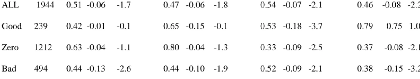
The average returns and their alphas during the holding periods are shown in Table 4. The alphas use the Fama and French factor model in the case of mutual funds, and the Fung and Hsieh factor model in the case of hedge funds. We show results for an equally-weighted portfolio of the selected good funds (Good), the funds in the zero-alpha group (Zero) and the funds in the bad zero-alpha group (Bad). For comparison
purposes, the first row (All) tracks an equally weighted portfolio of all the funds. Panel C presents results using the two-distribution model for mutual funds, where there are only zero alpha funds and bad funds.
The second columns of Table 4 show the averages of the numbers of funds in the various groups, averaged over the formation years. Consistent with Figure 6, most of
the hedge funds stay in the good alpha group. On average, 171 of 1386 hedge funds are in the bad group, and virtually none are in the zero alpha group. A portfolio of all hedge funds has a positive alpha over the holding periods, as do the good and bad-alpha groups. While membership in the good or zero-bad-alpha group produces t-ratio differences in the right direction, the differences are small, suggesting little predictive power for performance after formation.
For the mutual funds in Panel B and C of Table 4, there are more bad funds -- more than 400 on average in both the three- and the two-group models. The t-ratios of the holding period alphas generally line up as expected with the formation groups, suggesting that there may be some investment information in the groupings, but the differences are small. A similar result is found in Panel C, where the two-group model is summarized.
In the Internet Appendix, we present a variation on the rolling analysis, where we refine the false discovery methods used in BSW to group the funds into good and bad-alpha subsets, and follow the performance of the groups after the formation periods. The results using this approach are broadly similar to those in Table 4.
6. Simulating the Estimation by Simulation
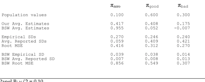
This section summarizes simulation exercises to evaluate small sample biases in the estimators and their standard errors. We use bootstrap simulations, drawing samples of the same sizes as in our actual data. In each of 1000 draws, artificial data are
generated from a mixture of three fund distributions, determined by given values of the π fractions and alphas. A given draw is generated by resampling months at random
from the hedge fund data, where the relevant fractions of the funds have the associated alphas added to each of their returns, after the sample estimates of their alphas have been subtracted. We use the hedge fund data because, as Table 1 suggests, the departures from normality are likely to be greater for hedge funds than for mutual funds, providing a tougher test of the finite sample performance. Initially, the values of the π fractions are set to π0=0.10, πg=0.60 and πb=0.30, and the bad and good alphas are set
to -0.138 and +0.262% per month.15
For each draw of artificial data from the mixture with known parameters, we run the estimation by simulation, for a fixed value of the size of the tests, γ/2. The π
fractions are estimated in each of these trials from the three simulations as described earlier in the paper, each using 1000 artificial samples generated by resampling from the one draw from the mixture distribution, treating that draw the same way we treat the original sample. The α parameters are held fixed for these simulations. The Avg. estimates in Table 5 are the averages over the 1000 draws from the mixture distribution. The empirical SD’s are the standard deviations taken across the 1000 draws. The Root MSE’s are the square roots of the averages over the 1000 draws, of the squared
difference between an estimated and true parameter value.16
15 We experiment with setting all the π fractions to 1/3 and the results, shown in the Internet Appendix, are broadly similar. We also report experiments where we set the π fractions to the banner values reported by BSW: π0=0.75, πg=0.01 and πb=0.24, and find broadly similar results.
16 In the event that a parameter estimate is on the boundary of the parameter space (a π fraction is zero or 1.0), we drop the estimated standard error for that simulation trial for the calculations. This choice has only a small effect on the results.
Consistent with our analytical results, Table 5 shows that the BSW estimator of π0 is badly biased in favor of finding too many zero-alpha funds, and the estimators of the fractions of good and bad funds are biased toward zero. When 10% of the funds have zero alphas, the BSW estimates are 75-96%, depending on the size of the tests. The negative point estimate of πbwhich we observed in the sample is consistent with the
negative average value in the simulations, for the 5% and 10% test sizes. Our point estimates are also biased. Like the BSW estimates we find too many zero alpha funds and too few good and bad funds. But our point estimates are much less biased than the BSW estimators, finding for example, 20-42% zero alpha funds when the true fraction is 10%.
Our point estimates are typically within one empirical standard deviation of the true values of the π fractions at the 5% test size, while the BSW estimators are much further away. Our estimator is more accurate at the 10% size and slightly more accurate still at the 20% size, where the expected point estimate is within 0.3-0.6 standard errors of the true parameter value. Consistent with the analytical results, the BSW estimates are less biased at the larger test sizes, but they are still are badly biased. The point estimates remain more than six empirical standard errors away from the true values when the test size is 20%.
Our results indicate that smaller fractions of funds have zero alphas and larger fractions have nonzero alphas, compared with the evidence using the BSW
methodology. We also find that large fractions of the hedge funds are estimated to have either positive or negative alphas. The finite sample performance of the estimators
says that these claims are likely conservative. Given the biases in the estimators, the fractions of zero alpha funds are likely even smaller than we report above.
The BSW reported standard errors understate the sampling variability of their estimates for all test sizes. Even when γ/2=0.20 or 0.30 (Panels C and D), where they perform the best, the average BSW standard errors range from 20% to 60% of the
empirical standard errors.17 Our standard error estimates are also biased. When the test size is 5% they are too far small for π0 and too large for πg and πb by as much as a factor of two. When the size is 10% the standard errors are reasonably accurate for π0 but still too large for πg and πb by 50-100%.18
The empirical standard errors in Table 5 get smaller as the size of the tests is increased from 5% to 20%. The average empirical standard error at the 20% size is about 60% of the value at the 5% size. This is the opposite of the pattern in the average reported standard errors, which are larger at the larger test sizes. Given this tradeoff, the 10% test size appears to be the best choice if relying on reported standard errors. The point estimates are as accurate as at the larger test sizes. The reported standard errors for π0 are fairly accurate, and they are overstated for πg and πb, and thus conservative.
Finally, the simulations show that the BSW estimators display lower sampling variability than our estimators. This makes sense, given the relative simplicity of their estimators that results from setting the power to 100% and the confusion to zero.
17As a check, the reported standard error in BSW (Table II) for πb is 2.3%. Our simulations of the reported BSW standard errors, when γ/2=0.20, average 2.2%, suggesting that we are accurately representing their standard error calculations.
18We conduct some experiments where we set the correlation of the tests across funds to zero, as assumed by BSW, and we find that the standard errors are then an order of magnitude too small.
However, the BSW estimators concentrate around biased values. Comparing the root mean squared errors (RMSEs), they are substantially higher for the BSW estimators. When the test size is 5%, the RMSE of the BSW estimator is larger than for our estimator by 100-200%. As the test size is increased the RMSEs of both estimators is smaller, but the BSW estimator still has a larger RMSE. When the size is 20%, the BSW estimators RMSEs are larger than for our estimators by 150-300%.
Panel D of Table 5 takes the size of the tests to 30% in each tail. The average point estimates, RMSEs and empirical standard errors of our estimators are similar to those in Panel C, but the average reported standard errors are more overstated. The BSW point estimates have similar biases, and the BSW reported standard errors still average only 30-60% of the empirical standard errors. The RMSEs are slightly improved, but still larger than the RMSEs of our estimators, by 160-300%.
We conduct some experiments where we expand the number of time-series observations in the simulations to 5,000, in order to see which of the biases are finite sample issues, and which are inconsistencies. (These experiments are reported in the Internet Appendix.) The large-sample experiments suggest that the BSW standard error estimators are consistent. The experiments also suggest that the BSW point estimator of π0 is inconsistent. For example, the average estimated value is about 30% when the true value is 10%, and the expected estimate is 49% when the true value is 1/3. Our
estimates are much closer to the true values when T=5,000, suggesting that their biases in Table 5 are likely finite sample biases.
7. Robustness
This section describes a number of experiments to assess the sensitivity of our results to several issues. These include a possible relation between funds’ alphas and active management, the level of noise in the simulated fund returns, alternative factor models and return smoothing.
7.1. Are the Simulated Returns too Noisy?
Kowsowski et al. (2006) find that the best performing funds have significant positive alphas, but Fama and French (2010) do not find significant performance. One of the differences between the studies is the method of simulating fund returns. Fama and French and the preceding tables resample, under the null hypothesis that the true alphas are zero, from the vector of factors and the actual fund returns minus their estimated alphas. Kowsowski et al. resample from the factor model residuals. Fama and French argue that this approach understates the sampling error by ignoring the sampling variation in the factors. However, the more conservative approach suggested by Fama and French does not account for the fact that the alphas have been estimated with error, because in each simulation trial and for each fund the estimated alphas are treated as constants. In the cross-section, the alphas are random variables subject to estimation error. We conduct an experiment which accounts for the fact that the
estimated alphas contain measurement error. We adjust the simulations to account for estimation error in the alphas.
Instead of subtracting the estimated alpha from a fund in the simulations as if it was constant, we subtract a normally distributed random variable, with mean equal to the point estimate of alpha and standard deviation equal to the heteroskedasticity-consistent standard error of the alpha estimate. The results of this experiment are summarized in the Internet Appendix, Table A.3, Panel E.
good alpha estimate is larger by about 0.05% per month and the bad alpha estimate is smaller by a similar amount. The power and confusion parameters are similar. The fraction of zero-alpha hedge funds is now estimated to be larger than zero, at 0.02% to 12.4% depending on the test size, but remains within one standard deviation of zero. The BSW estimates are similar to the previous results.
7.2 Are the Alphas Correlated with Active Management?
Studies suggest that more active funds have larger alphas (e.g. Cremers and Petajisto (2009), Titman and Tiu (2011), Amihud and Goyenko (2013) and Ferson and Mo (2015)). In particular, funds with lower market model regression R-squares are found to have larger alphas. We examine the correlations between the factor model R-squares and the estimated alphas and find a correlation of -0.015 in the mutual fund sample and -0.111 in the hedge fund sample. The mixtures of distributions simulated above do not accommodate this relation.
We modify the simulations to allow a relation in the cross-section of funds’ returns, between alpha and a fund’s active management measured by the R-squares in the factor model regressions that deliver the alphas. We sort the funds in the original data by their factor model R-squares, group them into three groups with the group sizes determined by the -fractions at any point in the simulations, and assign the good alpha first to the low R-square group and the bad alpha first to the high R-square group. The simulations draw the vector of factors and fund returns, so they preserve the relation between the random part of fund returns and the factors. Thus, this approach builds in a relation between the alpha and active management, measured by the factor model R-squares.
The results from this variation on the simulations are summarized in the Internet appendix, Table A.3, Panel D. We find that this modification also improves the
funds are similar to those in the original design, but the estimate of the bad alpha is smaller, at -0.35% to -0.37%, while in the original design it was about -0.1% per month. Fewer fractions of the hedge funds are estimated to have this more pessimistic bad alpha, and as a result the fraction of zero alpha hedge funds is increased to 30%-44%, which is a significant positive fraction when the test size is 10%. The BSW estimates are similar to those in the original design.
This experiment illustrates that when the probability model incorporates an association between the hedge funds’ alphas and the cross-section of the regression R-squares, the best-fitting alpha parameters are further out in the tails, and in particular in the left tail, where it moves about ¼ of a percent to the left. This suggests that the
relatively poor performance of the high R-square hedge funds is the dominant part of the relation between the R-squares and performance. This result may not be surprising, but it does suggest that future work on estimation by simulation might profit from building in associations between other fund characteristics and the performance groups.
7.3 Alternative Alphas
While the Fama and French (1996) three-factor model is less controversial for fund performance evaluation than for asset pricing, it is still worth asking if the results are sensitive to the use of different models for alpha. We examine two alternatives for mutual funds: one with fewer factors and one with more factors. The first is the Capital Asset Pricing Model (Sharpe, 1964), with a single market factor and the second is the Carhart (1997) model, which adds a momentum factor. For the hedge fund sample we use the multifactor model of Fung and Hsieh (2001, 2004) in the main tables and try the Fama and French three factor model as a robustness check. Results using the