“You Might Also Like:”
Privacy Risks of Collaborative Filtering
Joseph A. Calandrino
1, Ann Kilzer
2, Arvind Narayanan
3, Edward W. Felten
1, and Vitaly Shmatikov
2 1Dept. of Computer Science, Princeton University
{jcalandr,felten}@cs.princeton.edu 2Dept. of Computer Science, The University of Texas at Austin
{akilzer,shmat}@cs.utexas.edu3
Dept. of Computer Science, Stanford University
Abstract—Many commercial websites use recommender sys-tems to help customers locate products and content. Modern recommenders are based on collaborative filtering: they use patterns learned from users’ behavior to make recommendations, usually in the form of related-items lists. The scale and complexity of these systems, along with the fact that their outputs reveal only relationships between items (as opposed to information about users), may suggest that they pose no meaningful privacy risk.
In this paper, we develop algorithms which take a moderate amount of auxiliary information about a customer and infer this customer’s transactions from temporal changes in the public outputs of a recommender system. Our inference attacks are passive and can be carried out by any Internet user. We evaluate their feasibility using public data from popular websites Hunch, Last.fm, LibraryThing, and Amazon.
I. INTRODUCTION
Recommender systems are ubiquitous on the Web. When you buy products from Amazon, rent movies on Netflix, listen to music on Last.fm, or perform myriad other tasks online, recommender systems make suggestions based on your behavior. They typically rely on collaborative filtering, or patterns learned from other users: for example, “customers who buy item X (as you just did) often buy item Y.”
We investigate the privacy risks of recommender systems based on collaborative filtering. By design, such systems do not directly reveal behavior of individual users or any “personally identifiable information.” Their recommendations are based on aggregated data involving thousands to millions of users, each with dozens to thousands of transactions. More-over, modern collaborative filtering leverages relationships between items rather than relationships between users, creating an extra level of indirection between public recommendations and individual transactions. One might therefore assume that it is infeasible to draw meaningful inferences about transactions of specific users from the public outputs of recommender systems. We show that this assumption is wrong.
Our contributions. We develop a set of practical algorithms that allow accurate inference of (partial) individual behavior from the aggregate outputs of a typical recommender system. We focus on item-to-item collaborative filtering, in which the system recommends items similar to a given item. Our key insight is to exploit the dynamics of public recommendations
in order to make the leap from aggregate to individual data. This paper is the first to make and quantitatively evaluate the
observation that temporal changes in aggregate recommenda-tions enable accurate inference of individual inputs.
Our algorithms require only passive, “black-box” access to the public outputs of a recommender system, as available to any Internet user. The attacker need not create fake customers or enter purchases or ratings into the system. We do not assume that customers’ transactions are available in either identifiable or anonymized form. Our approach is thus fundamentally different from the techniques for re-identifying anonymized transactional records [26]. Re-identification assumes that the attacker has direct access to customers’ records. By contrast, our attacks rely only on indirect access: the records are fed into a complex collaborative filtering algorithm and the attacker’s view is limited to the resulting outputs.
Our algorithms monitor changes in the public outputs of rec-ommender systems—item similarity lists or cross-item correla-tions—over a period of time. This dynamic information is then combined with a moderate amount of auxiliary information
about some of the transactions of a particular “target” user. The combination is used to infer many of the target user’s unknown transactions with high accuracy. Auxiliary information can be obtained by analyzing the user’s publicly revealed behavior; we discuss this in more detail in Section III.
Overview of results.We evaluate our algorithms on real-world recommender systems which produce different types of rec-ommendations. Our goal is not to claim privacy flaws in these specific sites—in fact, we often use data voluntarily disclosed by their users to verify our inferences—but to demonstrate the general feasibility of inferring individual transactions from the outputs of collaborative filtering systems.
Some recommender systems make item-to-item correlations available. An example is Hunch, a popular recommendation and personalization website. There is a tradeoff between the number of inferences and their accuracy. When optimized for accuracy, our algorithm infers a third of the test users’ secret answers to Hunch questions with no error.
Other recommender systems make only item similarity or “related items” lists available, with or without numeric similar-ity scores. Examples include Last.fm, an online music service, and LibraryThing, an online book cataloging service and recommendation engine. The results from our LibraryThing experiment illustrate the yield-accuracy tradeoff, ranging from
58 inferences per user with 50% accuracy to 6 inferences per user with 90% accuracy. Another example of item similarity lists is the “Customers who bought this item also bought . . . ” feature on Amazon. Our ability to evaluate our algorithms on Amazon’s recommender system is constrained by the lack of a “ground-truth oracle” for verifying our inferences, but we conducted a limited experiment to demonstrate the feasibility of adversarial inference against Amazon’s recommendations.
By necessity, our experiments on real-world systems involve only a limited sample of users. To demonstrate that our inference algorithms also work at scale, we implemented an item-to-item collaborative filtering engine very similar to that used by Amazon, and ran it on the Netflix Prize dataset of movie-rating histories [28]. This allowed us to simulate a complete system, producing public recommendations as well as auxiliary information about users. The underlying dataset of individual ratings served as the “ground-truth oracle” for verifying inferences made by our algorithm. Our algorithm was able to infer 4.5% of transactions of sufficiently active users with an accuracy of90%.
There is a passing similarity between our inference algo-rithms and actual collaborative filtering. Both use statistical methods to reach probabilistic conclusions about unknown aspects of users’ behavior. Our algorithms, however, are tech-nically different and pursue a fundamentally different goal: not to predict future events, but to infer past events. This translates into several concrete differences, discussed in Section V. For example, in contrast to prediction algorithms, ours perform best when a user deviates from normal patterns and if his transactions involve less popular items. We can also infer an approximate date when a transaction occurred.
For completeness with respect to different types of recom-mender systems, we present a simple active attack on user-based collaborative filtering. In broad terms, the attacker cre-ates multiple sybil users whose transactional profile is similar to what he knows about the target user’s profile and infers the target’s non-public transactions from the recommendations made by the system to these sybils.
In summary, this work is the first to develop a generic method for inferring information about individual users’ trans-actions from the aggregate outputs of collaborative filtering. We show that public outputs of common recommender al-gorithms may expose non-public details of individual users’ behavior—products they purchase, news stories and books they read, music they listen to, videos they watch, and other choices they make—without their knowledge or consent.
II. SURVEY OF RECOMMENDER SYSTEMS
Recommender systems have become a vital tool for attract-ing and keepattract-ing users on commercial websites. Their utility is supported by research [14] as well as common practice.
The task of a recommender system can be abstractly de-scribed as follows. Consider a matrix in which rows corre-spond to users and columns correcorre-spond to items. Each value in this matrix represents a user’s revealed or stated preference (if any) for an item: for example, whether he purchased a book,
how many times he listened to a song, or what rating he gave to a movie. Because the item set is typically far larger than a single user can consume and evaluate, this matrix is “sparse:” only a small fraction of entries are filled in. A recommender system takes this matrix as input, along with any available metadata about users (such as demographics) and items (such as item categories). The goal of the system is to extrapolate users’ “true” preferences over the full item set.
Recommender systems can provide several types of rec-ommendations. If the system suggests items to an individual user based on its knowledge of the user’s behavior, it provides
user-to-itemrecommendations. If the system helps users find similar users, it provides user-to-user recommendations. If, given an item, the system suggests similar items, it provides
item-to-itemrecommendations. The system may even list users who are strongly associated with a given item, thus providing
item-to-userrecommendations. The same system may provide several types of recommendations: for example, Last.fm pro-vides both item-to-item and user-to-user recommendations.
We focus on item-to-item recommendations, both because they are supported by essentially all popular online recom-mender systems and because their output is typically public and thus the most feasible avenue for an attack.
A thorough technical survey of the literature on recom-mender systems can be found in [1]. Recomrecom-mender systems can be classified as content-based, collaborative, and hybrid. Content-based systems identify relationships between items based on metadata alone and recommend items which are similar to the user’s past transactions. Purely content-based recommender systems pose no privacy risks under our attacks, since the system does not consider other users’ transactions when making recommendations to a user.
Collaborative filtering is much more robust and domain-agnostic, and hence far more popular. Collaborative filtering identifies relationships between items based on the preferences of all users. Traditional collaborative filtering methods are
user-based. For a given user, the system finds other users with a similar transaction history. In the user-to-user case, the system recommends these similar users; in the user-to-item case, it recommends items selected by the similar users.
The alternative is item-based collaborative filtering, which was first described by Sarwar et al. [31] and has become the dominant approach [2, 20, 21]. It generates recommendations usingitem similarity scoresfor pairs of items, which are based on the likelihood of the pair being purchased by the same customer. Although some systems make raw similarity scores public, their main uses are internal: for example, to find items which are similar to a user’s previously purchased items in order to make user-to-item recommendations.
A. Item-to-item recommendations
It has become standard practice for online recommender systems to publish item-to-item recommendations, usually in the form ofitem similarity listsproduced from item similarity scores. Given an item, these lists help find related items (see [6] for a survey of algorithms). On Amazon, this is seen as
the “Customers who bought this item also bought . . . ” feature. Similar features are found on many commercial websites, including iTunes, Last.fm, Pandora, Netflix, YouTube, Hulu, and Google Reader. Item similarity lists even appear on many sites that do not have traditional user-to-item recommenda-tions, such as IMDb, CNN, and the New York Times.1 Item
similarity lists may be limited to top N items or contain an ordered list of hundreds or thousands of items.
Many systems reveal additional information. Amazon re-veals not only the relative popularity of items via bestseller lists and “sales rank,” but also the percentage of users pur-chasing certain other items after viewing the given item.2For every song, Last.fm provides the number of listeners and how many times it was played by each listener. Given a book, LibraryThing provides several ordered lists of related books, including more common and more obscure recommendations; some lists also contain detailed transaction information, such as the precise number of users who have both books. Finally, Hunch gives all users access to the entire item-to-item co-variance matrix via an API.
B. User-to-item recommendations
User-to-item recommendations may be user-based (finding similar users and recommending their items) or item-based (finding items related to ones that the user chose in the past). Amazon provides several personalized lists with up to 1,000 items to logged-in users. LibraryThing, Last.fm, and Netflix also provide recommendation lists to their users.
III. ATTACK MODEL
We view the data that the system uses to make recommenda-tions as a matrix where rows correspond to users and columns to items. Each cell represents a transaction (e.g., the user’s purchase or stated preference for an item). Entries may be dated; the date may or may not be sensitive from a privacy perspective. As users interact with the system, the matrix is continually updated and new recommendations are generated. Our primary focus is on passive inference attacks. The attacker has access to the public outputs of the recommender system, which, depending on the system, may include item similarity lists, item-to-item covariances, and/or relative pop-ularity of items (see Section II). The outputs available to the attacker are available to any user of the system. Crucially, the attacker observes the system over a certain period and can thus capture changesin its outputs: an increase in covariance between certain items, appearance of an item on the similarity list of another item, an increase in an item’s sales rank, etc.
Note, however, that each update incorporates the effects of hundreds or thousands of transactions. With the exception of auxiliary information (described below), inputs into our inference algorithms are based on aggregate statistics and con-tain neither personally identifiable information nor information about specific transactions.
1Even offline retailers such as supermarkets frequently deploy item-to-item similarity analysis to optimize store layout [3].
2We do not exploit the latter information for the inference attacks in this paper. This is an interesting topic for future research.
For completeness, we also briefly consider active attacks, where the attacker creates fake, “sybil” users and manipulates their entries in the corresponding rows of the transaction matrix. Depending on the system, this includes adding new entries (easy in the case of ratings and stated preferences, more expensive for purchases), modifying existing entries, or deleting them (easy in the case of ratings and preferences and may also be possible for purchases; for example, one can instruct Amazon to ignore certain purchases when making recommendations). Observable outputs include items recom-mended by the system to the sybil users and, in the case of systems like Last.fm or LibraryThing, also user similarity lists which explicitly identify users with similar histories.
Auxiliary information. We assume that for some users, a subset of their transaction history is available to the attacker. We refer to this as the attacker’s auxiliary information. An inference attack is successful if it enables the attacker to learn transactions which are not part of the auxiliary information. In other words, the attacker’s objective is to “leverage” his prior knowledge of some of the target user’s transactions to discover transactions that he did not know about.
There are many sources of auxiliary information. The first is the target system itself. On many websites, users publicly rate or comment on items, revealing a high likelihood of having purchased them. The system may even publicly confirm the purchase,e.g., “verified purchase” on Amazon. Alternatively, on sites with granular privacy controls, some of the transac-tions may be publicly visible, while others remain private.
The second source is users revealing partial information about themselves via third-party sites. This is increasingly common: for example, music websites allow embedding of tracks or playlists on blogs or other sites, while Amazon Kindle allows “tweeting” a selected block of text; the identity of the book is automatically shared via the tweet.3
The third source is data from other sites which are not directly tied to the user’s transactions on the target site, but leak partial information about them. For example, books listed in a Facebook user profile reveal partial information about purchases on Amazon. Linking users across different sites is a well-studied problem [17, 27]. On blippy.com, “a website where people obsessively review everything they buy,” individual purchase histories can be looked up by username, making linkages to other sites trivial. Note that the third (and to a lesser extent, the second) source of auxiliary information is outside the control of the recommender system.
Furthermore, information about users’ behavior is con-stantly leaked through public mentions on online fora, real-world interactions with friends, coworkers, and acquaintances,
etc.Therefore, we do not consider the availability of auxiliary information to be a significant impediment to our attacks.
3The stream of such tweets can be conveniently accessed in real time by searching Twitter for “amzn.com/k/”.
Algorithm 1: RELATEDITEMSLISTINFERENCE
Input: Set of target itemsT, set of auxiliary itemsA, scoring function :R|A|→R
Output: Subset of items fromT which are believed by the attacker to have been added to the user’s record inf erredItems={}
foreachobservation timeτ do
∆= observation period beginning atτ
N∆=delta matrix containing changes in positions of items fromT in lists associated with items fromA foreachtarget itemtinN∆ do
scorest=SCOREFUNCTION(N∆[t]) ifscorest≥thresholdandt /∈ Athen
inf erredItems=inf erredItems∪ {t} returninf erredItems
IV. GENERIC INFERENCE ATTACKS
A. Inference attack on related-items lists
In this setting of the problem, the recommender system outputs, for each item, one or more lists of related items. For example, for each book, LibraryThing publishes a list of popular related books and a list of obscure related books.
The description of the inference algorithm in this section is deliberately simplified with many details omitted for clarity. Intuitively, the attacker monitors the similarity list(s) associ-ated with each auxiliary item (i.e., item that he knows to be associated with the target user). The attacker looks for items which either appear in the list or move up, indicating increased “similarity” with the auxiliary item. If the same target item t appears and/or moves up in the related-items lists of a sufficiently large subset of the auxiliary items, the attacker infers thatt has been added to the target user’s record.
Algorithm 1 shows the inference procedure. Intuitively, delta matrices N∆ store information about the movement of each
target item t in the related-items lists of auxiliary items A
(we defer the discussion of matrix construction). The attacker computes a score for each t using a scoring function. The simplest scoring function counts the number of auxiliary items in whose related-items liststhas appeared or risen. If the final score exceeds a predefined threshold, the attacker concludes that t has been added to the user’s record.
Scoring can be significantly more complex, taking into account full dynamics of item movement on related-items lists or giving greater weight to certain lists. To reduce false positives and improve inference accuracy, the scoring function must be fine-tuned for each system. For example, recommender systems tend to naturally cluster items. Netflix users who watched the DVD of the first season of “The Office” also tend to watch the second season. Suppose that some movie rises in the similarity lists of both seasons’ DVDs. Because the overlap in viewers across seasons is so great, this does not reveal much more information than a movie rising in the list associated with a single DVD. In fact, it may reveallessif users who watch only one of the two seasons are very unusual. Our scoring functions prefer sets of auxiliary items which span genres or contain obscure items. Consider LibraryThing,
where users share the books they read. Classics such as To Kill a MockingbirdorCatcher in the Ryeare so common that changes in their similarity lists tend to result from widespread trends, not actions of a single user. Movement of a book in a list associated with an obscure book reveals more than movement in a list associated with a bestseller.
B. Inference attack on the covariance matrix
In this setting of the problem, the item-to-item covariance matrix is visible to any user of the system. An example of an online recommender system that reveals the covariance matrix is Hunch (see Section VI-A). We also explain complications, such as asynchronous updates to the system’s public outputs, which apply to the related-items scenario as well.
LetI be the set of items. The recommender system main-tains an item-to-item matrix M. For any two distinct items i, j ∈ I, the (i, j) cell of M contains a measure of the similarity betweeniandj. In the setting of this section,(i, j) and(j, i)contain the covariance betweeniandj. In the setting of Section IV-A, the(i, j)cell contains the position, if any, of itemi inj’s related-items list, along with additional informa-tion such as numeric similarity strength. As users interact with the recommender system by making purchases, entering their preferences, etc., the system continually accumulates more data and updatesM at discrete intervals.
For each user u, the recommender system maintains a “record”Su⊂ I. As the user interacts with the system, some
itemtmay be added toSu, reflecting thattis now related to
the user. In some systems, the same item may be added toSu
multiple times: for example, the user may listen to a particular song, watch a movie, or purchase a product more than once. The system may also remove items fromSu, but this is less
common and not used for our attack.
Consider a toy case when a single useruinteracts with the system between time τ1 andτ2 =τ1+ ∆, and t is added to
the user’s item list Su. Covariance between t and all other
items inSu must increase. LetM1 be the matrix at time τ1, M2 the matrix at time τ2, and M∆ =M2−M1. Then, for
all itemssi∈ Su, the(si, t)entry ofM∆ will be positive. Of
course, real-world recommender systems interact concurrently with multiple users whose item sets may overlap.
Intuitively, the attack works as follows. The attacker has auxiliary information about some items in the target user’s record (Section III). By observing simultaneous increases in covariances between auxiliary items and some other itemt, the attacker can infer thatt has been added to the user’s record.
Formally, the attacker’s auxiliary information is a subset
A ⊆ Su. It helps—but is not necessary—if A is uniquely
identifying, i.e., for any other user uj of the recommender
system, A * Suj. This is possible if items in A are less
popular or ifAis large enough [26].
The attacker monitors the recommender system and obtains the covariance matrixM at each update. LetT ⊆ I \Abe the set of items the user may have selected. The attacker observes the submatrix ofM formed by rows corresponding to the items inT ∪ A and columns corresponding to the items inA. Call
this submatrix N. Since A ⊆ Su, when an item t ∈ T is
added to Su, covariances between t and many ai ∈ A will
increase. If the attacker can accurately recognize this event, he can infer that thas been added to Su.
The inference procedure is significantly complicated by the fact that when an item is added toSu, not all of its covariances
are updated at the same time due to processing delays. In particular, (t, ai) covariances for ai ∈ A may update at
different times for different auxiliary items ai. Furthermore,
auxiliary items may enter the system at or around the same time as t. We cannot use the (t, ai)covariance unless we are
certain that the addition of item ai to u’s record has been
reflected in the system. Before attempting an inference, we compute the subset of auxiliary items which “propagated” into the covariance matrix. The algorithm works by measuring increases in pairwise covariances between auxiliary items; we omit the details due to space limitations. In the following, we refer to this algorithm as PROPAGATEDAUX.
Constructing delta matrices. Suppose the attacker observes the covariance submatrices Nτ1, Nτ2, . . . at times τ1, τ2, . . ..
For each observation, the attacker creates a delta matrix N∆
which captures the relevantchangesin covariances. There are several ways to build this matrix. In the following, τmax is a
parameter of the algorithm, representing the upper bound on the length of inference windows.
Strict time interval.For eachτi, setN∆=Nτi+1−Nτi. Since
not all covariances may update between τi and τi+1, some
entries inN∆ may be equal to 0.
First change.For eachτi,N∆ consists of the first changes in
covariance after τi. Formally, for each entry(x, y) of N, let
τk > τi be the first time after τi such that τk ≤ τmax and Nτk[x][y]6=Nτi[x][y]. SetN∆[x][y] =Nτk[x][y]−Nτi[x][y].
Largest change. Similar to first change.
Making an inference. The attacker monitors changes in the submatrix N. For each relevant interval ∆, the attacker computes the delta matrix N∆ as described above and uses
PROPAGATEDAUX to compute which auxiliary items have propagated into N. Then he applies Algorithm 2. In this algorithm, scoreSett is the set of all auxiliary items whose
pairwise covariances with t increased, supportt is the
sub-set of scoreSett consisting of auxiliary items which have
propagated, scoretis the fraction of propagated items whose
covariances increased. Ifscoret andsupportt exceed certain
thresholds (provided as parameters of the algorithm), the attacker concludes thatt has been added to the user’s record. Inference algorithms against real-world recommender sys-tems require fine-tuning and adjustment. Algorithm 2 is only a high-level blueprint; there are many system-specific variations. For example, the algorithm may look only for increases in covariance that exceed a certain threshold.
C. Inference attack on kNN recommender systems
Our primary focus is on passive attacks, but for complete-ness we also describe a simple, yet effective active attack on
Algorithm 2: MATRIXINFERENCE
Input: Set of target itemsT, set of auxiliary itemsA, PROPAGATEDAUX returns a subset ofA, implementation-specific parameters thresholdsupport,score
Output: Subset of items fromT which are believed by the attacker to have been added toSu
inf erredItems={} foreachobservation timeτ do
propagatedτ =PROPAGATEDAUX(A, τ) ∆= observation period beginning atτ
N∆=delta matrix containing changes in covariances between items inT ∪ A
foreachitemtin T do
scoreSett=subset ofa∈ Asuch thatN∆[t][a]>0
supportt=|scoreSett∩propagatedτ| scoret=|propagated|supportt|
τ|
ifscoret≥thresholdscoreand supportt≥thresholdsupportthen
inf erredItems=inf erredItems∪ {t} returninf erredItems
thek-nearest neighbor (kNN) recommendation algorithm [1]. Consider the following user-to-item recommender system. For each userU, it finds thekmost similar users according to some similarity metric (e.g., the Pearson correlation coefficient or cosine similarity). Next, it ranks all items purchased or rated by one or more of these k users according to the number of times they have been purchased and recommends them to U in this order. We assume that the recommendation algorithm and its parameters are known to the attacker.
Now consider an attacker whose auxiliary information con-sists of the userU’s partial transaction history,i.e., he already knowsmitems that U has purchased or rated. His goal is to learnU’s transactions that he does not yet know about.
The attacker createsksybil users and populates each sybil’s history with the m items which he knows to be present in the target user U’s history. Due to the sparsity of a typical transaction dataset [26], m ≈ O(logN) is sufficient for the attack on an average user, where N is the number of users. (In practice, m ≈ 8 is sufficient for datasets with hundreds of thousands of users.) With high probability, the k nearest neighbors of each sybil will consist of the otherk−1 sybils and the target userU. The attacker inspects the list of items recommended by the system to any of the sybils. Any item which appears on the list and is not one of the m items from the sybils’ artificial history must be an item thatU has purchased. Any such item was not previously known to the attacker and learning about it constitutes a privacy breach.
This attack is even more powerful if the attacker can adaptively change the fake history of his sybils after observing the output of the recommender system. This capability is supported by popular systems—for example, Netflix users can change previously entered ratings, while Amazon users can tell the site to ignore certain transactions when making recommendations—and allows the attacker to target multiple users without having to create new sybils for each one.
D. Attack metrics
Our attacks produce inferences of this form: “Item Y was added to the record of user X during time period T.” The main metrics are yield and accuracy. Yield is the number of inferences per user per each observation period, regardless of whether those inferences are correct. Accuracy is the percentage of inferences which are correct. We use yield rather than alternative metrics that focus on the number of correct inferences because the attacker can adjust the parameters to control the number of inferences made by our algorithm but cannot directly control the number or proportion that are correct. Where it makes sense, we also express yield as the percentage of the user’s transactions inferred by our algorithm, but in general, we focus on the absolute number of inferences. High yield and high accuracy are not simultaneously nec-essary for an attack to be dangerous. A single accurate inference could be damaging, revealing anything from a medical condition to political affiliation. Similarly, a large number of less accurate inferences could be problematic if their implications are uniformly negative. While the victim may retain plausible deniability for each individual inference, this provides little or no protection against many privacy violations. For example, plausible deniability does not help in situations where judgments are based on risk (e.g., insurance) or prejudice (e.g., workplace discrimination), or where the inferred information further contributes to a negative narrative (e.g., confirms existing concerns that a spouse is cheating).
There is an inherent tradeoff between yield and accuracy. The higher the yield, the higher the number of incorrect infer-ences (“false positives”). Different combinations of parameters for our algorithms produce either more inferences at the cost of accuracy, or fewer, but more accurate inferences. Therefore, we evaluate our algorithms using the yield-accuracy curve.
V. INFERENCE VS.PREDICTION
At first glance, our inference algorithms may look similar to standard collaborative filtering algorithms which attempt to
predictthe items that a user may like or purchase in the future based on his and other users’ past transactions.
The two types of algorithms are completely different, both technically and conceptually. We infer the user’sactual trans-actions—as opposed to using the known behavior of similar users to guess what he may do or have done. Prediction algo-rithms discover common patterns and thus have low sensitivity to the presence or absence of a single user. Our algorithms are highly sensitive. They (1) work better if there are no similar users in the database, but (2) do not work if the target user is not the database, even if there are many similar users.
Collaborative filtering often exploits covariances between items; our algorithms exploitchangesin covariance over time. The accuracy of predictions produced by collaborative filtering does not change dramatically from period to observation period; by contrast, we infer the approximate datewhen the transaction occurred, which is very hard to discover using collaborative filtering. Finally, our algorithms can infer even transactions involving very obscure items. Such items tend to
populate lower ranges of auxiliary items’ similarity lists, where a single transaction has the biggest impact. Section VII shows that transactions involving obscure items are more likely to be inferred by our algorithms.
Prediction quality can be seen as a baseline for feasible inference quality. A prediction is effectively an expected probability that a user with item a will select some target itemt at any time. If a user with itemaselects itemt during a given time period, he exceeds this expected probability, causing a temporary rise (until other users balance the impact). By looking at changes in predictions over short periods of time, we can reconstruct how user behavior deviated from the predictions to produce the observed changes. This yields more accurate information than predictions alone. As Sections VI-A and VII show, our algorithms not only outperform a Bayesian predictor operating on the same data, but also infer items ranked poorly by a typical prediction algorithm.
Finally, it is worth mentioning that we use some machine-learning techniques for tuning inference algorithms that oper-ate on reloper-ated-items lists (see Section VI-C). These techniques are very different from collaborative filtering. Whereas collab-orative filtering attempts to predict future behavior based on past behavior of other users, our models are backward-facing. We know that an item has risen in a similarity list, but we don’t know why. To produce accurate inferences, we must learn which observations are sufficient to conclude that this rise signals addition of the item to the target user’s record. In summary, we use machine learning to learn the behavior of the recommender system itself, not the behavior of its users.
VI. EVALUATION ON REAL-WORLD SYSTEMS We evaluated our inference algorithms on several real-world recommender systems. Our goal was not to carry out an actual attack, but to demonstrate the feasibility and measure the accuracy of our algorithms. Therefore, all experiments were set up so that we knew each user’s record in advance because the user either revealed it voluntarily through the system’s public interface or cooperated with us. This provided the “ground-truth oracle,” enabling us to measure the accuracy of our inferences without violating anyone’s privacy.
A. Hunch
Hunch.com provides personalized recommendations on a wide range of topics. For each topic, Hunch poses a se-ries of multiple-choice questions to the user and uses the responses to predict the user’s preferences. Hunch also has a large set of generic personal questions in the category “Teach Hunch About You” (THAY), intended to improve topic recommendations. Hunch aggregates collected data and publishes statistics which characterize popular opinions in various demographics. For example, according to responses given to Hunch, “birthers” are 94% more likely to say that cultural activities are not important to them and 50% more likely to believe in alien abductions [16].
Statistics collected by Hunch are accessible via an API. They include the number of users responding to each THAY
question, the percentage selecting each possible answer, the number of users who responded to each pair of questions, and covariances between each pair of possible answers.
We show that aggregate statistics available via the Hunch API can be used to infer an individual user’s responses to THAY questions, even though these responses are not made public by Hunch. Suppose the attacker knows some auxiliary information about a Hunch user (e.g., height, hair color, age, hometown, political views) which allows the attacker to reliably predict how the user will respond to the corresponding THAY questions. We refer to the latter as AUX questions. See Section III for possible sources of auxiliary information. Setup.The attacker forms a list of questions consisting of both AUX questions and questions for which he doesnotknow the user’s responses. We refer to the latter as TARGET questions; the objective of the experiment is to infer the user’s responses to them. For our experiment, we chose questions with at least 4 possible answers. There were 375 such questions in the THAY set at the time of our experiment with simulated users (see below), but new THAY questions are continually added and users may even suggest new questions.
Immediately prior to the attack, the attacker uses the API function responsePairStats to collect all pairwise co-variances between possible answers to questions on his list. Next, he directs the target user to specific questions from his list via links of the form http://hunch.com/people/husernamei
/edit-answer/?qid=hqidi wherehusernameiis replaced by the target user’s username and hqidi is replaced with the ques-tion id. The attacker must know the username, but the site provides a social networking feature with profile pages where usernames can be linked to real names, interests, and other personal information. We assume that the user responds to all questions at the same time and that his responses to most AUX questions match the attacker’s auxiliary information (our inference algorithms are robust to some mistakes in AUX).
Our goal is to show that individual responses can be inferred from the public outputs of recommender systems, not to conduct an actual attack. Therefore, we omit discussion of mechanisms for convincing a Hunch user to respond to a set of THAY questions. Similarly, it is a matter of opinion which questions and answers constitute sensitive information about an individual. For our purposes, it is sufficient to show that the attacker can infer the values of the user’s secret responses to questions chosen by the attacker.
Data collection.Hunch does not update the covariance matrix immediately after the user responds to the attacker-supplied questions. At the time of our experiment, Hunch had approx-imately 5,000 possible answers to THAY questions and thus had to keep statistics on 12.5 million answer pairs. The update cycle of pairwise statistics varies, but seems to be on the order of 2-3 weeks. Each day during this period, for each known AUX response ai, the attacker uses responsePairStats
to collect the covariances between (1) ai and all possible
answers to TARGET questions, and (2)aiandaj, wherei6=j
(i.e., cross-covariances between all AUX responses).
Algorithm 3: HUNCHINFERENCE
Input: SetQof non-overlapping setsRq containing all possible answers to each TARGET question q, set of known responses to AUX questionsA,
PROPAGATEDAUX returns a subset ofA, implementation-specific parameters thresholdsupport,score
Output: Inferred responses to TARGET questionsq
inferredResponses={} foreachanswer setRq inQdo
maxScore=thresholdscore maxSupport=thresholdsupport foreachobservation timeτ do
propagatedτ =PROPAGATEDAUX(A, τ) ∆= observation period beginning atτ
N∆=delta matrix containing changes in covariances between items inRq∪ A
foreachTARGET answerrin Rq do scoreSetr=subset ofa∈ Asuch that N∆[r][a]>0
supportr=|scoreSetr∩propagatedτ| scorer= |propagated|supportr|
τ|
ifscorer≥thresholdscorethen ifsupportr> maxSupportthen
inf erredResponses[q] ={r}
maxSupport=supportr maxScore=scorer
else ifsupportr=maxSupportthen ifscorer> maxScorethen
maxScore=scorer
inf erredResponses[q] ={r} else ifscorer==maxScorethen
inf erredResponses[q] = inf erredResponses[q]∪ {r} returninferredResponses
The above covariances are not updated simultaneously, which greatly complicates the attacker’s task. Hunch appears to split THAY questions into chunks and update pairwise answer statistics one chunk at a time. For instance, covariances between possible answers to question 1 and question 2 may update on Tuesday and Friday, while covariances between answers to question 1 and question 3 update on Thursday. The attacker must be able to detect when the covariances he is interested in have “propagated” (see Section IV-B). Inferring secret responses.Algorithm 3 shows the inference procedure. Intuitively, the algorithm looks for a subset of AUX answers whose cross-covariances have increased (indicating that they propagated into the covariance matrix), and then for a single answer to each of the TARGET questions whose covariances with most of the AUX responses in the propagated subset have increased simultaneously.
For the algorithm to work, it is essential that large chunks of AUX responses propagate into the covariance matrix at the same time (as is the case for Hunch). The attacker can expect to see large positive shifts in covariance between the user’s (known) responses to AUX questions and (unknown) responses to TARGET questions soon after both AUX and TARGET have propagated. The larger the number of AUX
0 20 40 60 80 100
0
20
40
60
80
100
% Yield (total inferences made)
% Accur
acy
Fig. 1. Hunch: Accuracy vs. yield for real users. Each point represents a particular tuning of the algorithm,thresholdscoreranges from 45% to 78%, thresholdsupportranges between 32% and 57% of AUX size.
questions for which this pattern is observed, the higher the attacker’s confidence that the TARGET answer for which covariances have increased is the user’s true response. Results. For the experiment with real users, we used 5 volunteers and chose THAY questions with at least 4 possible answers. Questions were ordered by sample size, and each user was assigned 20 questions in a round-robin fashion; 15 were randomly designated as AUX and 5 as TARGET. We requested that users respond honestly to all questions and collected their responses to serve as the “ground-truth oracle.” After all responses were entered into Hunch, we collected pairwise answer statistics via the API as described above and applied Algorithm 3 to infer the responses to TARGET questions.
Results are shown in Fig. 1 in the form of a yield-accuracy curve, with each point corresponding to a particular setting of the algorithm’s parameters. We constructed a linear rela-tion betweenthresholdscoreandthresholdsupportparameters
which produced good results across all experiments. We use this relation for all Hunch graphs. Parameter ranges are listed in captions. Here yield is the fraction of unknown responses for which the algorithm produces candidate inferences and accuracy is the fraction of candidate inferences that are correct. For the experiment on simulated users, we used all 375 Hunch THAY questions with at least 4 possible answers. We monitored the number of users responding to each question (calculated as change in sample size) for 1 week prior to the experiment and ranked questions by activity level. The 40 questions with the lowest activity were assigned to user A, the next 40 to user B,etc., for a total of 9 users. Due to a data collection error, the data for one user had to be discarded.
For each user, 30 questions were randomly assigned as AUX and 10 as TARGET. The simulated users “selected” answers
0 20 40 60 80 100
0
20
40
60
80
100
% Yield (total inferences made)
% Accur
acy ●●●
● ● ● ● ● ● ● ● ● ●
● All Low Activity High Activity
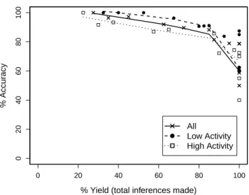
Fig. 2. Hunch: Accuracy vs. yield for simulated users: average of 8 users, 4 users assigned low-activity questions, 4 users assigned high-activity questions, thresholdscore ranges from 40% to 75%,thresholdsupport ranges between 28% and 55% of AUX size.
10 15 20 25 30
0
20
40
60
80
100
AUX Size
% Y
ield
●
● ●
● ●
● ●
● ●
● ● ● ●
● ● ● ●
● ● ● ● ● ●
● Correct Inferences Total Inferences
Fig. 3. Hunch: Yield vs. size of AUX for simulated users.thresholdscore is 70%,thresholdsupportis 51.25% of AUX size.
following the actual distribution obtained from Hunch, e.g., if 42% of real users respond “North America” to some question, then the simulated user selects this answer with0.42 probability. Results are in Fig. 2. As expected, the inference algorithm performs better on less active questions. Overall, our algorithm achieves 78% accuracy with 100% yield.
Fig. 3 shows, for a particular setting of parameters, how yield and accuracy vary with the size of auxiliary information. As expected, larger AUX reduces the number of incorrect
0
1
2
3
4
5
6
7
8
9
10
A B C D E G H I
Average
Number Correct
User
Bayesian Predictor
Inference Algorithm
Fig. 4. Inference vs. Bayesian prediction on simulated Hunch users.
thresholdscoreis 55%,thresholdsupportis 40% of AUX size. We used low thresholds to ensure that our algorithm reached 100% yield.
inferences, resulting in higher accuracy.
Inference vs. prediction.To illustrate the difference between inference and prediction, we compared the performance of our algorithm to a Bayesian predictor. Let Xi be a possible
answer to a TARGET question andYj be the known response
to the jth AUX question. The predictor selects Xi to
max-imize P(Xi|Y1)P(Xi|Y2)· · ·P(Xi|Yn), where P(Xi|Yj) = P(XiYj)
P(Yj) =
covar(Xi,Yj)+P(Xi)P(Yj)
P(Yj) . Individual probabilities
and covariances are available from the Hunch API. As Fig. 4 shows, our algorithm greatly outperforms the Bayesian predic-tor, averaging 73.75% accuracy vs. 33.75% accuracy for the predictor. This is not surprising, because our algorithm is not making educated guesses based on what similar users have done, it is observing the effects of actual transactions!
B. LibraryThing
LibraryThing is an online recommender system for books with over 1 million members and 55 million books in their online “libraries” [19]. For each book, LibraryThing provides a “People with this book also have... (more common)” list and a “People with this book also have... (more obscure)” list. These lists have 10 to 30 items and are updated daily.
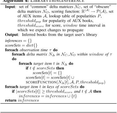
Algorithm 4 shows our inference procedure. Here delta matrices contain changes in “related books (common)” and “related books (obscure)” lists. Because these lists are updated frequently, the algorithm takes a window parameter. When a book is added to the user’s library, we expect that, within window, it will rise in the lists associated with the “auxiliary” books. Algorithm 5 counts the number of such lists, provided they are associated with less popular auxiliary books.
We used the site’s public statistics to select 3 users who had consistently high activity, with 30-40 books added to their collections per month. 200 random books from each user’s collection were selected as auxiliary information. The experiment ran for 4 months. Results are shown in Fig. 5.
Algorithm 4: LIBRARYTHINGINFERENCE
Input: set of “common” delta matricesNC, set of “obscure” delta matrices NO, scoring function:R|A|→ P(A), set
of AUX itemsA, lookup table of popularities P, thresholdpop for popularity of AUX books, thresholdscorefor score,windowtime interval in which we expect changes to propagate
Output: Inferred books from the target user’s library inferences={}
scoreSets=dict{}
foreachobservation timeτ do
foreachdelta matrixN∆ inNC,NO withinwindow ofτ do
foreachtarget itemtinN∆ do ift /∈scoreSetsthen
scoreSets[t] ={} scoreSets[t] =scoreSets[t]∪
SCOREFUNCTION(N∆[t],A, P, thresholdpop) foreachtarget itemtin keys ofscoreSetsdo
if|scoreSets[t]| ≥thresholdscoreandt /∈ Athen inf erences=inf erences∪ {t}
returninf erences
Algorithm 5: LTSCOREFUNCTION
Input: Delta-matrix rowTt corresponding to bookt,
implemented as a dictionary keyed on AUX books and containing the relative change in list position, set of AUX booksA, lookup table of popularities P, thresholdfor popularity of AUX book
Output: Subset of AUX books with whichtincreased in correlation
scoreSet={} foreacha∈ Ado
ifpopularityP[a]≤thresholdthen ifTt[a]>0then
scoreSet=scoreSet∪ {a} returnscoreSet
When parameters are tuned for higher yield, related-items inference produces many false positives for LibraryThing. The reason is that many public libraries have accounts on LibraryThing with thousands of books. Even if some book rises in K lists related to the target user’s library, K is rarely more than 20, and 20 books may not be enough to identify a single user. False positives often mean that another LibraryThing user, whose library is a superset of the target user’s library, has added the inferred book totheir collection.
C. Last.fm
Last.fm is an online music service with over 30 million monthly users, as of March 2009 [18]. Last.fm offers cus-tomized radio stations and also records every track that a user listens to via the site or a local media player with a Last.fm plugin. A user’s listening history is used to recommend music and is public by default. Users may choose not to reveal real-time listening data, but Last.fm automatically reveals the number of times they listened to individual artists and tracks. Public individual listening histories provide a “ground-truth oracle” for this experiment, but the implications extend to
0 10 20 30 40 50 60 70 80 90 100
0 10 20 30 40 50 60
%
A
c
c
u
ra
c
y
Yield (total inferences made) All Users
Strongest User
Fig. 5. LibraryThing: Accuracy vs. yield: for all users (averaged) and for the strongest user.
cases where individual records are private.
Aggregated data available through the Last.fm site and API include user-to-user recommendations (“neighbors”) and item-to-item recommendations for both artists and tracks. We focus on track-to-track recommendations. Given a track, the API provides an ordered list of up to 250 most similar tracks along with “match scores,” a measure of correlation which is normalized to yield a maximum of one in each list.
Our Last.fm experiment is similar to our LibraryThing experiment. Using changes in the similarity lists for a set of known auxiliary (AUX) tracks, we infer some of the TARGET tracks listened to by the user during a given period of time.
Unlike other tested systems, Last.fm updates all similarity lists simultaneously on a relatively long cycle (typically, every month). Unfortunately, our experiment coincided with changes to Last.fm’s recommender system.4Thus during our six-month experiment, we observed a single update after approximately four months. Batched updates over long periods make infer-ence more difficult, since changes caused by a single user are dominated by those made by millions of other users.
Several features of Last.fm further complicate adversarial inference. Last.fm tends not to publish similarity lists for unpopular tracks, which are exactly the lists on which a single user’s behavior would have the most impact. The number of tracks by any given artist in a similarity list is limited to two. Finally, similarity scores are normalized, hampering the algorithm’s ability to compare them directly.
Setup. We chose nine Last.fm users with long histories and public real-time listening information (to help us verify our inferences). As auxiliary information, we used the 500 tracks that each user had listened to most often, since this or similar information is most likely to be available to an attacker. Inferring tracks.After each update, we make inferences using
4Private communication with Last.fm engineer, July 2010.
TABLE I
ATTRIBUTES OF CANDIDATE INFERENCES. COMPUTED SEPARATELY FOR AUXITEMS FOR WHICHTARGETROSE AND THOSE FOR WHICH IT FELL.
Attribute Definition
numSupports Number of AUX similarity lists in which TARGET rose/fell
avgInitP os Average initial position of TARGET item in supporting AUX item similarity list
avgChange Average change of TARGET item in sup-porting AUX item similarity lists
avgListeners Average number of listeners for AUX items supporting TARGET
avgP lays Average number of plays for AUX items supporting TARGET
avgArtistScore Average number of other AUX supports by same artist as any given AUX support
avgSimScore Average sum of match scores for all other AUX supports appearing in any given AUX support’s updated similarity list
avgT agScore Average sum of cosine similarity between normalized tag weight vectors of any given AUX support and every other AUX support
the generic algorithm for related-items lists (Algorithm 1) with one minor change: we assume that each value in N∆ also
stores the initial position of the item prior to the change. Our scoring function could simply count the number of AUX similarity lists in which a TARGET track has risen. To strengthen our inferences, we use the scoring function shown in Algorithm 6. It takes into account information summarized in Table I (these values are computed separately for the lists in which the TARGET rose and those in which it fell, for a total of 16 values). To separate the consequences of individual actions from larger trends and spurious changes, we consider not only the number of similarity lists in which the TARGET rose and fell, but also the TARGET’s average starting position and the average magnitude of the change. Because the expected impact of an individual user on an AUX item’s similarity list depends on the popularity of the AUX item, we consider the average number of listeners and plays for AUX tracks as well.
We also consider information related to the clustering of AUX tracks. Users have unique listening patterns. The more unique the combination of AUX tracks supporting an inference, the smaller the number of users who could have caused the observed changes. We consider three properties of AUX supports to characterize their uniqueness. First, we look at whether supports tend to be by the same artist. Second, we examine whether supports tend to appear in each other’s similarity lists, factoring in the match scores in those lists. Third, the API provides weighted tag vectors for tracks, so we evaluate the similarity of tag vectors between supports.
To fine-tune the parameters of our inference algorithm, we use machine learning. Its purpose here is to understand the Last.fm recommender system itself and is thus very different from collaborative filtering—see Section V. For each target user, we train the PART learning algorithm [12] on all other target users, using the 16 features and the known correct or incorrect status of the resulting inference. The ability to
Algorithm 6: LASTFMSCOREFUNCTION
Input: Delta-matrix rowTt corresponding to itemt. Each vector entry containsinitP os- the initial position oft in the list, andchange- the number of placesthas risen or fallen in the list. We also assume that each AUX item is associated with
(listeners, plays, simList, tags)which are, respectively, the number of listeners, the number of plays, the updated similarity list with match scores, and the vector of weights for the item’s tags.
Output: Ascorefor the row score= 0
Arise={a∈Ttsuch thatTt[a][change]>0} Af all={a∈Tt such thatTt[a][change]<0} datarise= [0,0,0,0,0,0,0,0]
dataf all= [0,0,0,0,0,0,0,0] foreachrelevant∈ {rise, f all}do
numSupports=|Arelevant|
avgInitP os=avg(Tt[a][initP os]fora∈ Arelevant) avgChange=avg(Tt[a][change]fora∈ Arelevant) avgListeners=avg(a[listeners]fora∈ Arelevant) avgP lays=avg(a[plays]fora∈ Arelevant) avgArtistScore= 0
avgSimScore= 0 avgT agScore= 0
foreachaux itema∈ Arelevantdo
foreachaux itema06=ain Arelevantdo ifa[artist] ==a0[artist]then
avgArtistScore+ = 1
ifa0 ina[simList]then
simList=a[simList]
avgSimScore+ =simList[a0][matchScore] tags=norm(a[tags])
tags0=norm(a0[tags])
avgT agScore+ =cosineSim(tags, tags0)
ifnumSupports >0then
avgArtistScore=avgArtistScore/numSupports avgSimScore=avgSimScore/numSupports avgT agScore=avgT agScore/numSupports datarelevant= [numSupports, avgInitP os, avgChange, avgListeners, avgP lays, avgArtistScore, avgSimScore, avgT agScore]
if|Arise|>0then
score=MLPROBCORRECT(datarise, dataf all) returnscore
analyze data from multiple users is not necessary: a real attacker can train on auxiliary data for the target user over multiple update cycles or use his knowledge of the recom-mender system to construct a model without training. The model obtained by training on other, possibly unrepresentative users underestimates the power of the attacker.
After constructing the model, we feed the 16 features of each TARGET into the PART algorithm using the Weka machine-learning software [35]. Given the large number of incorrect inferences in the test data, Weka conservatively classifies most attempted inferences as incorrect. Weka also provides a probability that an inference is correct (represented by MLPROBCORRECT in Algorithm 6). We take these prob-abilities into account when scoring inferences.
We also account for the fact that similarity lists change in
0 20 40 60 80
0 500 1000 1500 2000
%
A
c
c
u
ra
c
y
Yield (total inferences made) Fig. 6. Accuracy vs. yield for an example Last.fm user.
0 10 20 30 40
0 500 1000 1500 2000
%
A
c
c
u
ra
c
y
Yield (total inferences made) Fig. 7. Accuracy vs. yield for another Last.fm user.
length and cannot contain more than two tracks by the same artist. For example, if a track was “crowded out” in a similarity list by two other tracks from the same artist, we know that its position was below the lowest position of these two tracks. Therefore, we judge the magnitude of any rise relative to this position rather than the bottom of the list. Similarly, if a list grows, we can confirm that a track has risen only if it rises above the bottom position in the previous list.
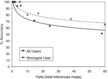
Results. The performance of our inference algorithm was negatively impacted by the fact that instead of a typical monthly update, it had to make inferences from a huge, 4-month update associated with a change in the recommender algorithm.5 Figs. 6 and 7 shows the results for two sample
users; different points correspond to different settings of the threshold parameter of the algorithm. For the user in Fig. 6, we make 557 correct inferences at 21.3% accuracy (out of 2,612 total), 27 correct inferences at 50.9% accuracy, and 7 correct inferences at 70% accuracy. For the user in Fig. 7, we make 210 correct inferences at 20.5% accuracy and 31 correct inferences at 34.1% accuracy.
5Last.fm’s changes to the underlying recommender algorithm during our experiment may also have produced spurious changes in similarity lists, which could have had an adverse impact.
For a setting at which 5 users had a minimum of 100 correct inferences, accuracy was over 31% for 1 user, over 19% for 3 users, and over 9% for all 5 users. These results suggest that there exist classes of users for whom high-yield and moderate-accuracy inferences are simultaneously attainable.
D. Amazon
We conducted a limited experiment on Amazon’s recom-mender system. Without access to users’ records, we do not have a “ground-truth oracle” to verify inferences (except when users publicly review an inferred item, thus supporting the inference). Creating users with artificial purchase histories would have been cost-prohibitive and the user set would not have been representative of Amazon users.
The primary public output of Amazon’s recommender sys-tem is “Customers who bought this isys-tem also bought . . . ” isys-tem similarity lists, typically displayed when a customer views an item. Amazon reveals each item’s sales rank, which is a measure of the item’s popularity within a given category.
Amazon customers may review items, and there is a public list of tens of thousands of “top reviewers,” along with links to their reviews. Each reviewer has a unique reviewer identifier. Reviews include an item identifier, date, and customer opinions expressed in various forms. Customers are not required to review items that they purchase and may review items which they did not purchase from Amazon.
Setup. Amazon allows retrieval of its recommendations and sales-rank data via an API. The data available via the API are only a subset of that available via the website: only the 100 oldest reviews of each customer (vs. all on the website) and only the top 10 similar items (vs. 100 or more on the website). We chose 999 customers who initially formed a contiguous block of top reviewers outside the top 1,000. We used the entire set of items previously reviewed by each customer as auxiliary information. The average number of auxiliary items per customer varied between 120 and 126 during our experi-ment. Note that this auxiliary information is imperfect: it lacks items which the customer purchased without reviewing and may contain items the customer reviewed without purchasing. Data collection ran for a month. We created a subset of our list containingactivecustomers, defined as those who had written a public review within 6 months immediately prior to the start of our experiment (518 total). If a previously passive reviewer became active during the experiment, we added him to this subset, so the experiment ended with 539 active customers. For each auxiliary item of each active customer, we retrieved the top 10 most related items (the maximum permitted by the API)6daily. We also retrieved sales-rank data
for all items on the related-item lists.7
Making inferences. Our algorithm infers that a customer has purchased some target item tduring the observation period if 6The set of inferences would be larger (and, likely, more accurate) for an attacker willing to scrape complete lists, with up to 100 items, from the site. 7Because any item can move into and off a related-items list, we could not monitor the sales ranks of all possible target items for the full month. Fortunately, related-items lists include sales ranks for all listed items.
t appears or rises in the related-items lists associated with at least K auxiliary items for the customer. We call the corresponding auxiliary items the supporting items for each inference. The algorithm made a total of 290,182 unique (user, item) inferences based on a month’s worth of data; of these, 787 had at least five supporting items.
One interesting aspect of Amazon’s massive catalog and customer base is that they make items’ sales ranks useful for improving the accuracy of inferences. Suppose (case 1) that you had previously purchased item A, and today you purchased itemB. This has the same effect on their related-items lists as if (case 2) you had previously purchasedB and today purchased A. Sales rank can help distinguish between these two cases, as well as more complicated varieties. We expect the sales rank for most items to stay fairly consistent from day to day given a large number of items and customers. Whichever item was purchased today, however, will likely see a slight boost in its sales rank relative to the other. The relative boost will be influenced by each item’s popularity,e.g., it may be more dramatic if one of the items is very rare.
Case studies. Amazon does not release individual purchase records, thus we have no means of verifying our inferences. The best we can do is see whether the customer reviewed the inferred item later (within 2 months after the end of our data collection). Unfortunately, this is insufficient to measure accuracy. Observing a public review gives us a high confidence that an inference is correct, but the lack of a review does not invalidate an inference. Furthermore, the most interesting cases from a privacy perspective are the purchases of items for which the customer wouldnot post a public review.
Therefore, our evidence is limited to a small number of verifiable inferences. We present three sample cases. Names and some details have been changed or removed to protect the privacy of customers in question. To avoid confusion, the inferred item is labeled t in all cases, and the supporting auxiliary items are labeleda1,a2, and so on.
Mr. Smith is a regular reviewer who had written over 100 reviews by Day 1 of our experiment, many of them on gay-themed books and movies. Itemtis a gay-themed movie. On Day 20, its sales rank was just under 50,000, but jumped to under 20,000 by Day 21. Mr. Smith’s previous reviews included itemsa1,a2,a3, a4, and a5. Itemt was not in the
similarity lists for any of them on Day 19 but had moved into the lists for all five by Day 20. Based on this information, our algorithm inferred that Mr. Smith had purchased item t. Within a month, Mr. Smith reviewed item t.
Ms. Brown is a regular reviewer who had commented on several R&B albums in the past. Itemtis an older R&B album. On Day 1, its rank was over 70,000, but decreased to under 15,000 by Day 2. Ms. Brown had previously reviewed items a1, a2, and a3, among others. Item A moved into item a1
and item a2’s similarity lists on Day 2, and also rose higher
in item a3’s list that same day. Based on this information,
our algorithm inferred that Ms. Brown had purchased itemt. Within two months, Ms. Brown reviewed itemt.
Mr. Grant is a regular reviewer who appears to be interested in action and fantasy stories. Itemt is a fairly recent fantasy-themed movie. On Day 18, its sales rank jumped from slightly under 35,000 to under 15,000. It experienced another minor jump the following day, indicating another potential purchase. Mr. Grant’s previous reviews included items a1, a2, and a3.
On Day 19, itemtrose in the similarity lists ofa1anda2, and
entereda3’s list. None of the supporting items had sales rank
changes that indicate purchases on that date. Based on this information, our algorithm inferred that Mr. Grant had bought itemt. Within a month, Mr. Grant reviewed itemt.
In all cases, the reviewers are clearly comfortable with public disclosure of their purchases since they ultimately reviewed the items. Nevertheless, our success in these cases suggests a realistic possibility that sensitive purchases can be inferred. While these examples include inferences supported by items in a similar genre, we have also observed cross-domain recommendations on Amazon, and much anecdotal evidence suggests that revealing cross-domain inferences are possible. For example, Fortnow points to a case in which an Amazon customer’s past opera purchases resulted in a recom-mendation for a book of suggestive male photography [11].
VII. EVALUATION ON A SIMULATED SYSTEM To test our techniques on a larger scale than is readily feasible with the real-world systems that we studied, we performed a simulation experiment. We used the Netflix Prize dataset [28], which consists of 100 million dated ratings of 17,770 movies from 460,000 users entered between 1999 and 2005. For simplicity, we ignored the actual ratings and only considered whether a user rated a movie or not, treating the transaction matrix as binary. We built a straightforward item-to-item recommender system in which item similarity scores are computed according to cosine similarity. This is a very popular method and was used in the original published description of Amazon’s recommender system [21].
We restricted our simulation to a subset of 10,000 users who have collectively made around 2 million transactions.8
Producing accurate inferences for the entire set of 460,000 users would have been difficult. Relative to the total number of users, the number of items in the Netflix Prize dataset is small: 17,770 movies vs. millions of items in (say) Amazon’s catalog. At this scale, most pairs of items, weighted by popularity, have dozens of “simultaneous” ratings on any single day, making inference very challenging.
Methodology.We ran our inference algorithm on one month’s worth of data, specifically July 2005. We assumed that each user makes a random 50% of their transactions (over their entire history) public and restricted our attention to users with at least 100 public transactions. There are around 1,570 such users, or 16%. These users together made around 1,510 transactions during the one-month period in question.
8Reported numbers are averages over 10 trials; in each trial, we restricted the dataset to a random sample of 10,000 users out of the 460,000.
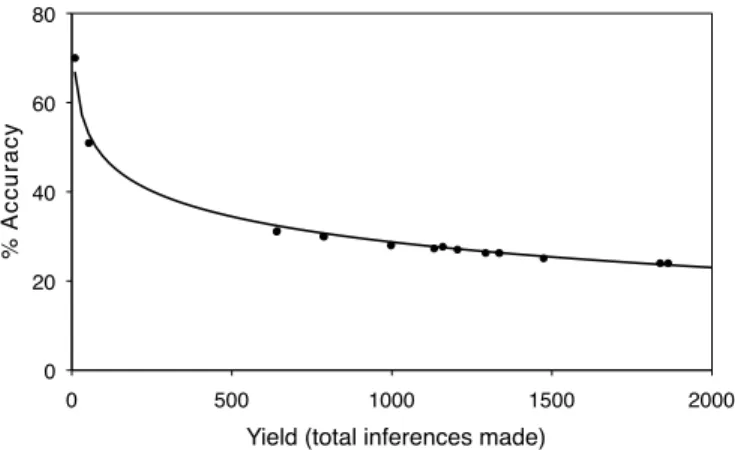
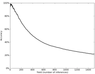
Fig. 8. Inference against simulated recommender: yield vs. accuracy.
We assume that each item has a public similarity list of 50 items along with raw similarity scores which are updated daily. We also assume that the user’s total number of transactions is always public. This allows us to restrict the attack to (customer, date) pairs in which the customer made 5 or fewer transactions. The reason for this is that some users’ activity is spiky and they rate a hundred or more movies in a single day. This makes inference too easy because guessing popular movies at random would have a non-negligible probability of success. We focus on the hard case instead.
Results. The results of our experiment are summarized in Fig. 8. The algorithm is configured to yield at most as many inferences as there are transactions: 1510/1570 ≈ 0.96 per vulnerable user for our one-month period. Of these, 22% are correct. We can trade off yield against accuracy by only outputting higher-scoring inferences. An accuracy of 80% is reached when yield is around 141, which translates to7.5%of transactions correctly inferred. At an accuracy level of90%, we can infer4.5%of all transactions correctly. As mentioned earlier, these numbers are averages over 10 trials.
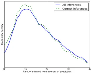
Inference vs. prediction. Fig. 9 shows that transactions involving obscure items are likely to be inferred in our simu-lated experiment. Fig. 10 shows that our inference algorithm accurately infers even items that a predictor would rank poorly for a given user. For this graph, we used a predictor that maximizes the sum-of-cosines score, which is the natural choice given that we are using cosine similarity for the item-to-item recommendations. The fact that the median prediction rank of inferred items lies outside the top 1,000 means, intuitively, that we arenot simply inferring the items that the user is likely to select anyway.
VIII. MITIGATION
Differential privacy.Differential privacy is a set of algorithms and analytical techniques to quantify and reduce privacy risk