Numerical Solution of the System of Nonlinear Fredholm Integro-Differential Equations by the Operational Tau Method with an Error Estimation

Numerical Solution of the System of

Nonlinear Fredholm Integro-Dierential

Equations by the Operational Tau

Method with an Error Estimation

G. Ebadi

, M.Y. Rahimi

1

and S. Shahmorad

1

In this paper, the operational approach to the Tau method is used for the numerical solution of a nonlinear Fredholm integro-dierential equations system and nonlinear ODEs with initial or boundary conditions without linearizing. An ecient error estimation of the approximate solution is also introduced. Some examples are given to clarify the eciency and high accuracy of the method.

INTRODUCTION

In recent years, the operational approach to the Tau method has been developed to cover the numerical solution of ODEs, PDEs and linear integro-dierential equations [1-10]. Liu and Pan presented an extension of the operational approach to the Tau method for the numerical solution of a linear ODEs system with polynomial or rational polynomial coecients, together with initial or boundary conditions [11]. Ortiz et al. have solved nonlinear ODEs and PDEs using an operational approach to the Tau method, through an iteration process dened by a sequence of linear problems with variable coecients [1,4,5,8].

In this paper, Ortiz and Samara's operational approach to the Tau method is considered for the numerical solution of nonlinear ODEs and nonlinear Fredholm integro-dierential equations system without linearizing.

Consider the following nonlinear Fredholm integro-dierential equations system:

m

X

j=1

Dijyj(x) i

Z b

a ki(x;t)'i(y1(t);

;yn(t))dt

=fi(x);

i= 1(1)m; x2[a;b]; (1)

*. Corresponding Author, Faculty of Mathematical Science, University of Tabriz, Tabriz, I.R. Iran.

1. Faculty of Mathematical Science, University of Tabriz, Tabriz, I.R. Iran.

with the supplementary conditions:

m

X

j=1

n_dj

X

k=1

(Ajkry(k 1)

j (a) +Bjkry(k 1)

j (b)) =dr;

r= 1(1)!; (2)

where:

[ndj = max1im

fndijg; !=

m

X

j=1

ndj];

and:

2 4Dij =

n_dij

X

r=0

pijr(x)_dxdr_r = n_dij

X

r=0

ijr

X

s=0

pijrsxs_dxdr_r

3 5:

For i = 1(1)m, fi(x) and ki(x;t) are polynomials in

x and inx,t, respectively and'i(y1(t);

;yn(t)) are

polynomials iny1(t);

;yn(t), otherwise, they can be

approximated by polynomials with suitable methods andijr is degree ofpijr(x).

In this paper, one assumes that, for i, j = 1(1)m, ij 2

N

, 'i(y

1(t);

;yn(t)) = Qm

j=1y

ij

j (t),

otherwise, it can be written as a sum of this form by a suitable method, for example, Taylor expansion.

The organization of this paper is as follows: First, the operational approach to the Tau method for the numerical solution of Fredholm Integro-Dierential Equations (FIDEs) is explained. Then, the numerical solution of a linear FIDEs system by the Tau method is reviewed, and the operational approach to the Tau

method is applied to a nonlinear FIDEs system. After that, the nonlinear ODEs are solved and an error function is introduced. Some numerical results are given, also, to clarify the accuracy of the method and, nally, the contains conclusions are presented. Note that, the numerical results are computed by Maple programming.

Remark 1

Fori= 1(1)m, the following notations have been used throughout this paper:

x= (1;x;x2; )T;

xa = (1;a;a2; )T;

xb = (1;b;b2; )T;

e1= (1;0;0; )T;

y_in= (yi0;yi1;

;yin;0;)T;

fi= (fi0;fi1;

;fin

fi;0;)T;

f = (f0;f1;

;fnf;0;)T;

y_n= (y0;y1;

;yn;0;)T:

LINEAR AND NONLINEAR FIDES

The operational approach to the Tau method describes the reduction of given linear and nonlinear integro-dierential equations (IDEs) to a linear and nonlinear algebraic equations system, based on three simple matrices:

=

0 B B B B B @

0 1 0 0 0 1 0

0 1 ... 0 :::

1 C C C C C A

;

=

0 B B B B B @

0 1 0

0 2 0 ...

0 0 3 0 :::

1 C C C C C A

;

=

0 B B B B B @

0 1 0 0

0 1

2 0

0 1

3 ...

0 :::

1 C C C C C A

:

Linear FIDEs

Consider the linear FIDEs (the following result is quoted from [1,9,11]):

Dy(x) Z b

a k(x;t)y(t)dt=f(x); x2[a;b]; (3)

with the supplementary conditions:

nd

X

k=1

(Akjy(k 1)(a) +B

kjy(k 1)(b)

=dj;

j= 1(1)nd; (4)

where: D=Xnd

i=0

pi(x)_dxdi_i =Xnd

i=0

i

X

j=0

pijxj_dxdi_i;

is the dierential operator of ordernd.

Letyn(x) =Pn

j=0yjx

j _{=ynTx, then:}

xr_{yn(x) =}Xn

j=0

yjxj+r=y

nTrx;

and: y(r)

n (x) = _dxdrryn(x) =ynTrx: (5)

Theorem 1

Let yn(x) = ynTx 2 Cnd[a;b]; (the space of nd-times

continuously dierentiable functions on [a;b]) and: D=Xnd

i=0

pi(x)_dxdi_i =Xnd

i=0

i

X

j=0

pijxj_dxdi_i;

be a linear dierential operator of order nd with

polynomial coecients, then;

Dyn(x) =ynTx; (6)

where: =Xnd

i=0

i_{pi() =}Xnd

i=0

i

X

j=0

pijij:

Theorem 2

If k(x;t) = Pn

i=0 Pn

j=0kijx

i_tj_{, kij} 2

R

and y(x) =

y_nTx, then:

Z b

a k(x;t)y(t)dt=ynTfx; (7)

where f = Pn

i=0 Pn

j=0kij

ij

f is a matrix associated

uniquely withk(x;t) and constantsa;b, such that,ij_f = j_{(xb xa)e}

1

Lemma 1

Ifyn(x) =ynTx, then,

y(k)

n (a) =ynTkxa;

y(k)

n (b) =ynTkxb: (8)

Proof

By using Equation 5 one has: y(k)

n (a) =y(k)

n (x)jx

=a =ynT

k_xjx

=a=ynT

k_xa;

and: y(k)

n (b) =y(k)

n (x)jx

=b=ynT

k_xjx

=b=ynT

k_xb;

so, the proof is completed.

Applying Lemma 1 for supplementary Condi-tions 4, one has:

nd

X

k=1

Akjy(k 1)(a) +B

kjy(k 1)(b)

=Xnd

k=1

AkjynT(k 1)x

a+BkjynT(k 1)x

b

=y_nTXnd

k=1

Akj(k 1)x

a+Bkj(k 1)x

b

: Let:

Ej=Xnd

k=1

Akj(k 1)x

a+Bkj(k 1)x

b

; thus, Ej 2

M

(n+1)(1) and Equation 4 is converted

intoynTEj=dj,j= 1(1)nd.

Now, by using Equations 6 through 8, the integro-dierential Equation 3 and supplementary Conditions 4 reduce to the following algebraic equations system:

(

y_nTf =fT

ynTE=dT (9)

with f = f and:

E= (E1;E2;

;End)2

M

(n+1)(nd): (10)

By settingG= (E;f) andgT = (dT,fT), Equation 9

can be written asy_nTG = gT_{. To obtain yn(x), the}

system of equationsynTGn =gnT must be solved for

the unknown coecients, y0;y1;

;yn, where Gn is

the matrix dened by considering the rst (n+1) rows and columns of G; and gn is the vector dened by

considering the rst (n+ 1) elements of the vector,g.

Nonlinear FIDEs

Consider the nonlinear Fredholm integro-dierential equation:

Dy(x) Z b

a k(x;t)'(y(t))dt=f(x);x2[a;b];

(11) with the supplementary Conditions 4, where D is dened as before and'(y(t)) is a polynomial in y(t), otherwise, it is approximated by a polynomial with suitable methods. In this paper,'(y(t)) =ym_(t);m2

N

, is considered, since other types of '(y(t)) can be reduced to the sum of this form.

Theorem 3

If u(x) = Pm

j=0ujx

j _=uT_{x and v(x) =} Pm

i=0vix

i ₌

vT_{x, then, u(x)v(x) = u}T_{v()x, where v() =}

Pn

i=0vi

i_.

Proof

See [9].

Lemma 2

Lety(x) =y_nTx, then,ym_{(x) =ynTy}m 1()x. Proof

Letu(x) =y_nTx and v(x) =ym 1(x) and Theorem 3

be applied.

Theorem 4

If yn(x) = Pn

i=0yinx

i _{= ynTx and k(x;t) =}

Pn

i=0 Pn

j=0kijx

i_tj_{, then,}

Z b

a k(x;t)ymn(t)dt=ynTfmx; (12)

where fm =ym 1

n ()f andf is the same matrix as

introduced in Theorem 2.

Proof

Use Lemma 2 and Theorem 2 for y(x) = ynTym 1()x.

If Equations 6, 10 and 12 are used for: Dy(x) Z b

a k(x;t)ym(t)dt=f(x); x2[a;b];

m2

N

;

with supplementary Conditions 4, the following nonlin-ear system will be obtained:

(

ynTf =fT;

y_nTE=dT; (13)

where f = fm and fm is the same matrix

and gT _{= (d}T_;fT_{), one has y}T_{G = g}T _{instead of}

Equation 13, which is a nonlinear algebraic equations system, because Gcontains unknown elements of the vector y_n. To nd yn(x), the nonlinear equations

systemynTGn=gnT must be solved, whereGnandgn

are dened by considering the (n+1)(n+1) leading

submatrix of G and the rst (n+ 1) elements of the vectorg, respectively.

LINEAR FIDES SYSTEM

Consider the system of linear FIDEs:

m

X

j=1

Dijyj(x) ij

Z b

a kij(x;t)yj(t)dt

!

=fi(x);

x2[a;b]; i= 1(1)m; (14)

with the supplementary Conditions 2, whereDij,i;j=

1(1)m, are the same as that in Equation 1, fi(x) =

Pnfi

j=0fijx

j _{= fi}T_{x. Now, applying Equations 6}

through 8, for Equations 14 and 2, they are converted into a system of linear algebraic equations. Let yjn(x) = yjnTx j = 1(1)m, be the Tau approximates

and let ij,i;j= 1(1)mdenote the matrices associated

with Dij, i;j = 1(1)m by Theorem 1 and fij, i;j =

1(1)m be the matrices associated with kij(x;t);i;j =

1(1)mby Theorem 2. Then, one has:

m

X

j=1

Dijyjn(x) ij

Z b

a kij(x;t)yjn(t)dt

!

=Xm

j=1

y_jnTijx ijyjnTfijx

=Xm

j=1

yjnT ij ijfij

x =Xm

j=1

yjnTijx; i= 1(1)m;

where:

ij = ij ijfij: (15)

Applying Lemma 1 to supplementary conditions:

m

X

j=1

n_dj

X

k=1

Ajkry(k 1)

j (a) +Bjkry(k 1)

j (b)

=dr;

r= 1(1)!;

yields:

m

X

j=1

n_dj

X

k=1

AjkryjnTk 1x

a+BjkryjnTk 1x

b

=Xm

j=1

y_jnTXndj

k=1

Ajkrk 1x

a+Bjkrk 1x

b

=dr:

Assume that:

n_dj

X

k=1

Ajkrk 1x

a+Bjkrk 1x

b

=Erj2

M

(n+1)(1);

then, one has:

m

X

j=1

y_jnTErj=dr;r= 1(1)!;

and:

m

X

j=1

y_jnTEj=dT;

with:

Ej= (E1j;E2j;E2j;

;E!j);

and:

dT = (d1;d2;d3;

;d!):

LetyMT = (y1nT;y2nT;y3nT;

;ymnT)2

R

M,M =

m(n+ 1), where yjnT, j = 1(1)m are the coecients

vectors of yjn(x) in a standard basis. The problem

of determining y_MT can be formulated as the linear equations system [11]:

y_MT

G

=SMT; (16)

with:

G

=

0 B B B @

E1 Q11 Q21

Qm 1

E2 Q12 Q22

Qm 2

... ... ... ... ...

Em Q1m Q2m

Qmm 1 C C C A 2

M

m

(n+1)m(n+1);

where Qij = (ij)(n+1)(n ndi+1) is the restriction of

ij (as dened in Equation 15) to its rst (n+1) rows

and (n ndi+ 1) columns and:

SMT = (dT;f1nd 1

T_;f

2nd 2

T_;

;fmn

dmT)2

R

M;

where f_indiT is the restriction of f_iT to its rst (n ndi + 1) components. By solving Equation 16,

NONLINEAR FIDES SYSTEM

Consider the nonlinear FIDEs system:

m

X

j=1

Dijyj(x) i

Z b

a ki(x;t) m

Y

j=1

y_jij_(t)dt=fi(x);

x2[a;b]; i= 1(1)m; (17)

with the supplementary conditions:

m

X

j=1

n_dj

X

k=1

Ajkry(k 1)

j (a) +Bjkry(k 1)

j (b)

=dr;

r= 1(1)!; where:

ndj = max

1im

fndijg; !=

m

X

j=1

ndj;

Dij = n_dij

X

r=0

pijr(x)_dxdr_r = n_dij

X

r=0

ijr

X

s=0

pijrsxs_dxdr_r;

for i;j = 1(1)m;ndij is the order of operator

Dij;fi(x);ki(x;t) are algebraic polynomials in x and

x;t, respectively, and;a;bare given constants.

Lemma 3

Letyi(x) =yinTx;i= 1(1)m then: m

Y

i=1

yr_ii_{(x) =y}

1nTy

r1 1 1 ()

m

Y

i=2

yr_ii_{()x; ri} 2

N

: Proof

One has:

m

Y

i=1

yr_ii_{(x) =y}

1(x)y

r1 1 1 (x)

m

Y

i=2

yr_ii_(x);

if one sets: v(x) =yr1

1 1 (x)

m

Y

i=2

yr_ii_{(x); u(x) =y}

1(x);

then, by using Theorem 3, the proof is completed.

Theorem 5

If k(x;t) = Pn

i=0 Pn

j=0kijx

i_tj _{with kij} 2

R

;i;j =

1(1)mand yj(x) =yjnTx;j = 1(1)m, then:

Z b

a k(x;t) m

Y

i=s

y_iri_{(t)dt=ysnTfsx;}

where: fs=yrs 1

s () m

Y

i=s+1

yr_ii₍₎Xn

i=0

n

X

j=0

kijj(xb xa)e1

Ti_;

is a matrix associated uniquely withk(x;t).

Proof

Using Theorem 2 with y(x) = Pm

i=sy

ri

i (x) =

y_snTyrs 1

s ()Qm

i=s+1y

ri

i ()x and setting ynT =

y_snTyrs 1

s ()Qm

i=s+1y

ri

i (), the proof is completed.

Let yjn(x) = yjnTx, j = 1(1)m be the Tau

approximations, then for i = 1(1)m;1 x b, one

has:

m

X

j=1

Dijyjn(x) i

Z b

a ki(x;t) m

Y

r=s

y_rnir_(t)dt

=Xm

j=1

y_jnTijx iysnTfsx

=Xm

j=1

y_jnTijx;

where: ij =

(

ij j 6=s

is isfs j =s; (18)

fi(x) =Pnfi

j=0fijx

j _=fiT_{xands= min}f1;;mgfor

whichis6= 0.

In the same way as done in the previous section, one has Pm

j=1yjnTEj = d

T _{instead of Equation 2.}

For determining the Tau approximations yjn(x) =

yjnTx;j = 1(1)m, Equations 17 and 2 are converted

into the system of nonlinear algebraic equations:

yMT

G

=SMT; (19)

where yMT and SMT are the same notations as used

in Equation 16 and:

G

=

0 B B B @

E1 Q11 Q21

Qm 1

E2 Q12 Q22

Qm 2

... ... ... ... ... Em Q1m Q2m

Qmm 1 C C C A 2

M

m

(n+1)m(n+1);

withQij= (ij)(n+1)(n ndi+1), which is the restriction

of ijto its rst (n+1) rows and (n ndi+1) columns.

It should be noted that, in Equation 18, the elements of is contain the unknown coecients ofyjn(x);j =

1(1)m. By solving the nonlinear system (Equation 19), one nds the unknown coecients of yjn(x) for j =

1(1)m.

NONLINEAR ODES

In this section, the nonlinear dierential equation f(x;y;y0;y00) = 0 is considered, wheref is an analytic

function in terms of y;y0 and y00. Therefore, the

equation can be written as: f(x;y;y0;y00) =

r

X

i=0

pi(x)yni(y0)mi(y00)qi = 0;

where r;ni;mi;qi 2

N

S

f0g and pi(x) is an analytic

function in terms ofx. Using Theorem 3 and Lemma 3, one can write:

f(x;y;y0;y00) =

r

X

i=0

y_nT(y())ni 1(y0())mi

(y

00())qip

i()x= 0Tx;

or: y_nTXr

i=0

(y())ni 1(y0())mi(y00())qip

i() = 0T; (20)

where 0T _{= (0};0)

(1)(n+1). Equation 20 and the

supplementary Conditions 4 form a system of nonlinear algebraic equations. Each equation of this system is a polynomial, in terms of unknown elements of vectoryn.

ESTIMATION OF ERROR FUNCTION

In this section, an error function is obtained for the approximate solution of Equations 2 and 17. Let ejn(x) =yj(x) yjn(x),j= 1(1)mbe called the error

function of Tau approximationyjn(x) toyj(x), where

yj(x), j = 1(1)m is the exact solution. Substituting

yj(x) = ejn(x) +yjn(x), j = 1(1)m in Equations 2

and 17, forx 2[a;b], i= 1(1)mand s2

N

, they can

be written as:

m

X

j=1

Dij(yjn(x) +ejn(x)) i

Z b

a ki(x;t) m

Y

j=s

(yjn(t)

+ejn(t))ij(t)dt=fi(x); (21)

and:

m

X

j=1

n_dj

X

k=1

Ajkr(yjn(a) +ejn(a))(k 1)

+Brjk(yjn(b) +ejn(b))(k 1) !

=dr;

r= 1(1)!:

By using (yjn(t) +ejn(t))p=Pp

k=0

k p

y_jnp k(t)ekjn(t) in Equation 21 and because of satisfying yjn(x) in

Equation 2, forx25[a;b] andi= 1(1)m, one has:

m

X

j=1

Dijejn(x) i

Z b

a ki(x;t)'i

esn(t);e(s+1)n(t);

;emn(t)

dt= Hin(x);

and:

m

X

j=1

n_dj

X

k=1

Ajkre(k 1)(a) +B

jkre(k 1)

jn (b)

= 0; r= 1(1)!;

where:

Hin(x) =Xm

j=1

Dijyjn(x) i

Z b

a ki(x;t) m

Y

j=s

y_jnij_(t)dt

fi(x);i= 1(1)m;

are the perturbation terms associated withyjn(x);j=

1(1)mand:

'i(esn(t);e(s+1)n(t);

;emn(t))

='1is

m

Y

j=s+1

(y_jnij_{(t) +'}

1ij)

+m 2 X

r=s

r

Y

j=s

y_jnij_(t)

'1i(r+1)

m

Y

j=r+2

(y_jnij_{(t) +'}

1ij)

+ m 1 Y

j=s

y_jnij_(t)

'1im;

with: '1ij=

ij

X

p=1

ij

p

y_jnij p_(t)epjn(t);

j=s(1)m; i= 1(1)!:

One proceeds to nd approximations ejn;N(x) to the

error functions, ejn(x), for j = 1(1)m and N 2

N

,

in the same way as done before for solving problem in Equations 17 and 2. With problems in Equations 17 and 2, the Tau problem:

m

X

j=1

Dijejn(x) i

Z b

aki(x;t)'i

esn(t);e(s+1)n(t); ;

emn(t)

was associated for i = 1(1)m;a x b; with the

supplementary conditions:

m

X

j=1

n_dj

X

k=1

Ajkre(k 1)(a) +B

jkre(k 1)

jn (b)

= 0; r= 1(1)!;

which denes ejn;N(x) forj = 1(1)m, whereN is the

degree of error polynomialejn(x).

NUMERICAL EXAMPLES

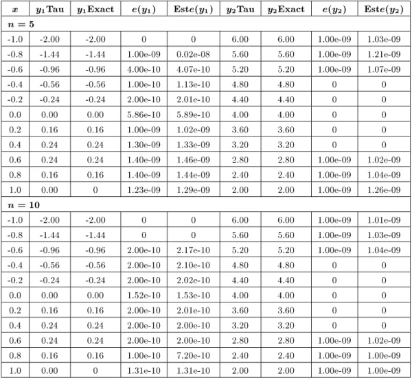
In this section, the eciency of the presented method is shown by some numerical results. Numerical results for Examples 1 to 3, were reported in Tables 1 and 2. In these tables, the terms yiTau, yiExact, e(yi) and

Est. e(yi) stand for Tau approximations ofyi(x), exact

solution, yi(x), their absolute error and estimation

error of yi for i = 1;2: It should be noted that, in

the following examples,N =n+ 2 has been used.

Example 1

Consider the following system of nonlinear FIDEs with the exact solutions,y1(x) =x x

2andy

2(x) = 4 2x.

y00 1(x) +x

2y0

1(x) + 3y

1(x) +y 0

2(x) 4y 2(x) Z

1 1

(3y2

1(t) + 2xy

1(t)y2(t))dt=f1(x);

y0

1(x) 2y

1(x) +y 00

2(x) 2y 0 2(x) +y

2(x) Z

1 1

((t x)y1(t) + 5t 2y2

2(t))dt=f 2(x);

with the supplementary conditions: y1( 1) +y

0

1( 1) = 1; y

1(1) +y 0

1(1) = 1;

y2( 1) +y 0

2( 1) = 4; y

2(1) +y 0

2(1) = 0:

where f1(x) = 116

5 + 19x 2x

2 2x3 and f 2(x) =

53 20 3x+2x

2. For the numerical results, see Table 1. Table1. Numerical results of Example 1.

x y1Tau y1Exact e(y1) Este(y1) y2Tau y2Exact e(y2) Este(y2) n=5

-1.0 -2.00 -2.00 0 0 6.00 6.00 1.00e-09 1.03e-09 -0.8 -1.44 -1.44 1.00e-09 0.02e-08 5.60 5.60 1.00e-09 1.21e-09 -0.6 -0.96 -0.96 4.00e-10 4.07e-10 5.20 5.20 1.00e-09 1.07e-09 -0.4 -0.56 -0.56 1.00e-10 1.13e-10 4.80 4.80 0 0 -0.2 -0.24 -0.24 2.00e-10 2.01e-10 4.40 4.40 0 0 0.0 0.00 0.00 5.86e-10 5.89e-10 4.00 4.00 0 0 0.2 0.16 0.16 1.00e-09 1.02e-09 3.60 3.60 0 0 0.4 0.24 0.24 1.30e-09 1.33e-09 3.20 3.20 0 0 0.6 0.24 0.24 1.40e-09 1.46e-09 2.80 2.80 1.00e-09 1.02e-09 0.8 0.16 0.16 1.40e-09 1.44e-09 2.40 2.40 1.00e-09 1.04e-09 1.0 0.00 0 1.23e-09 1.29e-09 2.00 2.00 1.00e-09 1.26e-09

n=10

-1.0 -2.00 -2.00 0 0 6.00 6.00 1.00e-09 1.01e-09 -0.8 -1.44 -1.44 0 0 5.60 5.60 1.00e-09 1.03e-09 -0.6 -0.96 -0.96 2.00e-10 2.17e-10 5.20 5.20 1.00e-09 1.04e-09 -0.4 -0.56 -0.56 2.00e-10 2.10e-10 4.80 4.80 0 0 -0.2 -0.24 -0.24 2.00e-10 2.02e-10 4.40 4.40 0 0 0.0 0.00 0.00 1.52e-10 1.53e-10 4.00 4.00 0 0 0.2 0.16 0.16 2.00e-10 2.01e-10 3.60 3.60 0 0 0.4 0.24 0.24 2.00e-10 2.00e-10 3.20 3.20 0 0 0.6 0.24 0.24 2.00e-10 2.00e-10 2.80 2.80 1.00e-09 1.02e-09 0.8 0.16 0.16 1.00e-10 7.20e-10 2.40 2.40 1.00e-09 1.00e-09 1.0 0.00 0 1.31e-10 1.31e-10 2.00 2.00 1.00e-09 1.00e-09

Example 2

Consider the nonlinear FIDEs system: y1(x) + 3xy2(x)

Z 1 2 0

(xty2 1(t) +t

2y3 2(t))dt

= 19 + 34x+ 3x3;

x2y

1(x) y2(x) Z

1 2 0

(ty3

1(t) xy 2(t))

2dt

= 19 + 27x 65x2+x3;

with exact solutiony1(x) =xandy2(x) =x

2. Table 2

presents the numerical results.

Example 3

Consider the nonlinear ODE: xy02 2yy0+x= 0;

with the supplementary condition y(0) = 1

2 and exact

solution y(x) = 1 2(x

2+ 1). For n = 4, the presented

method gives the system of nonlinear equations:

8 > > > > > > < > > > > > > :

y0= 1=2

2y0y1= 0

4y0y2 y 2 1= 1

6y0y3 2y1y2= 0

8y0y4 2y1y3= 0

; which has the solutionfy

0=y2= 0:5;y1=y3 =y4=

0gand leads toyn(x) = 0:5+0:5x

2and this is the exact

solution. For n = 7, one has the system of nonlinear equations:

8 > > > > > > > > > > > > > < > > > > > > > > > > > > > :

y0= 1=2

2y0y1= 0

6y0y3 2y1y2= 0

4y0y2 y 2 1= 1

8y0y4 2y1y3= 0

10y0y5 2y1y4+ 2y3y2= 0

12y0y6 2y1y5+ 3y 2 3+ 4y

4y2= 0

14y0y7 2y1y6+ 10y3y4+ 6y5y2= 0

and its solution isfy

0=y2= 0:5;y1=y3=y4=y5=

y6=y7= 0

g, which leads to the exact solution.

CONCLUSION

Nonlinear FIDEs systems are usually dicult to solve analytically, therefore, one needs to nd an approxi-mate solution. It has been shown that the operational approach to the Tau method is a suitable method of high accuracy for these problems.

The advantages of this method are, as follows: 1. It solves Nonlinear FIDEs systems and nonlinear

ODEs without linearization;

2. It gives an error estimator as a polynomial and improves accuracy by increasingnreasonably. In Tables 1 and 2, one can see that the accuracy of the Tau method at the end points of the intervals is less than the others. The authors will try to improve this in the future.

Table2. Numerical results of Example 2.

x y1Tau y1Exact e(y1) Este(y1) y2Tau y2Exact e(y2) Este(y2) n=5

0.0 0.00 0 2.170e-06 2.175e-06 0.00 0 2.170e-07 2.174e-07 0.1 0.10 0.10 1.797e-06 1.801e-06 0.01 0.01 3.765e-06 3.782e-06 0.2 0.20 0.20 3.352e-05 3.382e-05 0.04 0.04 1.192e-06 1.199e-06 0.3 0.30 0.30 4.990e-05 4.997e-05 0.09 0.09 3.512e-06 3.529e-06 0.4 0.39 0.40 6.818e-05 6.851e-05 0.16 0.16 7.563e-06 7.913e-06 0.5 0.49 0.50 8.945e-04 8.973e-04 0.25 0.25 1.432e-05 0.920e-04

n=10

0.0 0.00 0 2.170e-09 2.200e-09 0.00 0 2.170e-10 2.300e-10 0.1 0.10 0.10 2.101e-09 2.152e-09 0.01 0.01 7.494e-09 7.498e-09 0.2 0.20 0.20 6.997e-08 6.997e-08 0.04 0.04 2.294e-09 2.311e-09 0.3 0.30 0.30 1.828e-08 1.860e-08 0.09 0.09 4.275e-09 4.278e-09 0.4 0.40 0.40 4.837e-08 4.851e-08 0.16 0.16 5.634e-09 5.642e-09 0.5 0.50 0.50 7.004e-07 7.302e-07 0.25 0.25 5.808e-08 7.116e-08

ACKNOWLEDGMENT

The authors would like to thank the referee(s) for their careful considerations and valuable suggestions.

REFERENCES

1. Ortiz, E.L. and Samara, H. \An operational approach to the Tau method for the numerical solution of nonlinear dierential equations", Computing, 27, pp

15-25 (1981).

2. \Numerical solution of partial dierential equations with variable coecients with an operational approach to the Tau method",Comput. Math. Appl.,10(1), pp

5-13 (1984).

3. Rodrigues, M.J. and Matos, J. \Numerical solution of partial dierential equations with the Tau method", Departamento de Matematica de Universidade de Coimbra, Textos Matematica, Ser. B. 11, Fernanda Aragao Oliveira et al., Eds., pp 111-121 (1997). 4. Ortiz, E.L. and Pun, K.S. \Numerical solution of

nonlinear partial dierential equations with the Tau method",J. Comp. and Appl. Math., 12, pp 511-516

(1985).

5. Ortiz, E.L. and Aliabadi, M.H. \Numerical treatment of moving and free boundary value problems with the Tau method",Computers Math. Applic.,35(8), pp

53-61 (1998).

6. Pour-Mahmoud, J., Rahimi-Ardabili, M.Y. and Shah-morad, S. \Numerical solution of the system of Fredholm integro-dierential equations by the Tau method",Appl. Math. and Comput.,168, pp 465-478

(2005).

7. Ortiz, E.L. \The Tau method",SIAM J. Nume. Anal.,

6, pp 480-492 (1969).

8. \On the numerical solution of nonlinear and functional dierential equations with the Tau method", In Nu-merical Treatment of Dierential Equations in Appli-cations, Lecture Notes in Math., No. 679, Springer-Verlag, Berlin, pp 127-139 (1978).

9. Hosseini, S.M. and Shahmorad, S. \Numerical solution of a class of integro-dierential equations by the Tau method with an error estimation", Appl. Math. and Comput.,136, pp 550-570 (2003).

10. Shahmorad, S. \Numerical solution of a class of integro-dierential equations by the Tau method", Ph.D Thesis, Tarbiat Modarres University, Tehran, Iran (2002).

11. Liu, M.K. and Pan, C.K. \The automatic solution to systems of ordinary dierential equations by the Tau method",Computers and Mathematics with Applica-tions,17, pp 197-210 (1999).