Online dictionary learning for car recognition using sparse coding and LARS

ISSN: 2252-8938, DOI: 10.11591/ijai.v19i1.pp164-174 _r 164

Online dictionary learning for car recognition using sparse

coding and LARS

Ilias Kamal, Khalid Housni , Youssef Hadi

MISC Laboratory, Department of Computer Science, Faculty of Science,Ibn Tofail University,K´enitra, Morocco

Article Info Article history: Received Oct 10, 2019 Revised Jan 24, 2020 Accepted Feb 12, 2020 Keywords:

Car make and model recognition

Dictionary learning LARS

LASSO Sparse Coding

ABSTRACT

The bag of feature method coupled with online dictionary learning is the basis of our car make and model recognition algorithm. By using a sparse coding computing technique named LARS (Least Angle Regression) we learn a dictionary of codewords over a dataset of Square Mapped Gradient feature vectors obtained from a densely sampled narrow patch of the front part of vehicles. We then apply SVMs (Support Vector Machines) and KMeans supervised classification to obtain some promising results.

This is an open access article under theCC BY-SAlicense.

Corresponding Author: Ilias Kamal,

Department of Computer Science, Faculty of Science, Ibn Tofail University, B.P 133 Kenitra 14 000-Morocco. Tel: (+212)6 61 40 35 57

Email: [email protected]

1. INTRODUCTION

Vehicle make and model recognition systems (abbreviated VMMR) are part of intelligent transportation systems (abbreviated ITS), a field that has seen significant advances since the last twenty years. An intelligent transportation sytem is the integration of ”smart” communication and information processing technologies to the transportation system . Althought it usually encompasses all modes of transports, it is used to describe road, vehicle and driver interactions and aims to make them more dynamical, by enabling better and faster decision making for both road users and supervisers (if any). The push for better ITS and the massive investments made in it by countries like Japan or the USA naturally sowed the fields of innovation in all its related domains. Not only that but the gap in computational power, video-sensing and miniaturization technologies since the early nineties or even since the last decade continues to widens steadily, leading to more dense and powerful devices along with more sophisticated and performant VMMR software. The most widespread taxonomy of VMMR methods is split into two broad categories, namely appearance based and model based. Appearance based methods rely on photometric information and the features extracted from it (edges, corners,gradient...), whereas model based methods seek to obtain a good geometrical representation of the objects in the image often relying on stereo vision and two dimensionnal techniques for primitive extraction. Here we use the front part of the car which is considered to be the most discriminative [1–11], but different parts have been used too like a combination of different parts [12], the rear [13, 14], the logo [15] and even 3D modeling [16]. In this paper we build an appearance based VMMR system on the most discriminative part of the car located at the front using various feature extraction and classification techniques. We consider the VMMR problem in a bag of features framework that combines local

level features, sparse coding, dictionary learning and support vector machines (SVM). These local low-level features are used to form a global descriptor, which can be seen as a mid-low-level feature as mentioned in [17] and are also extensively used in deep neural networks [18, 19]. Sparse coding originaly used fixed dictionaries until Olshausen and Field [20, 21] where they used data to generate dictionaries representing an underlying hidden structure of said data. Raina et al. [22], compare PCA and sparse coding, building a dictionary using unlabeled images to obtain sparse representations of labeled images and feed them to a support vector machine. Yang et al. [23], build the dictionary from SIFT descriptor data instead of raw images and use a one-against-all multiclass linear SVM. In Zeiler et al. [24], a dictionary is built by stacking deconvolution and max pooling layers and uses conjugate gradients to update the filters (K filters for each layer) of the hierarchical dictionary, each deconvolution layer seeks to minimize the reconstruction error of an input image under a sparsity penalty. In general the aforementioned methods use the alternating or sequential optimization approach which updates either the dictionary or the coding matrix while fixing the other. More modern methods like Dir of Rakotomamonjy [25] jointly optmize the dictionary D and the coding matrix A which improves the algorithm runtime.

2. THE BAG OF FEATURES METHOD

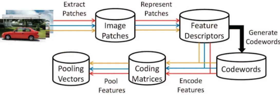
The general bag of features framework follows the six steps detailed below and shown in Figure 1. The bag of features although supervised by nature (the use of SVMs) relies more or less exclusively on a unsupervised learning method to generate said features in its argualbly most important step, i.d. the dictionary generation or learning step. Dictionary learning can be seen as matrix factorization problem along side other methods such as principal component analysis (PCA), clustering or vector quantization [26, 27], non-negative matrix factorization (NMF) [28, 29], archetypal analysis [30], or independent component analysis (ICA) [31–34].

Figure 1. Bag of features framework 2.1. Patch extraction

To streamline the process of extracting the relevant image patches as seen, we use [35] algorithm as illustrated in Figure 2. Simple and straightforward it is based on the use of horizontal gradient, morphological operations and connected component analysis to solve the license plate location in the image, which in turn enables us to obtain the front part of the vehicle for further processing.Then we sample local areas of the image patches acquired previously either densely [36, 37] or sparsely [38–40]. In our implementation we choose to use dense grid coverage of 2x2, 4x4, 8x8 or 16x16 patches over the image with no scaling and because of the tight segmentation, background clutter is kept to a strict minimum. However there are better sampling methods as pointed out by Nowak et al. [41] than dense sampling, many regions of the image have low discriminative power (most of them in fact) which hurts the performance.

Input image

Gradient detection

Mean filter

Darkening small salient regions

Merging vertical saliences

Darkening big salient regions

Joining parts of the VLP (vehicle

license plate)

Erosion and dilatation

Binarization

Removing non-VLP shape objects

Removing candidates in

intersection

Is there some candidate?

Histogram equalization

Adjustment of the VLP

Decision among candidates

Vehicle license plate no

yes

Figure 2. Steps of the license plate extraction algorithm [35] 2.2. Feature description

This process maps the input pixels from a sparse or dense sample, see Figure 3, into feature vectors, the map may usually be gradient based like Scale Invariant Feature Transform (SIFT) [39], Speeded-Up Robust Features (SURF) [40], Histogram of Gradients (HOG) [37] and Laplacian of Gaussian (LOG) [42] descriptors or statistically based like Principal Component Analysis (PCA) [43] or Linear Discriminant Analysis (LDA) [44, 45]. Here we use the Square Mapped Gradients (SMG) [1], which is a gradient based feature descriptor:

gx= s2

x−s2y s2

x+s2y , gy=

2sxsy s2

x+s2y ,(1)

(a) (b)

Figure 3. Sparse and dense sampling methods: (a) Sparse sampling, (b) Dense sampling 2.3. Dictionary generation

This step is crucial to the overall performance of the system as it computes codewords from the feature descriptors of the second step, these codewords then form the dictionary as shown in Figure 4, the standard way of generating codewords (i.e.,dictionary) consists of simply clustering over the feature vectors set (using K-Means) [46], however other unsupervised [46, 47, 17] and supervised [48] methods are used as well. Dictionary learning in this paper follows the algorithm described in [49]. in which given a finite set of feature vectorsX = [x1, ..., xn]∈Rm∗n, optimize the following problem also known as theLasso[50]:

min α∈Rk∗n

1

2||x−Dα||

2

2+λ||α||1,(2)

whereD ∈ _Rm∗k _{is an overcomplete dictionary (k > m, k being the number of codewords and m the}

dimension of the feature vectors), α = [α1, ..., αn] ∈ Rk∗n the coding matrix, λ the l1 regularization parameter and||α||1thel1Lasso penalty which induces sparsity [49] in the coding matrixα.

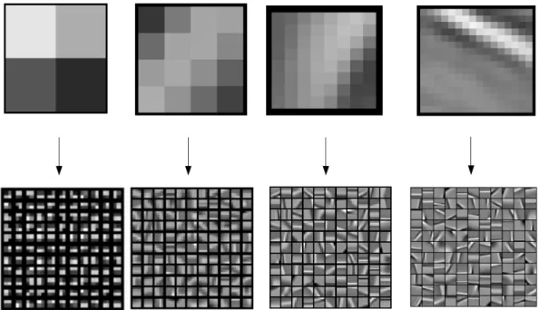
Figure 4. Top row from the left to the right 2x2 , 4x4, 8x8, 16x16 codewords corresponding to their respective bottom row 121 codewords dictionaries

2.4. Feature coding

With the dictionary and feature vectors in hand, we can obtain the coding matrix which generally describes the relationship between the feature vectors and the codewords (dictionary), where each feature vector activates a number of codewords thus forming a coding vector either with binary (hard vector quantization) or continuous elements (soft vector quantization, sparse coding) [51]. In our setup we use [51] call reconstruction based coding using a part of the codewords to describe the features via solving a least-square optimization problem, here theLasso(2), in fact both the dictionary and the coding matrix are obtained during the optimization step.

2.5. Feature pooling

The coding vectors obtained previously, are pooled over the whole image to form one pooling vector who is the final representation of the input image. Between the two popular pooling strategies used in the literature namely max pooling and average pooling, it has been shown [17] that max pooling is superior. Given α= [α1, ..., αn]∈Rk∗nthe coding matrix andi= [1, ..., N]∈ Nmthe indice of feature location per image

m= 1, ..., M, we obtain the following max pooled vector: zm,j = max

i∈N αi,j,for j=1,...,k,(3) wherezm∈Rkis the vector representing the whole imagem.

3. ONLINE DICTIONARY LEARNING

The algorithm described in this section in algorithm 1 is assuming a training set composed of independent and identically distributed samples and alternates at each loop between computing the decompositionαtof the training samplext over the dictionaryDt−1 obtained during the previous iteration and updating the dictionaryDtby minimizing the function:

Algorithm 1Online dictionary learning.

Precondition: x∈Rmp(x)(random variable and an algorithm to draw i.i.d sample ofp),λ∈R(regularization parameter),D0∈Rmxk(initial dictionary),T(number of iterations)

1: A0←0 .(reset the ”past” information)

2: B0←0

3: fort←1toT do 4: Drawxtfromp(x)

5: Sparse coding: compute using LARS

αt= argmin α∈Rk

1

2||x−Dt−1α||

2

2+λ||α||1.(4)

6: At←At−1+αtαTt

7: Bt←Bt−1+xtαTt

8: ComputeDtusing Algorithm 2, withDt−1as warm restart, so that

Dt= argmin D

1

t t X

i=1

1

2||xi−Dαi||

2

2+λ||αi||1.(5) = argmin

D 1

t(

1 2T r(D

T_DA

t)−T r(DTBt)).

9: end for

10: returnDT (learned dictionary)

3.1. Sparse coding

The sparse coding problem in (2) with fixed dictionary is an l1-regularized linear least-squares problem. In the case of dictionary columns with low correlation, simple methods based on coordinate descent with soft thresholding [52, 53] are enough. But the columns of the dictionary are more often than not highly correlated, and it is proved that a Cholesky-based implementation Lars algorithm [54, 55] that provides the entire regularization path can be as fast as simpler soft thresholding based methods while having a higher accuracy.

Algorithm 2Dictionary Update.

Precondition: D= [d1, ..., dk]∈Rmxk(input dictionary) 1: repeat

2: forj←1tokdo

3: Update the j-th column to optimize for (6) 4: uj← _A1_jj(bj−Daj) +dj

5: dj←_max(||1_uj||2,1)uj

6: end for 7: untilconvergence

8: returnD(updated dictionary) 3.2. Dictionary update

The dictionary update algorithm uses block coordinate descent with warm restarts, does not require any learning rate tuning and is parameter-free and since the vectors are sparse, the coefficients of A are diagonaly concentrated the block coordinate descent more efficient. In practice, Algorithm 2 updates each j-th column of D sequentially and (6) gives the solution of the dictionary update with respect to the j-th column, while keeping the other ones fixed under the constraintdT

jdj ≤ 1. It has been shown that this

optimization problem converges to a global optimum [56]. This algorithm uses a warm restart but other approaches have been proposed to update D, for instance, [57] suggest using a Newton method on the dual of (5).

4. THE VEHICLE LICENSE PLATE LOCATION ALGORITHM 4.1. Horizontal gradient

It is known that the most discriminative part of a vehicle, mainly its front and its rear are composed of horizontal lines [58], while the license plate region has a predominance of vertical lines. We apply the Sobel operator to obtain the vertical lines [59]. Figure 5(b) shows the resulting image of horizontal gradient detection on the original image in Figure 5(a). And to have a clearer emphasis on the license plate region, due to the great concentration of high valued pixels, we apply a mean filter [60] to the image. The final stage of the horizontal gradient phase can be seen in Figure 5(c).

4.2. Filtering

The goal of this phase is to darken every non license plate region. Morphological operations proposed in [61, 62] are applied to the image to darken high valued regions that don’t fit the expected size. Small non-VLP salient regions are darkened by a morphological opening operation as shown in Figure 5(d). The joint application of mean filter and opening operation causes undesirable variation among pixel values of license plate region though, perceived as gaps between its vertical saliences. We restore smoothness in these values which is equivalent to replenish the artificial created gaps using a morphological closing operation. Big non license plate regions are also darkened by a top-hap filtering,so that big salient regions will have their pixel’s values lowered as shown in Figure 5(e). As a result the license plate region may exibit unwanted artifacts in that the space between the letters and the numbers may be less salient. And the binarization process may therefore perform poorly splitting the license plate region into multiple parts, that problem can be fixed by applying a closing operation on the image. We then remove the saliences in the licence plate’s borders that may appear during the horizontal gradient step to find the tightest boundary of the license plates characters. We finally close the filtering phaseby applying an erosion operation followed by a dilation operation.

4.3. Adjustement

The adjustement phase generates potential license plate regions in a binary image. The first step is to binarize the image to separate salient regions from the background using Otsu’s method [63] to automatically define the binarization threshold and minimize the chance of a miss as depicted in Figure 5(g). A problem that could arise is that it is possible that the contrast between dark non license plate regions and the brighter license plate region is not big enough and could result in a ”botched” binarization. In the connected component

analysis we remove any region that is not license plate shaped from the binary image and finally we maintain only the license plate region candidates bounding boxes. We also eliminate candidates that are intercepting each other because the license plate region is essentially composed of vertical edges that do not intercept each other. Other vertical edge dominant candidates like signs that contant letters are not close enough to their regions intercept on the other hand candidates originated from background noise have a greater chance to touch each other given their random location. For the remaining candidates, we first cut the initial corresponding bounding box off of the monochrome image of the filtering phase like shown in Figure 5(f) and consider it as a separate candidate image. Second, a new binarization takes place with Otsu’s method and the candidate’s boundary is expanded to include lower valued pixels by a dilation operation. The resulting binary image may still contain undesired regions, which are erased by an erosion operation followed by a dilation. Finally, the resulting candidate bounding box is checked to see if minimum dimension constraints are satisfied if not, the candidate is discarded unless it is the last one, in which case it is kept. If there is no candidate or all of them are discarded, a histogram equalization is performed in the original image, to get a contrast improvement, and the location process is repeated from its very beginning.

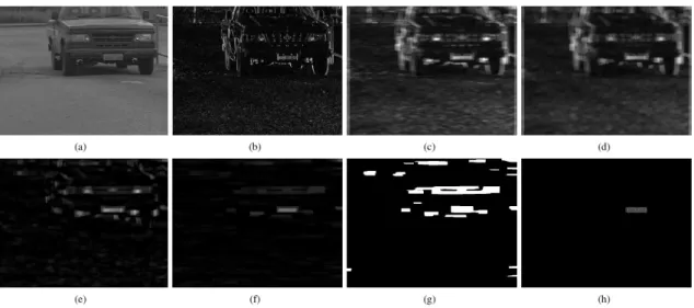
Figure 5. Steps of the vehicle license plate location method: (a) Original image, (b) Horizontal gradient, (c) Mean filter on horizontal gradient, (d) Small saliences darkened, (e) Big saliences darkened, (f) Erosion

and dilation operations, (g) Binarization, (h) Finding the vehicle license plate

5. CLASSIFICATION METHODS

5.1. Multi-class support vector machines

Multi-class classification is achieved here by using a ”one against one” scheme with probability estimates [64–66] thus training for k classes k(k-1)/2 classifiers, one for each pair of classes. Given k classes, estimate the pairwise class probabilities:

ri,j≈P(y=i|y=jori, x)≈ 1

1 +eAf+B,(7)

wheref is the decision value atxand A, B are estimated by minimizing the log likelihood of training data. With all theri,jwe can obtain thepiby optimizing the following objective function:

min p

1 2

k X

i=1

X

j:j6=i

(ri,jpi−rj,ipj)2,(8)

subject topi≥0,∀i, k X

i=1 pi= 1

for anyxwe assign it to the class of its highestpi.

5.2. Supervised K-means

The k-means [67] algorithm is one the simplest clustering algorithms which given a set of data x aims to separate it into k different clusters by optimizing the following objective function:

min c

k X

i=1

n X

j=1

||xj−ci||22,(9)

whereciis the cluster center. The standard implementation uses Lloyd’s algorithm [68] which consists of the

following two steps:

(a) Initial step: where the centroids are initialized.

(b) Assignment step: where each data point is assigned to a specific cluster based on its distance with the cluster’s cent

(c) Update step: where we compute the new centroids for each cluster.

In our implementation, we skip the update step so the centroids are initialized once, using only the training data. Then each test point is assigned to a specific cluster using its Euclidian distance to the respective centroid.

6. EXPERIMENTAL RESULTS

Using the COMVis car dataset [7] we build our set by clipping automatically from each image the most discriminative region of interest for make and model recognition, the front part of the car using [35] algorithm for license plate detection. In our experiment we usefive car makes, Suzuki, Toyota, Mitsubishi, Hyundai and Honda with respectively 153, 78, 36, 37 and 97 images. Note that these images contain different models, 8 for Suzuki, 4 for Toyota, 2 for Mitsubishi and Hyundai and 5 for Honda, thus increasing the overall difficulty of the recognition task due to unbalanced datasets. We build our feature matrix by concatenating the feature vectors (2x2, 4x4, 8x8, 16x16 blocks) of each image and then optimize theLasso(2) using [49] and the least angle regression [69] (LARS) algorithms to obtain the dictionary and the coding matrix. The pooling strategy (3) applied to the coding matrix gives us a representing vector for each image. These vectors are then fed to a linear kernel support vector machine (SVM) via a cross-validation framework holding out 80% as training data, this process is repeated one hundred times to obtain the recognition rates of Tables 1 and 2. The results here are obtained using the square mapped gradient descriptor (1) applied to a 128x512 image thus obtaining 128x1024 resulting matrix, which is a concatenation of the image under the SMG descriptor along direction x and the image under the SMG descriptor along y. This new image is considered the input of the feature matrix generation step. In Table 2, we use supervised k-means instead of the SVM classifier which achieves similar performance as the use of SMG+SVM setup without dictionary learning with an accuracy of 85.01±2.68, compared to 80.66±2.78 for the SMG+KMeans setup without dictionary learning.

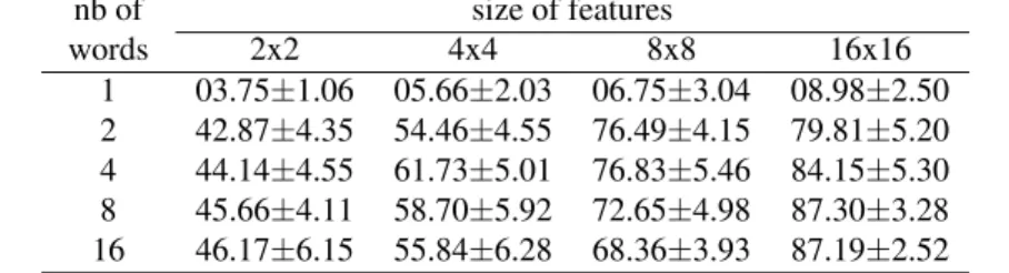
Table 1. Accuracy of the Kmeans+SMG setup different dictionary and feature vector sizes. nb of

words

size of features

2x2 4x4 8x8 16x16

1 03.75±1.06 05.66±2.03 06.75±3.04 08.98±2.50 2 42.87±4.35 54.46±4.55 76.49±4.15 79.81±5.20 4 44.14±4.55 61.73±5.01 76.83±5.46 84.15±5.30 8 45.66±4.11 58.70±5.92 72.65±4.98 87.30±3.28 16 46.17±6.15 55.84±6.28 68.36±3.93 87.19±2.52

Table 2. Accuracy of the SVM+SMG setup for different dictionary and feature vector sizes. nb of

words

size of features

2x2 4x4 8x8 16x16

1 03.45±2.06 04.23±1.28 04.18±2.50 08.64±2.54 2 46.46±5.83 60.81±5.45 78.60±4.59 84.38±4.46 4 48.07±4.50 66.42±4.51 80.09±4.59 86.38±3.53 8 50.76±5.17 65.62±4.82 77.52±4.77 89.82±3.27 16 51.03±5.09 65.56±4.86 75.40±3.23 89.99±2.45

7. CONCLUSION

Despite an amelioration of performance the optimization cost can be quite heavy especially in an online framework. Rigamonti et al [70], showed that enforcing sparsity is not helpful for recognition rates when extracting the features and that the same performance can be achieved through the use of plain convolution, however sparsity is still important when learning the filters. They did use a different equation than (2), where the matrix-vector product is replaced by a convolution and a two step algorithm where learning the filters and extracting the features are separated. The problem remains that sparsity do not dramatically increase performance nor is it required to obtain good results. Even then and to put sparsity in perspective, it must be inserted in a bigger framework like in hierarchical models, deep belief networks (DBNs) [71] to show its usefulness.

REFERENCES

[1] V.S. Petrovic and T.F. Cootes,Analysis of Features for Rigid Vehicle Type Recognition. British Machine Vision Conference, 2004.

[2] I. Zafar, E.A. Edirisinghe, S. Acar and H.E. Bez, Two Dimensional Statistical Linear Discriminant Analysis for Real-Time Robust Vehicle Type Recognition. Proc. SPIE 6496, Real-Time Image Processing, 2007.

[3] X. Clady, P. Negri, M. Milgram and R. Poulenard,Vehicle make and model identification using vision sytem. Traitement du signal, 2009.

[4] A. Psyllos, C.N. Anagnostopoulos and E. Kayafas,Vehicle Authentification from Digital Image Measure-ments. 16th IMEKO TC4 Symposium, 2009.

[5] S. Badura and S. Foltan,Advanced scale-space, invariant, low detailed feature recognition from images-car brand recognition. Proceedings of the International Multiconference on Computer Science and Incromation Technology, 2010.

[6] G. Pearce and N. Pears,Automatic Make and Model Recognition from Frontal Images of Cars. 8th IEEE International Conference on Advanced Video and Signal-Based Surveillance, 2011.

[7] M.S. Sarfraz and M.H. Khan, A Probabilistic Framework for Patch Based Vehicle Type Recognition. International Conference on Computer Vision Theory and Applications, 2011.

[8] B. Zhang and Y. Zhou,Vehicle Type and Make Recognition by Combined Features and Rotation Forest Ensemble. International Journal of Pattern Recognition and Artificial Intelligence, 2012.

[9] B. Daya, A. Akoum and S. Bahlak,Geometrical Features for Multiclass Vehicle Type Recognition using MLP Network. Journal of Theoretical and Applied Information Technology, 2012.

[10] H. Yang, L. Zhai, L. Li, Z. Liu, Y. Luo, Y. Wang, H. Lai and M. Guan, An Efficient Vehicle Model Recognition Method. Journal of Software, 2013.

[11] V. Varjas and A. Tanacs,Car Recognition from Frontal Images in Mobile Environment. 8th International Symposium on Image And Signal Processing and Analysis, 2013.

[12] D.M. Jang and M. Turk,Car-Rec: A Real Time Car Recognition System. IEEE Workshop on Applications of Computer Vision, 2011.

[13] F.M. Kazemi, S. Samadi, H. Pourreza and M.R. Akbarzadeh, Vehicle Recognition Based on Fourier, Wavelet and Curvelet Transforms- a Comparative Study. International Journal of Computer Science and Network Security, 2007.

[14] M. AbdelMaseeh, I. Badreldin, M.F. Abdelkader and M. El Saban, Car Make and Model recognition combining global and local cues. 21st International Conference on Pattern Recognition, 2012.

[15] A. Psyllos, C.N. Anagnostopoulos and E. Kayafas, Vehicle Logo Recognition Using a SIFT-Based Enhanced MAtching Scheme. IEEE Transactions on Intelligent Transportation Systems, 2010.

[16] J. Prokaj, and G. Medioni, 3-D Model Based Vehicle Recognition. Workshop on Applications of Computer Vision, 2009.

[17] Y.L. Bourreau, F. Bach, Y. LeCun and J. Ponce, Learning Mid-Level Features for Recognition. Conference on Computer Vision and Pattern Recognition, 2010.

[18] G.E. Hinton and R.R. Salakhutdinov, Reducing the Dimensionality of Data with Neural Networks. Science, 2006.

[20] A. Olshausen and D. J. Field,Emergence of simple-cell receptive field properties by learning a sparse code for natural images. Nature, 381:607–609, 1996.

[21] B. A. Olshausen and D. J. Field,Sparse coding with an overcomplete basisset: A strategy employed by V1?. Vision Research, 37(23):3311–3325, 1997

[22] R. Raina, A. Battle, H. Lee, B. Packer, and A. Y. Ng, Self-taught learning: transfer learning from unlabeled data. In Proceedings of the International Conference on Machine Learning (ICML), 2007 [23] J. Yang, K. Yu, Y. Gong, and T. Huang,Linear spatial pyramid matching using sparse coding for image

classification. In Proceedings of the IEEE Conference on Computer Vision and Pattern Recognition (CVPR), 2009.

[24] M. D. Zeiler, G. W. Taylor, and R. Fergus, Adaptive deconvolutional networks for mid and high level feature learning. In Proceedings of the International Conference on Computer Vision (ICCV), 2011. [25] A. Rakotomamonjy, Direct optimization of the dictionary learning problem. IEEE Transactions on

Signal Processing, vol. 61, no. 22, pp.5495–5506, Nov 2013.

[26] N. M. Nasrabadi and R. A. King,Image coding using vector quantization: A review. IEEE Transactions on Communications, 36(8):957–971, 1988.

[27] A. Gersho and R. M. Gray,Vector quantization and signal compression. Kluwer Academic Publishers, 1992.

[28] P. Paatero and U. Tapper, Positive matrix factorization: a non-negative factor model with optimal utiliza-tion of error estimates of data values. Environmetrics, 5(2):111–126, 1994.

[29] D. D. Lee and H. S. Seung,Learning the parts of objects by non-negative matrix factorization. Nature, 401(6755):788–791, 1999.

[30] A. Cutler and L. Breiman,Archetypal analysis. Technometrics, 36(4):338–347, 1994.

[31] J. H´erault, C. Jutten and B. Ans, D´etection de grandeurs primitives dans un message composite par une architecture de calcul neuromim´etique en apprentissage non supervis´e. Actes du X`eme Colloque GRETSI, 1985.

[32] A. J. Bell and T. J. Sejnowski, An information-maximization approach to blind separation and blind deconvolution. Neural computation, 7(6):1129–1159, 1995.

[33] A. J. Bell and T. J. Sejnowski, The “independent components” of natural scenes are edge filters. Vision Research, 37(23):3327–3338, 1997.

[34] A. Hyv¨arinen, J. Karhunen and E. Oja, Independent component analysis. John Wiley and Sons, 2004. [35] P.R. Mendes J`unior, J.M.R. Neves, A.I. Tavares and D. Menotti,Towards an automatic vehicle access

control system: license plate location. In Proceedings of international conference. Systems, Man and Cybernetics, 2011.

[36] M. Marszalek, C. Schmid, H. Harzallah and J. Van de Weijer,Learning Representations for Visual Object Class Recognition. ICCV Workshop on the PASCAL VOC Challenge, 2007.

[37] N. Dalal and B. Triggs,Histograms of Oriented Gradients for Human Detection. Conference on Com-puter Vision and Pattern Recognition, 2005.

[38] C. Harris and M. Stephens,A Combined Corner and Edge Detector. The Fourth Alvey Vision Confer-ence, 1988.

[39] D.G. Lowe,Distinctive Image Features from Scale-Invariant Keypoints. International Journal of Com-puter Vision, 2004.

[40] H. Bay,A. Ess,T. Tuytelaars and L. Van Gool,Speeded-Up Robust Features(SURF). European Confer-ence on Computer Vision, 2006.

[41] E. Nowak, F. Jurie and B. Triggs, Sampling Strategies for Bag-of-Features Image Classification. 9th European Conference on Computer Vision, 2006.

[42] T. Lindeberg,Detecting Salient Blob-Like Image Structures and Their Scales with a Scale-Space Primal Sketch: A Method for Focus-of-Attention. International Journal of Computer Vision, 1993.

[43] P.N. Belhumeur, J.P. Hespanha and D.J. Kriegman,Eigenfaces vs. Fisherfaces: Recognition Using Class Specific Linear Projection. IEEE Transactions on Pattern Analysis and Machine Intelligence, 1997. [44] A.A. Martinez and A.C. Kak,PCA versus LDA. IEEE Transactions on Pattern Analysis and Machine

Intelligence, 2001.

[45] K. Etemad and R. Chellappa,Discriminant Analysis for Recognition of Human Face Images. Journal of the Optical Society of America, 1997.

[46] S. Lazebnik, C. Schmid and J. Ponce,Beyond bags of features: Spatial matching for recognizing natural scene categories. Conference on Computer Vision and Pattern Recognition, 2006.

[47] J. Yang, K. Yu, Y. Gong and T. Huang,Linear Spatial Pyramid Matching using Sparse Coding for Image Classification. Conference on Computer Vision and Pattern Recognition, 2009.

[48] J. Mairal, F. Bach,J. Ponce,G. Sapiro and A. Zisserman,Supervised Dictionary Learning. Advances in Neural Information Processing Systems, 2008.

[49] J. Mairal, F Bach, J. Ponce and G. Sapiro,Online Learning for Matrix Factorization and Sparse Coding. Journal of Machine Learning Research, 2010.

[50] R. Tibshirani,Regression Shrinkage and selection via the Lasso. Journal of the Royal Statistical Society Series, 1996.

[51] Y. Huang, Z. Wu, L. Wang and T. Tan,Feature Coding in Image Classification: A Comprehensive Study. IEEE Transactions on Pattern Analysis and Machine Intelligence, 2013.

[52] W. Fu, Penalized Regressions: The Bridge Versus the Lasso. Journal of computational and graphical statistics, 1998.

[53] J. Friedman, T. Hastie, H. Holfling and R. Tibshirani, Pathwise coordinate optimization. Annals of Statistics, 2007.

[54] M. Osborne, B. Presnell and B. Turlach,A new approach to variable selection in least squares problems. IMA Journal of Numerical Analysis, 2000.

[55] B. Efron, T. Hastie, I. Johnstone and R. Tibshirani,Least angle regression. Annals of Statistics, 2004. [56] D. Bertsekas,Nonlinear programming. Athena Scientific Belmont, 1999.

[57] H. Lee, A. Battle, R. Raina and A.Y. Ng, Efficient sparse coding algorithms. Advances in Neural Information Processing Systems, 2007.

[58] M. Sarfraz, M.J. Ahmed and S.A. Ghazi,Saudi arabian license plate recognition system. In Proceedings of the International Conference on Geometric Modeling and Graphics (GMAG), 2003.

[59] B. Hongliang and L. Woods,Digital Image Processing. 3rd ed. Prentice Hall, 2007.

[60] R.C. Gonzalez and L. Changping,A hybrid license plate extraction method based on edge statistics and morphology. In Proceedings of the International Conference on Pattern Recognition (ICPR), 2004. [61] F. Martin, M. Garcia and J.L. Alba, New methods for automatic reading of VLP’s (Vehicle License

Plates). In Proceedings of IASTED International Conference on Signal Processing, Pattern Recognition, and Applications (SPPRA), 2002.

[62] P.V. Suryanarayana, S.K. Mitra, A. Banerjee and A.K. Roy,A morphology based approach for car license plate extraction. In Proceedings of the IEEE INDICON, 2005.

[63] N. Otsu,A threshold selection method from gray-level histograms. IEEE Transactions on Systems, Man, and Cybernetics (SMC), 1979.

[64] U.H.G. Kressel, Pairwise classification and support vector machines. Advances in Kernel Methods, 1998.

[65] T.F. Wu, C.J. Lin and R.C. Weng,Probability estimates for multi-class classification by pairwise coupling. Journal of Machine Learning, 2004.

[66] H.T. Lin, C.J. Lin and R.C. Weng,A note on Platt’s probabilistic outputs for support vector machines. Machine Learning, 2007.

[67] J.B. MacQueen,“Some Methods for classification and Analysis of Multivariate Observations. Proceeed-ings of 5th Berkeley Symposium on Mathematical Statistics and Probability, 1997.

[68] P.S. Lloyd,Least Square Quantization in PCM. IEEE Transactions on Information Theory, 1982. [69] B. Efron,T. Hastie, I. Johnstone and R. Tibshirani,Least Angle Regression. The Annals of Statistics,

2004.

[70] R. Rigamonti, M.A. Brown and V. Lepetit,Are Sparse Representations Really Relevant for Image Classi-fication?. IEEE Conference on Computer Vision and Pattern Recognition, 2011.

[71] H. Lee, R. Grosse, R. Ranganath and A.Y. Ng,Convolutional deep belief networks for scalable unsuper-vised learning of hierarchical representations. International Conference on Machine Learning, 2009.