Labor Leverage and the Value Premium
∗A. DONANGELO, F. GOURIO, and M. PALACIOS†
ABSTRACT
We show that labor leverage, proxied by labor share, explains roughly half of the value premium but not future cash flow growth. The other half of the value premium is determined by the component of the book-to-market ratio that is orthogonal to labor share, and this component explains most of future cash flow growth. To explain these findings, we propose a parsimonious labor-based production model for firms. Our results suggest that the defining aspect of a growth firm is not a low book-to-market ratio, but rather a small component of book-to-market ratio that is not explained by labor share.
∗This version: September 2015.
†Donangelo is with the Finance Department at the University of Texas at Austin. Gourio is with the
Firms with high book-to-market ratios tend to have higher average returns than those with
low ratios, a regularity known as the value premium. After decades of research, the literature
still has not reached a consensus on a micro-founded explanation for this regularity. A
possible reason for this lack of convergence is that most of the literature has been searching for
asingle economic mechanism to explain the value premium. We present evidence that labor-induced operating leverage, which we denote by the term labor leverage, is a fundamental part of the explanation. In particular, we find that labor leverage explains approximately
50% of the value premium. But, notably, this paper shows that labor leverage complements
at least one fundamentally different growth-based mechanism..
Labor leverage is a promising candidate mechanism to explain the value premium for
two reasons. The first reason is that labor compensation represents the most significant cost
for the average firm.1 The second reason is that labor leverage is arguably intrinsically less endogenous than other forms of leverage, such as financial leverage.2 In fact, as documented in Donangelo et al. (2015), labor share (i.e., the ratio of labor costs to value added), which
proxies for labor leverage, is significantly positively related to asset returns.
A firm’s high book-to-market ratio can be explained by two factors: high discount rates
required by investors or low expected earnings growth relative of those of a low
book-to-market ratio firm.3 To quantify the relative weights of these two factors, Cohen, Polk, and Vuolteenaho (CPV, 2003) propose a methodology to decompose the cross-sectional variation
1The significance of labor costs is well documented in Gollin (2002), for example, who finds that the
share of labor expenses in GDP is between 0.65 and 0.80 across developed countries.
2See, for example, Lin and Favilukis (2014) for a discussion of labor cost rigidity. Also, Donangelo,
Gourio, and Palacios (2015) document that labor costs are significantly less variable than other costs: In our sample, a 1% reduction in sales leads, on average, to a 0.62% reduction in staff expenses but a 1.23% reduction in all other costs.
3As argued by Berk (1995), the cross-sectional variation in book-to-market ratios must be partially
of book-to-market ratios into components related to discount rates and growth rates.4 Note that the component of the cross-sectional variation in book-to-market ratios related
to future discount rates is the value premium. We build upon this insight and extend the methodology in CPV to quantify the weight of contemporaneous labor share in explaining the
value premium. In particular, we pre-decompose book-to-market ratios into two components:
One component is explained by labor share and the other is orthogonal to labor share.
We denote these components by bm‖S and bm⊥S, respectively. The fact that these two
components are orthogonal implies that book-to-market ratio is equal to the sum of the
contribution of the component of book-to-market ratio variation that is related to future
returns. We show that the projection of labor share on book-to-market ratio (i.e., bm‖S)
explains approximately 50% of the cross-sectional variation of book-to-market ratios related
to variation in future returns. In addition to the variance decomposition methodology, we also
employ standard panel data regressions and portfolio sorts that employ the two components
of the book-to-market ratio. These findings confirm the economic significance of labor share
in explaining the value premium.
It is plausible that labor leverage explains not only cross-sectional differences in expected
returns but also differences in cash flow growth rates.5 Our extended variance decomposition methodology also allows us to investigate the explanatory power of labor share on the
com-ponent of book-to-market ratios related to future earnings growth. Notably, when compared
to bm⊥S, bm‖S explains relatively less of the relation between the cross-sectional variation
in book-to-market ratio that is related to variation in future earnings growth. We
inter-pret this finding as evidence for a fundamental difference in the labor leverage mechanism,
4In practice, the methodology also decomposes cross-sectional variation of book-to-market ratios into a
third residual component, because the use of a finite sample of real data forces the methodology to use a relatively short forward-looking horizon of 1 to 10 years. As discussed in CPV, the residual picks up the persistence of book-to-market ratios. In other words, a firm’s high book-to-market ratio today is partially explained by an expected high book-to-market ratio in 10 years, which in turn is likely to be explained by high future discount rates or high future growth rates.
5For instance, labor leverage is negatively related to productivity, as shown in Donangelo et al. (2015);
which is captured by bm‖S, and mechanisms unrelated to labor share, which are captured
by bm⊥S
. In particular, we find that bm⊥S
explains most of component of the variation
in book-to-market ratios related to differences in earnings growth. We confirm this finding
by showing that bm⊥S
has greater time-series predictive power for sales and asset growth
at various horizons, ranging from 1 to 10 years. The results presented suggest that it is
unlikely that a single growth-based mechanism (i.e., a mechanism driven by investment or
distress) can explain the value premium. Moreover, these results suggest that a low bm⊥S
is a better determinant of a growth firm than a low book-to-market ratio alone. In other words, our findings suggest that the defining aspect of a firm that is expected to experience
relatively high future growth (i.e., a growth firm) is not a low book-to-market ratio, but a low magnitude of the component of the book-to-market ratio that is unexplained by labor leverage.
To establish the link between labor leverage and the value premium, we propose a
production-based asset model of a firm that is exposed to perfect labor markets. The model
extends that in Donangelo et al. (2015) by incorporating cross-sectional heterogeneity in
fu-ture growth opportunities. These opportunities are represented in the model as firm-specific
shocks to earnings growth. These shocks are unrelated to contemporaneous labor share, and
they complement the labor leverage mechanism in explaining the cross-sections of expected
asset returns and book-to-market ratios. The model provides two new implications, both of
which are consistent with our empirical findings. The first implication is that labor share
is positively related to expected asset returns while not significantly correlated to future
growth rates. The second implication is that the component of book-to-market ratios not
explained by labor share is related to cross-sectional differences in expected future growth.
The theoretical approach of this paper relates to previous studies of the cross-section
of returns based on micro-level dynamic decisions.6 Our main departure point from the
6A very partial list of work from this literature is Berk, Green, and Naik (1999); Carlson, Fisher, and
literature is that, in our work, the mechanism is related to labor whereas most of this
literature is based on mechanisms related to installed capital or to changes thereof.7
A growing strand of the literature considers the role of labor for asset pricing in the
cross-section. But these papers tend to focus on alternative frictions or aggregate (time series)
facts. For instance, Belo, Lin, and Bazdresch (2014) explore adjustment costs in labor and
relate observable hiring and firing decisions to future investment opportunities, which in turn
affect expected returns. Lin and Favilukis (2014) demonstrate the effect of wage rigidity on
the aggregate stock market value.8
We contribute to another strand of the literature that discusses the relation between
labor leverage and asset prices. Donangelo (2014) proposes a model in which labor mobility
is positively related to labor leverage. Labor share and labor mobility are two complementary
mechanisms that affect a firm’s operating leverage. In a cyclical industry, the effect of labor
mobility on firm risk increases in labor share, and the effect of labor share on firm risk
increases in labor mobility. Danthine and Donaldson (2002) discuss a mechanism in which
countercyclical capital-to-labor share leads to labor leverage in a general equilibrium setting.
In their model, wages are less volatile than profits, due to the limited market participation of
workers; and firms insure workers against labor risk through labor contracts. Stable wages
act as an extra risk factor for shareholders, since markets are incomplete in their model.
Last, while our work focuses on the interaction between workers and firms in a spot labor
market, a growing body of literature explores the implications of implicit contracts for the
riskiness of wages and firms.9 Most recently, Zhang (2014) derives predictions similar to our model, based on the optimal implicit contract between workers and firms. Whereas our
7While not specifically related to labor, Imrohoroglu and Tuzel (2014), establish a link between
produc-tivity and profitability on stock returns. Any form of leverage, being financial or operating (labor-induced or “traditional”), is amplified when productivity is low. In this sense, our work micro-founds the productivity channel by providing support for the labor leverage mechanism.
8Other papers that relate labor and asset pricing are Kuehn, Petrosky-Nadeau, and Zhang (2013), ?,
Chen, Kacperczyk, and Ortiz-Molina (2012), Eisfeldt and Papanikolaou (2013), and Favilukis and Lin (2015).
9See, for instance, Harris and Holmstrom (1982), Berk, Stanton, and Zechner (2010), Parlour and Walden
dynamics stem from the interaction of events in the wider economy and the firm, this line
of the literature focuses on the interaction between a worker’s productivity, the firm, and
the economy-wide labor market. In reality, variations in the worker’s productivity as well as
changing conditions outside the firm affect its riskiness. In this sense, we consider our spot
labor market analysis as complementary to the implicit contracts analysis..
I. Empirical Evidence
In this section, we show the empirical link between labor share, book-to-market ratios,
and the value premium. We use the findings presented in this section to motivate the
production-based model in Section II with labor leverage and shocks to productivity growth
rates.
A. Data
We follow Donangelo et al. (2015) and construct two closely related empirical measures
of labor share. The first measure of labor share (hereafter LS) is defined as follows:
LS𝑖𝑡≡
XLR𝑖𝑡
OIBDP𝑖𝑡+XLR𝑖𝑡+INVFG𝑖𝑡−INVFG𝑖𝑡−1
, (1)
whereXLRis Compustat variable “Staff Expense – Total,” which we use as a proxy for labor costs; OIBDP is Compustat variable “Operating Income Before Depreciation”; and INVFG
is Compustat variable “Inventories –Finished Goods.”10 We include the change in inventories of final goods to make the empirical measure consistent with the theoretical measure because
some of the goods produced over a given year are not sold during that year. Likewise, a
10According to the U.S. GAAP definition,XLR is closely related to labor costs since it represents the
portion of the goods sold by the firm in a given year were produced in previous years.11 A limitation of the LS measure is that, since the variableXLRis a supplementary income statement item, it is only available for roughly 12% of firm-year observations in our sample.
To address this limitation, we use a second measure, which we denote as “extended” labor
share (hereafter ELS). We define ELS as follows:
ELS𝑖𝑡 ≡ ⎧ ⎨
⎩
LS𝑖𝑡 if XLR is non-missing
LABEX𝑖𝑡
OIBDP𝑖𝑡+LABEX𝑖𝑡+INVFG𝑖𝑡−INVFG𝑖𝑡−1 if XLR is missing,
(2)
whereLABEX is a constructed variable defined as the product of Compustat variableEMP
(“Number of Employees”) and the average annual labor compensation per employee in the
industry during that year.12 We exclude from our sample all firm-year observations in which ELS is negative or greater than one.
Table I reports time series averages of median characteristics for portfolios of firms sorted
on LS (Panel A) and ELS (Panel B). Novy-Marx (2011) presents evidence that intra- as
opposed to inter-industry differences in book-to-market ratios are more closely related to
cross-sectional variation in operating leverage intensity. For this reason, the statics are
presented in simple sorts and also in within-industry sorts. The second and third columns
of Panel A are identical, since ELS is defined as LS in the subsample of firms in which
the latter is non-missing. More telling is the fact that the second and third columns of
Panel B are quite similar as well. We interpret this fact as evidence that the distribution
of ELS conditional on missing LS is not significantly different from the distribution of ELS
conditional on non-missing LS. The fourth column reports that the number of employees per
unit of plant, property, and equipment (PPE) is increasing in both LS and ELS. This last
finding is consistent with a positive relation between labor share and labor intensity.
11The results presented in the paper are qualitatively unaffected by excluding the change in inventories
from the measure.
12We estimate the average labor compensation per employee as the average ratio ofXLR and EMP in
Columns 5 to 11 of the two panels show qualitatively similar trends in the statistics
across labor share quintiles. For instance, high labor share firms tend to have higher
book-to-market ratios than low labor share firms, in particular in industry-adjusted sorts. The
table also shows a negative relation between labor share and both market value of equity
and book value of assets. The negative trend in the market value of equity is consistent
with the hypothesized greater riskiness of high labor share firms. A possible explanation for
the negative trend in asset values is a downward bias in asset value reporting, in particular
since high labor share firms are both less capital intensive and have fewer tangible assets.13 Consistent with a reporting bias, the panels report that the value of organizational capital,
which is not considered in a firm’s financial reports, is increasing in labor share. Profitability
ratios and, to some extent, leverage ratios seem fairly unrelated to labor share.
<<
Table I here
>>
B. Decomposition of the Value Spread
The labor leverage mechanism amplifies not only idiosyncratic risk but also the exposure
to any source of systematic risk that affects the firm. Through its effect on systematic risk
loading amplification, labor leverage should also lead to higher discount rates and thus to
higher book-to-market ratios. In this sense, the relation between labor share and expected
asset returns must be fully subsumed by that of book-to-market ratios and expected asset
returns.14
13See Damodaran (2011) for a discussion of the relation between intangibles and a bias in asset value
reporting.
14Note that this argument does not imply the converse statement to be true. That is, the relation between
B.1. Labor Share and Book-to-Market Variance Decomposition
We start the presentation of our strategy to decompose book-to-market ratios by
revisit-ing a useful theoretical link between book-to-market ratios and expected returns. Consider
the log-linearized accounting identity described in Cohen, Polk, and Vuolteenaho (CPV,
2003). This identity relates the book-to-market ratio of a firm to its components related to
future discount rates and expected future earnings up to N periods ahead:
bm𝑡−1 = 𝑁 ∑︁
𝑗=0
𝜌𝑗𝑟𝑡+𝑗 + 𝑁 ∑︁
𝑗=0
𝜌𝑗(−𝑒𝑡+𝑗) +𝜌𝑁+1bm𝑡+𝑁, (3)
where all variables are expressed in logs and are demeaned, 𝑏𝑚 is log book-to-market ratio,
𝑟 is log gross asset return, 𝑒is log earnings, and 0< 𝜌 <1is a constant.15 The first term of the right-hand side of the equality represents the component of book-to-market ratio that is
attributed to higher future discount rates between years t and t+N. The second term is the
component attributed tolower earnings between years t and t+N. The last term represents the component attributed to discount rates and earning growth after year N. This last term
is related to the future book-to-market ratio prevailing at year N.
Decomposition (3) tells us that a high book-to-market ratio predicts either high future
asset returns (i.e., discount rates), low expected future earnings (i.e., cash flow) growth, or
a combination of the two. Labor share is closely related to discount rates and thus to the
term ∑︀𝑁𝑗=0𝜌𝑗𝑟
𝑡+𝑗. We argue that the relation between labor share andfuture discount rates
is analogous to that involving current discount rates from Equation (24) since labor share is
a persistent firm characteristic. A firm that has high labor share and risky cash flows today
is also expected to have a high labor share, and thus risky cash flows, for at least some time
in the future. Although related to the level of earnings, labor share is not directly related to earnings growth and therefore not related to the term ∑︀𝑁𝑗=0𝜌𝑗(−𝑒
𝑡+𝑗).
15The decomposition above is based on the assumption that earnings, dividends, and book values follow a
To analyze the relation between labor share and the components of the decomposition,
we extend CPV’s methodology and decompose the left-hand side variable in the identity
(3) into two orthogonal terms: one explained by labor share and the other orthogonal to
labor share. This extra decomposition is implemented through cross-sectional regressions of
book-to-market ratios on contemporaneous labor shares as shown below:
bm𝑖,𝑡 =𝛽0+𝛽S,tsharei,t+𝜖𝑖,𝑡, (4)
where 𝑠ℎ𝑎𝑟𝑒 denotes demeaned log labor share. We denote the component of log
book-to-market ratio predicted by labor share as bm‖S
and denote the component orthogonal to log
labor share as bm⊥S.16 These components are given by
bm‖S
𝑖,𝑡 ≡𝛽^S,tsharei,t, and (5)
bm⊥S
𝑖,𝑡 ≡bm𝑖,𝑡−𝛽^S,tsharei,t. (6)
The sum of the variances of bm‖S and bm⊥S equals the variance of book-to-market ratios.17 We use this fact to attribute the relative weights of bm‖S
and bm⊥S
in explaining the right
hand side terms of decomposition (3).
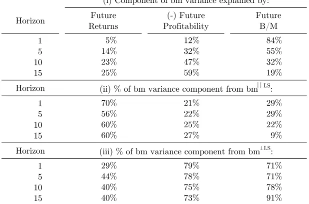
Panels A and B of Table II show the results from the decomposition using LS and ELS,
respectively, as proxies for labor share. The top rows of Panels A and B present the results
of the original decomposition from CPV applied to samples of firms with non-missing LS and
ELS, respectively. Although both of our working samples are smaller and cover different time
periods, we obtain results consistent with those in CPV. In particular, we also find that the
component related to future profitability dominates the component related to future asset
returns in explaining book-to-market ratios at longer horizons. The first column of the first
16The superscripts𝑆 represent either LS or ELS.
17In the sample with non-missing LS observations, we find that the variances of bm, bm‖S, and bm⊥S
group of rows shows that, at 15–year horizons, 35.7% (Panel A) and 36.0% (Panel B) of the
cross-sectional variation in book-to-market ratios is due to variation in future asset returns.
The second column shows that at similar horizons, 47.7% (Panel A) and 46.0% (Panel B) of
the cross-sectional variation in book-to-market ratios is due to variation in earnings growth.
The third column shows that the residual portion of variation in book-to-market ratios that
is unexplained by variation in either asset returns or earnings growth is 17.9% (Panels A and
B).
In Panels A and B, the first column of the second and third groups of rows presents the
first set of results from our extended decomposition. The sample sizes are quite different
across these two panels and are consistent with those in Panels A and B from Table I. The
first column of these rows shows the cross-sectional percentage variation of book-to-market
ratios related to future returns that is attributable to bm‖S and bm⊥S. Out of the variation
attributable to future returns, the portion attributable to bm‖S is 19.5% (approximately
55% of the total variation) and 20.4% (approximately 57% of the total). The equivalent
estimates for the portion attributable to bm⊥S are 16.3% (approximately 46% of the total)
and 15.6% (approximately 43% of the total). This last result is consistent with the idea
that alternative mechanisms, unrelated to current labor share, can partially explain future
discount rates. These findings highlight the importance of labor share in explaining the
value premium. Even when we consider different time horizons, bm‖S
consistently explains
a significant portion of the cross-sectional book-to-market ratio variation due to future asset
returns.
The second column of the second and third groups of rows in Panels A and B present the
second set of results from our extended decomposition. The second column of these rows
shows the cross-sectional percentage variation of book-to-market ratios related to future
profitability that is attributable to bm‖S and bm⊥S. Out of the variation attributable to
future profitability, the portion attributable to bm‖S
is 7.1% (approximately 15% of the
attributable to bm⊥S are 40.6% (approximately 85% of the total) and 40.4% (approximately
88% of the total). These results suggest that while both bm‖S
and bm⊥S
are related to
discount rates, bm⊥S is the component of book-to-market ratios more closely related to
future earnings growth. Given that earnings growth has a minus sign in (3), the result
indicates that earnings in high-bm⊥S firms are expected to have lower levels of growth than
earnings in low-bm⊥S firms. Low-bm⊥S–not simply low book-to-market ratio–seems to be
the defining characteristic of a growth firm.
In Panels A and B, the third column of the second and third groups of rows presents
the decomposition of the residual of the cross-sectional variation in future book-to-market ratios not explained by future returns or by future earnings. The residual is captured by the
book-to-market ratio at the end of the period considered. As discussed in CPV, this residual
is most likely related to future returns or to future earnings from that period onwards. The
finding that bm‖S explains less of the residual, for longer periods in particular, while the
opposite is true for bm⊥S
, also suggests a fundamental difference in the duration of the
information predicted by these components.
Taken as a whole, the findings in Table II indicate that two fundamentally different
mechanisms relate to the value premium. One, related to labor share, seems to explain
roughly 50% of the value premium, but is not significantly related to future growth. The
other mechanism, which is orthogonal to labor share, seems to be closely related to
growth-based or investment-growth-based stories, and it explains the remaining 50% of the value premium.
<<
Table II here
>>
C. Expected Asset Returns
In this section, we explore the empirical relation between expected returns and the
share. To address the challenge that expected returns are not observable, we use two
differ-ent types of proxies for them: realized stock returns and stock return loadings on risk factors
(i.e., betas).
C.1. Realized Asset Returns
The variance decomposition of book-to-market ratios in the last section suggests that
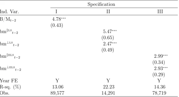
labor share partially explains the return spread between value and growth firms. Table III
provides additional supporting evidence for this finding. This table reports results of panel
data regressions of annual returns on book-to-market ratios as well as their components,
both explained (bm‖S) and unexplained (bm⊥S) by labor share. All independent variables
are standardized so that they have a mean of 0 and a standard deviation of 1. This
stan-dardization allows for a more direct comparison of the estimated coefficients from different
specifications. A one-standard-deviation cross-sectional increase in LS and ELS leads to
an increase in annual returns of 1.18% and 0.80%, respectively. A one-standard-deviation
cross-sectional increase in the projections of LS and ELS on book-to-market ratios leads to
increases in annual returns of 5.47% and 2.99%, respectively. The equivalent annual return
increase of a one-standard-deviation cross-sectional increase in the components of
book-to-market ratios orthogonal to LS and ELS are 2.47% and 2.93%, respectively. Taken together,
these results support the economic significance of the relation between labor share and priced
firm risk.
<<
Table III here
>>
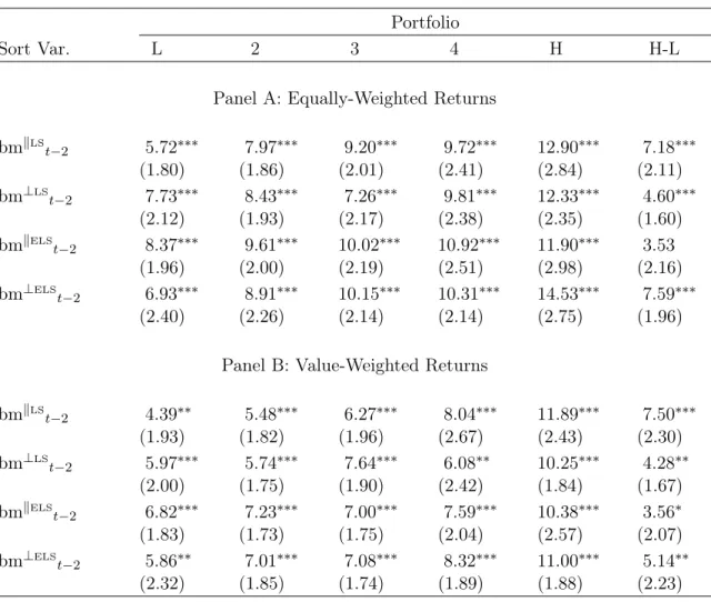
Table V presents average post-ranking two-years-ahead annual equity returns of quintiles
of stocks sorted on book-to-market ratios as well as bm⊥S and bm‖S. The last column shows
the returns of a portfolio that is long stocks in the highest quintile and is short stocks in
the lowest quintile (H-L portfolio). Portfolios are equally-weighted in Panel A and
that are comparable to those of firms with high bm⊥LS and bm⊥ELS, especially when LS is
used as a proxy for labor share. The return spread of the H-L portfolio formed with the
projections of labor share on book-to-market ratios is larger than that of the direct measures
found in Donangelo et al. (2015). This is not surprising, given that the measures of labor
share are likely subject to greater measurement error than the book-to-market ratio. If the
measurement error is unrelated to firm risk and cash-flow growth, it will be filtered out in
the projection.
<<
Table IV here
>>
C.2. Risk Factor Loadings
Under a rational expectation and in a full information setting, realized asset returns are
an unbiased, albeit noisy, proxy for unobservable expected asset returns.18 In this section, we use loadings on traditional risk factors (i.e., risk factor betas) as an alternative proxy for
expected asset returns. Note, however, that the use of empirical estimates of risk factor betas
as proxies for expected returns does not imply that this paper takes a stand on whether the
empirical implementations of the CAPM or other traditional asset pricing models are well
specified. The only extra required assumption needed in this section is for the empirical risk
factors to becorrelated to the true source(s) of risk in the economy. Under this assumption, empirical estimates of risk factor betas will be positively related to expected asset returns.
Moreover, this extra assumption implies an equivalence between the hypothesis that expected
returns are increasing in labor share and the hypothesis that systematic risk loadings are
increasing in labor share.
18Despite the historical popularity and intuitive appeal of using average realized returns as proxies for
Table V reports average conditional betas, constructed as in Lewellen and Nagel (2006),
for portfolios of firms sorted on the components of book-to-market ratios, both explained
and orthogonal to LS and ELS. The table shows betas with respect to the market portfolio
(MKT) as well as the SMB (small minus big) and HML (high minus low) risk factors related
to size and value from Fama and French (1993). The table also includes betas with respect to
real the macro variables, Gross Domestic Product (GDP) growth, Total Factor Productivity
(TFP) growth, and real wage growth.
Panels A and B of Table V show that average MKT, SMB, HML, GDP, and TFP betas are
generally increasing in magnitude across the components of book-to-market ratios explained
by labor share, especially for those in which LS is used as a proxy for labor share. This
finding is consistent with the existence of the labor-induced operating leverage mechanism
that amplifies a firm’s exposure to aggregate shocks.
Panels C and D show similar sorts on the components of book-to-market ratios orthogonal
to labor share. HML beta is the only risk factor loading that is significantly related to the
component of book-to-market ratios orthogonal to labor share . In particular, average HML
betas are negative and decreasing in magnitude over the quintiles. The fact that HML betas
are negative and decreasing in magnitude across the bm⊥S-based portfolios is consistent with
a greater growth option intensity among low-bm⊥S firms. In fact, Kogan and Papanikolaou
(2014) suggest that-HML is a risk factor that is related to investment-specific (IST) shocks and thus carries a negative price of risk.19 This finding supports the hypothesis that the component of book-to-market ratio that is orthogonal to labor share is in fact related to
future investment opportunities.
<<
Table V here
>>
19IST shocks are shocks that affect the value of investment opportunities but not the value of assets in
D. Growth Predictability
We have shown that the component of the variation in book-to-market ratios that is
attributable to future discount rates is explained by bm‖S
and bm⊥S
to a roughly equal
extent. We have also shown results consistent with the hypothesis that bm⊥Scaptures
cross-sectional differences in expected earnings growth (Table II) and growth option intensity
(Table V). This section presents further evidence that (i) bm‖S and bm⊥S are fundamentally
different components of book-to-market ratios, and (ii) bm⊥S is closely related to future
growth.
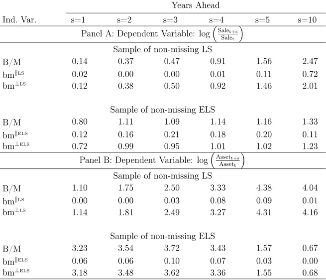
Table VI reports the coefficients of determination (i.e., 𝑅−𝑠𝑞.) attributed to bm‖S and
bm⊥S
in the regressions:
saleg
𝑖,𝑡,𝑡+𝑠 =𝛽0,t+𝛽‖𝑏𝑚𝑖,𝑡+𝜖𝑖,𝑡, (7a) saleg
𝑖,𝑡,𝑡+𝑠 =𝛽0,t+𝛽‖𝑏𝑚
‖𝑆
𝑖,𝑡 +𝛽⊥𝑏𝑚
⊥𝑆
𝑖,𝑡 +𝜖𝑖,𝑡, (7b)
assetg
𝑖,𝑡,𝑡+𝑠 =𝛽0,t+𝛽‖𝑏𝑚𝑖,𝑡 +𝜖𝑖,𝑡, and (8a) assetg
𝑖,𝑡,𝑡+𝑠 =𝛽0,t+𝛽‖𝑏𝑚 ‖𝑆
𝑖,𝑡 +𝛽⊥𝑏𝑚
⊥𝑆
𝑖,𝑡 +𝜖𝑖,𝑡, (8b)
wheresaleg
𝑖,𝑡,𝑡+𝑠 andasset
g
𝑖,𝑡,𝑡+𝑠 are the log sale and asset growth from year𝑡 to year𝑡+𝑠 and
S represents either LS or ELS. The table shows that bm⊥S has significantly more predictive
power over cross-sectional differences in future asset and sales growth than bm‖S, which is
evident from its larger fraction of explained variance. In fact, most of the predictive power
of book-to-market ratios is subsumed by bm⊥S.
II. A Production-Based Model with Labor Leverage and Stochastic
Growth Shocks
We consider an extension of the model in Donangelo et al. (2015) to interpret the
em-pirical findings presented in the previous section. The model incorporates stochastic shocks
to productivity growth that are orthogonal to labor share. Our model highlights the
com-plementary roles of short-term cash-flow volatility and earnings growth in explaining the
cross-section of the book-to-market ratio and expected asset returns. In the model, labor
share affects cash-flow volatility but does not affect earnings growth. Earnings growth, in
turn, is driven by a regime switching process for productivity growth.
A. Setup
We follow Berk et al. (1999) by considering the pricing kernel as exogenous in order to
maintain the tractability of the model and maintain our focus on the effect of micro-level
decisions on firm risk. The dynamics of the pricing kernel Λ are given by
𝑑Λ𝑡 Λ𝑡
=−𝑟𝑑𝑡−𝜂𝑑𝑍𝑡, (9)
where 𝑟 > 0 is the instantaneous risk-free rate and 𝜂 represents the market price of risk in
the economy.
Our setting is neoclassical and represents a firm that employs labor and capital to
pro-duce. A small wage- and price- taking firm has access to a perfectly competitive labor market
composed of a continuum of workers. The dynamics of wages 𝑊 are given by
𝑑𝑊𝑡 𝑊𝑡
=𝜇W𝑑𝑡+𝜎W
√︀ 1−𝜌2
W𝑑𝑍 W
𝑡 +𝜎W𝜌W𝑑𝑍𝑡, (10)
where 𝜇W and 𝜎W are the drift and volatility of wage growth, 𝜌W is its correlation with the
are not priced, (i.e., E[𝑑𝑍W𝑑𝑍]= 0).
Value added by the firm is given by a general constant elasticity of substitution (CES)
production function:
𝑌𝑡=𝐴𝑡𝑋𝑡 (︁
𝛼𝐿 𝜃−1
𝜃
𝑡 + (1−𝛼)𝐾 𝜃−1
𝜃 )︁𝜃−𝜃1
, (11)
where 𝐿 and 𝐾 denote labor and capital employed in production, 𝐴 and 𝑋 denote the
systematic and idiosyncratic components of total factor productivity (TFP), 𝛼 ∈ (0,1)
captures the importance of labor in total production, and𝜃 ∈(0,∞)denotes the elasticity of
substitution between capital and labor.20 The case in which the elasticity𝜃 →0implies that capital and labor are perfect complements. The case in which the elasticity 𝜃 → ∞ implies
that capital and labor are perfect substitutes. The widely used Cobb-Douglas production
function is represented by the special case in which the elasticity 𝜃 → 1. As discussed by
León-Ledesma, McAdam, and Willman (2010); and Klump, McAdam, and Willman (2012);
there is strong empirical evidence in the literature for the case in which the elasticity 𝜃 <1.
Therefore, in this paper, we focus on the case in which𝜃 ∈(0,1).
The systematic and idiosyncratic components of TFP, 𝐴, and𝑋, respectively, follow the
diffusion processes:
𝑑𝐴𝑡 𝐴𝑡
=𝜇A𝑑𝑡+𝜎A𝑑𝑍𝑡, and (12)
𝑑𝑋𝑡 𝑋𝑡
=𝜇X,𝑡𝑑𝑡+𝜎X𝑑𝑍 X
𝑡, (13)
where 𝑑𝑍X
𝑡 is a Wiener process orthogonal to 𝑑𝑍 and 𝑑𝑍
W
(i.e., E[𝑑𝑍X
𝑑𝑍]= 0 and
E[𝑑𝑍X𝑑𝑍W]= 0), and{𝜇
X}t≥0 is a firm-specific two-state Markov process which captures
dif-ferences in the instantaneous growth rates across firms. The state space for𝜇X,𝑡 is {𝜇HX, 𝜇 L X}, 20To isolate the implications of labor share on firm risk, we abstract away from investment and depreciation
where 𝜇H X > 𝜇
L
X. The transition probability of 𝜇X,𝑡 over an infinitesimal time interval 𝑑𝑡 is
given by
⎡
⎣
1−𝜆𝐻𝑑𝑡 𝜆𝐻𝑑𝑡 𝜆𝐿𝑑𝑡 1−𝜆𝐿𝑑𝑡
⎤
⎦, (14)
where 𝜆𝐿 ≥ 0 and 𝜆𝐻 ≥ 0 are the transition intensities from states 𝜇LX to 𝜇 H
X and from 𝜇 H X
to 𝜇L
X, respectively. This transition is assumed to be independent of all other stochastic
processes.
We make several assumptions in our economic setup to ensure the existence of a suitable
solution to our model. These assumptions assure that the value of the firm is bounded, and
they restrict our attention to empirically relevant cases for 𝜃.
Assumption 1
The parameter set {𝑟, 𝜂, 𝜃, 𝜇W, 𝜎W, 𝜌W, 𝜇A, 𝜎A, 𝜇 H X, 𝜇
L
X, 𝜎X, 𝜆H, 𝜆L} is such that Γ1 <0, Γ2 <0,
and 𝜃 < 1. Γ1 and Γ2, which are defined in Appendix A, are constants determined by the
parameter set.
B. Labor Share
The firm determines the optimal level of employment by equating the marginal product
of labor (i.e., 𝑑𝑌𝑡
𝑑𝐿𝑡) to wages 𝑊.
21 The level of labor demanded by the firm, which follows from this optimization, is given by
𝐿*
𝑡 = (︂
1 1−𝛼
)︂1−𝜃𝜃 𝐾
(︃ (︂
𝑊𝑡 𝛼𝐴𝑡𝑋𝑡
)︂1−𝜃 −𝛼
)︃1−𝜃𝜃
. (15)
Note that the optimal labor, 𝐿*
𝑡, equals 0 when the quantity defined above is negative.
This means the firm (temporarily) shuts down because the cost of production exceeds
po-21Perfect labor markets imply that the firm problem of value maximization in this case is analogous to
tential revenue. Next, we define the log labor share as the log of the ratio of labor expenses
to value added, which is given by
𝜓𝑡≡log (︂
𝐿*
𝑡𝑊𝑡 𝑌𝑡
)︂
=𝜃log𝛼+ (1−𝜃) log (︂
𝑊𝑡 𝐴𝑡𝑋𝑡
)︂
, (16)
where the second equality follows from the definition of𝑌 from Equations (11) and (15). A
straightforward application of Ito’s Lemma delivers the dynamics of 𝜓, which are given by
𝑑𝜓𝑡 =𝜇𝜓,𝑡𝑑𝑡+𝜎𝜓W𝑑𝑍 W
𝑡 +𝜎𝜓X𝑑𝑍 X
𝑡 +𝜎𝜓A𝑑𝑍𝑡, (17)
where 𝜇𝜓,𝑡, 𝜎𝜓W, and 𝜎𝜓X, and 𝜎𝜓A are constants defined in Appendix A.
Equations (16) and (17) show that the effect of the two components of productivity, 𝐴
and 𝑋, as well as wages, 𝑊, on labor share is determined by the degree of complementary
between labor and capital (i.e.,𝜃). Given that aggregate wages are smoother than firm-level
productivity (i.e.,𝜎W < 𝜎X, 𝜎A), Equation (16) also highlights that productivity is the main
driver of labor share variation. Moreover, the equation also shows that when labor and
capital are strictly complements (i.e., when the empirically relevant case in which 𝜃 < 1),
labor share is decreasing in the firm’s productivity. The opposite is true when labor and
capital are strictly substitutes (i.e.,𝜃 >1). In the Cobb-Douglas case (i.e.,𝜃 = 1), labor and
capital are neither complements nor substitutes, while labor share is constant and equals 𝛼.
Total operating profits are defined as the residual cash flows of the firm after labor
ex-penses are paid. Using the optimal labor demand (𝐿*𝑡) and the specification of the production
function, we find that operating profits can be expressed as a function of systematic TFP
(𝐴), idiosyncratic TFP (𝑋), and labor share 𝜓, as given by
Π𝑡 = ⎧ ⎨
⎩
(1−𝛼)𝜃−𝜃1𝐴𝑡𝑋𝑡𝐾(︀1−𝑒𝜓𝑡)︀
1 1−𝜃 𝜓
𝑡≤0,
0 otherwise.
The dynamics of profit growth are given by
𝑑Π𝑡 Π𝑡 =
(︂ 1 1−𝑒𝜓𝑡
)︂ (︂
𝑒𝜓𝑡𝜃(𝜎2
A+𝜎
2
W+𝜎
2
X−2𝜌W𝜎A𝜎W)
2(1−𝑒𝜓𝑡) +𝜇A+𝜇X,t−𝑒 𝜓𝑡𝜇
W
)︂
dt (19)
− √︀
1−𝜌2
W𝜎W𝑒
𝜓𝑡 1−𝑒𝜓𝑡 𝑑𝑍
W
𝑡 + 𝜎X
1−𝑒𝜓𝑡𝑑𝑍
X
𝑡 +
(𝜎A−𝜌W𝜎W𝑒𝜓𝑡)
1−𝑒𝜓𝑡 𝑑𝑍𝑡.
Equation (19) shows that the exposure of profit growth to shocks is driven solely by the
level of labor share 𝑒𝜓 and not by the growth regime𝜇
X.22
C. Labor Leverage
Having derived the dynamics of cash flows, we present the mechanism by which labor
share translates into a labor-induced form of operating leverage for the firm. In aggregate
data, corporate profits (or earnings) are highly procyclical and more volatile than TFP or
GDP growth. It is well understood that an important reason for this fact is that labor
compensation is relatively smooth and weakly correlated with TFP or GDP growth.23 To quantify the effect of labor share on firm risk amplification, we define two measures
of the sensitivity of operating profits to each of its two sources of shocks: productivity and
wages. The first is a measure of the sensitivity of cash flow growth to TFP shocks, Θ,
which we denote simply as “operating leverage.” Operating leverage, Θ, is defined, as in
Donangelo (2014), as the scaled covariance of operating profit growth and TFP growth:
Θ ≡ Cov[︀𝑑ΠΠ,𝑑𝑃𝑃 ]︀ ⧸︀Var[︀𝑑𝑃𝑃 ]︀−1, where productivity 𝑃 ∈ {𝐴, 𝑋}.24 Operating leverage is
22The key assumption that makes short-term cash flow risk orthogonal to the growth regime is the absence
of labor adjustment costs. If labor markets are not frictionless, then firms will take into account their growth prospects when deciding how much hiring they will conduct. Our model can be considered the extreme case of what is likely to be a dampened process when frictions are taken into account.
23For instance, Longstaff and Piazzesi (2004) note that “... the reason for the extreme volatility and
procyclicality of corporate earnings is that stockholders are residual claimants to corporate cash flows. Thus, the compensation of workers is a senior claim to cash flows.” See also Gomme and Greenwood (1995).
24Equivalently,Θis defined as the slope of a regression of operating profit growth on TFP growth minus
given by
ΘP
(𝜓𝑡) = 𝑒𝜓𝑡
1−𝑒𝜓𝑡. (20)
Equation (20) shows that the sensitivity of operating profits to TFP growth is positive and
monotonically increasing in labor share 𝑒𝜓𝑡. On the other hand, the sensitivity of operating
profits to wage shocks is given by
ΘW
(𝜓𝑡) =− 1
1−𝑒𝜓𝑡. (21)
Equation (21) shows that the sensitivity of operating profits to wage shocks is negative, and
its magnitude is monotonically increasing in labor share 𝑒𝜓𝑡. These results are summarized
in the proposition below.
Proposition 1
Given Assumption 1, the sensitivity of operating profits to productivity shocks is increasing in the labor share; the sensitivity of operating profits to wage shocks is decreasing in the labor share. Formally,
1. For 𝑃 ∈ {𝐴, 𝑋}, ΘP
(𝜓)>0 and 𝑑Θ𝑑𝜓P(𝜓) >0.
2. ΘW(𝜓)<0 and 𝑑ΘW(𝜓)
𝑑𝜓 <0.
Proof: The Proposition follows directly from Equations (20) and (21).
The previous result characterizes the impact of labor share on operating leverage. The
determinants of labor share, in turn, are determinants of labor-induced operating leverage.
These determinants are the weight of labor in the productive technology production (i.e.,
𝛼) and the level of productivity relative to wages. As labor becomes more important in
production, labor share increases, and operating leverage also increases as a result. In
decrease in operating leverage. These two results, which follow directly from Proposition 1,
are formalized in the following corollary.
Corollary 1
Given Assumption 1, operating leverage is increasing in the importance of labor in production, and decreasing in the level of productivity. Formally,
1. 𝜕Θ𝜕𝛼P(𝜓) >0.
2. For 𝑃 ∈ {𝐴, 𝑋}, 𝜕Θ𝜕𝑃P(𝜓) <0.
Proof: See Appendix C.
Having established the relation between operating leverage and labor share, we now move
on to determining the relation between labor share, firm value, and expected returns. This
is the goal of the following section.
D. Firm Value and Expected Returns
In equilibrium, the value of the firm’s assets (hereafter simply denoted by “firm value”)
equals the value of the discounted stream of optimized operating profits. Firm value (𝑉) is
given by
𝑉[𝐴𝑡, 𝑋𝑡, 𝜓𝑡, 𝜇X,𝑡]≡E𝑡 [︂∫︁ ∞
𝑡 Λ𝑠 Λ𝑡
Π𝑠𝑑𝑠 ]︂
=𝐴𝑡𝑋𝑡𝐾𝑣[𝜓𝑡, 𝜇X,𝑡], (22)
where 𝑣(𝜓𝑡, 𝜇X,𝑡)is given in Appendix B.
The solution for firm value is algebraically intuitive. First, when labor costs become
negligible relative to the value added generated by the firm’s assets (𝜓𝑡 → −∞), firm value
converges to that of the assets of a firm with a dividend equal to 𝐴𝑋𝐾(1−𝛼)𝜃/(𝜃−1). As the cost of labor increases relative to the value added generated by the firm, the dividend falls.
profits are zero, so the firm shuts down production and all firm value arises from the option
to resume production when operating profits become positive again.
The solution has implications for the behavior of the book-to-market ratio as a function
of labor share.25 We show in Appendix D that Assumption 1 implies that 𝑣𝜓(𝜓𝑡, 𝜇X,𝑡) <0.
This result leads to the following proposition.
Proposition 2
Given Assumption 1, a firm’s book-to-market ratio is increasing in labor share. Formally, 𝐵𝑀𝜓[𝐴𝑡, 𝑋𝑡, 𝜓𝑡, 𝜇X,𝑡]>0.
Proof: The Proposition follows directly from 𝑣𝜓[𝜓𝑡, 𝜇X,𝑡]<0.
The result in Proposition 2 implies the existence of a one-to-one correspondence between
the book-to-market ratio (BM) and log labor share 𝜓, given 𝐴, 𝑋, and 𝜇X. Conditional on
the values of𝐴,𝑋, and𝜇X, the problem is invertible so that we can express𝜓, and, therefore,
any weakly monotonic function of𝜓, as a function of BM. One particularly relevant function
for our calculations is the “elasticity of book-to-market with respect to the logarithm of labor
share” (𝜒), which is defined as
𝜒[𝐴𝑡, 𝑋𝑡, 𝐵𝑀𝑡, 𝜇X,𝑡] =
𝐵𝑀𝜓[𝐴𝑡, 𝑋𝑡, 𝜓𝑡, 𝜇X,𝑡] 𝐵𝑀[𝐴𝑡, 𝑋𝑡, 𝜓𝑡, 𝜇X,𝑡]
. (23)
The elasticity𝜒determines whether instantaneous expected asset returns increase or decrease
as labor share increases. Formally, expected returns are defined as the instantaneous drift
of the gains process that reinvests dividends, Et[𝑅𝑡]≡Et [︁
𝑑𝑉𝑡+Π𝑡𝑑𝑡 𝑉𝑡
]︁
, and are given by
E[𝑅𝑡|𝜓𝑡, 𝜇X,𝑡] =𝑟+𝜂𝜎A+𝜂(𝜎A−𝜌W𝜎W) (1−𝜃)𝜒[𝐴𝑡, 𝑋𝑡, 𝐵𝑀𝑡, 𝜇X,𝑡]. (24)
Equation (24) links the expected returns of the firm directly to the elasticity 𝜒. From
Proposition 2, it follows that 𝜒 is positive and, therefore, induces a risk premium. The risk
25The book-to-market ratio is defined as book value over market value (or simply “value”) of assets.
premium induced will be a function of the expected growth rate of the firm 𝜇X, the firm’s
labor share and its book-to-market ratio.26
A more relevant question for our study is the change in expected returns as a function of
book-to-market. If the elasticity 𝜒 increases with book-to-market, then the model predicts
the existence of a value premium. We show that this is true in at least part of the range for
labor share. The result is characterized below.
Proposition 3
Given Assumption 1 and 𝜎A > 𝜌W𝜎W, a firm’s systematic risk loading is increasing in the
logarithm of labor share in some interval (−∞, 𝜅). More precisely, 𝜕E[𝑅𝑡|𝜓,𝜇X,𝑡]
𝜕𝜓 > 0 in the interval 𝜓 ∈(−∞, 𝜅), where 𝜅 is a real valued function defined in Appendix E.
Proof: See Appendix E.
Proposition 3 implies that the relation between risk and labor share depends on the sign
of 𝜎A−𝜌W𝜎W (i.e., it depends on the procyclicality of productivity with respect to wages).
To better understand this result, we analyze the implications derived from Equation (24)
in more detail. Equation (24) shows that the firm’s excess returns over the risk-free rate
depend on two drivers of systematic risk loadings. The first driver is the covariance between
the firm’s productivity and the stochastic discount factor (𝜂𝜎A). We call this theproductivity
lever of systematic risk loadings. The productivity lever affects expected returns directly through its impact on overall productivity, and indirectly through its impact on the relative
productivity of capital and labor. It is this second, and indirect, component that depends on
the firm’s labor share. The direct impact of the productivity lever for an average firm will
be positive, as it produces more, or as the prices of its products increase in good times. The
indirect impact is also positive, since our assumption of the complementarity between labor
and capital implies that a positive shock to the firm’s productivity will amplify the impact
on profits.
26To illustrate this, note that logarithm of labor share𝜓 is not instantaneously affected by a change in
productivity growth𝜇X from𝜇HXto 𝜇 L
The second driver of systematic risk loading captures the firm’s exposure to aggregate
wages (𝜌W𝜎W). We call this component the wage hedge, as it depends only on the firm’s
exposure to wages and will likely reduce the risk for the average firm. The wage hedge is related to a firm’s labor share because variations in wages will have a larger effect on firms
for which most of their value added is used to pay for labor. This component is a hedge
because, on average, wages fall in bad times, which is precisely when firm’s profits are falling
due to systematic falls in their own productivity.
Combining the two drivers of systematic risk loadings–one positive (the productivity
lever), the other negative (the wage hedge)–delivers the relation between the firm’s labor
share and expected returns. The relation will be positive if the firm’s systematic component
of productivity is procyclical enough with respect to wages. For instance, a firm with
pro-ductivity that is uncorrelated with the stochastic discount factor (𝜎A = 0) has a systematic
risk loading that is decreasing in its labor share. In this case, the hedge effect of wages
is uncontested: In good times, wages go up, so profits fall. In bad times, wages go down,
and the firm’s profits increase. The hedging impact of wages, though, is muted when the
firmâĂŹs productivity is sufficiently procyclical (𝜎A > 𝜌W𝜎W). In this case, even though
wages are a hedge, the procyclical variation in the firm’s sales price dominates, making the
firm riskier as its labor share increases.
E. A Numerical Example
The previous section derived the general solution for the value of the firm as a function
of its labor share Ψ ≡ 𝑒𝜓. In this section, we use a numerical example to illustrate the
relationship between labor share, productivity, wages, firm value, labor leverage, and betas.
We study the case in which the elasticities of substitution 𝜃 = 0.5, which is in the range of
what many empirical studies find for the elasticity of substitution between capital and labor.
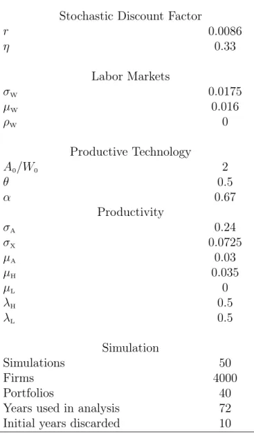
The parameter values used in this example are presented in Table VII.
id-iosyncratic productivity and wages. The top panel shows that labor shares are decreasing
in productivity. The bottom panel of Figure (1) shows that labor share is increasing in
economy-wide wages. The flat portion of the plots represents states in which the firm shuts
down to prevent paying over 100% of value added to labor. The negative relationship between
labor shares and productivity and the negative relationship between labor shares and wages
are driven by two key assumptions in our model. The first is that there are no frictions in
labor markets, so labor earns economy-wide wages. The second assumption is that the
elas-ticity of substitution between labor and capital is strictly less than unit so that the marginal
product of capital (MPK) is decreasing in wages. Taken together, these assumptions imply
that there will be imperfect sharing of productivity shocks between workers and the owners
of capital. When productivity is low relative to wages, some workers leave, which decreases
MPK so that labor shares increase. Similarly, the firm can easily hire more workers when
productivity is high, which increases MPK so that labor shares fall. If labor were completely
immobile, labor supply would not be affected by economy-wide wages, so labor shares would
not be affected by productivity. Similarly, when the elasticity of substitution between labor
and capital is equal to 1, then MPK and labor share are unaffected by wages and
productiv-ity. In the case in which the elasticity of substitution between labor and capital is greater
than 1, the mechanism described above is reversed.
<<
Figure 1 here
>>
Figure (2) shows the negative relation between labor shares, profits, and firm value. As
the firm becomes less productive or as wages increase (i.e., as labor share increases), a larger
share of output is used to compensate labor so that operating profits decline. The negative
relation between labor shares and firm value is due to two channels: a cash flow channel and
a discount rate channel. The cash flow channel is related to lower operating profits of
discount rate channel is related to the higher loading on systematic risk of a high-labor-share
firm relative to a low-labor-share firm. The bottom panel of Figure (2) shows the value of
the firm under the two growth regimes. This panel illustrates that the drop in firm value
due to a change from the high to the low growth states is relatively unaffected by the level
of labor share of the firm.
<<
Figure 2 here
>>
Figure (3) sheds some light on the relation between labor share and the exposure of
operating profits to the two sources of uncertainty in the model: productivity and wages.
This figure shows that the sensitivity of operating profits to both productivity and wage
shocks is increasing in labor share. This effect, which corresponds to what we have denoted
as labor leverage, is an intuitive result: Higher labor shares are related to lower profit
margins, which buffer the firm against either type of shock. Productivity is positively related
to operating profits, so that the exposure to productivity shocks is always positive and
increasing in labor share. Labor expenses are negatively related to operating profits, so that
the exposure to wage shocks is always negative and its magnitude is increasing in labor share.
<<
Figure 3 here
>>
Figure (4) shows the relation between book-to-market ratio, productivity, and labor
share. The plot shows that the book-to-market ratio is negatively related to productivity
and, therefore, positively related to labor share. Moreover, the plots show how the
book-to-market ratio is negatively affected by a low growth regime. The effect of labor share on
the book-to-market ratio is more pronounced under the low-growth regime than under the
<<
Figure 4 here
>>
Figure (5) illustrates the discount rate channel. The figure shows that the beta is
de-creasing in productivity and therefore inde-creasing in labor share. The figure also shows how
the beta is affected by the different growth regimes. In particular, the figure shows that
betas are higher under the low growth regime and shows that this effect is increasing in
labor share and decreasing in productivity.
The figure highlights that the labor leverage mechanism is conceptually similar to
op-erating leverage due to fixed opop-erating expenses, even though all costs are variable in our
model. Also, note that the labor leverage mechanism does not require any assumptions
about the relative riskiness of wages and productivity, although the assumption about the
relative procyclicality of wages and productivity is necessary to obtain a positive relation
between labor leverage and systematic risk loadings. When productivity is less procyclical
than wages, then high-labor-share firms have lower exposure to systematic risk, although
they also have narrower profit margins. The overall effect on firm value when productivity
is less procyclical than wages depends on the relative magnitude of the lower profit margins
(i.e., the cash flow effect) and the lower loadings on systematic risk (i.e., the discount rate
channel) of high-labor-share firms.
<<
Figure 5 here
>>
F. Labor Share and the Value Spread
F.1. Simulation Exercise
The analysis of our model so far implicitly treats labor share as exogenously given. To
endogenous relationship between labor share, book-to-market ratios, earnings, and expected
asset returns. To do so, we conduct a simulation exercise with a large cross-section of firms
in which the labor share and our variables of interest are jointly determined. Moreover,
the use of the model to generate artificial data allows us to extend the methodology in
CPV to decompose the cross-sectional variance of book-to-market ratios into components
that are explained by differences in expected returns and by differences in earnings growth.
The component of book-to-market ratio variance related to expected future returns is, in a
sense, the definition of the value premium. Therefore, we quantify the extent to which labor
share explains the value premium by measuring the relation between labor share and the
component of book-to-market ratio variance related to expected future returns.
We investigate the endogenous relation between labor share and our variables of interest
in a numerical simulation of the model. We conduct 50 runs of a cross-section of 4,000
firms over 72 years. Firms are identical at the beginning of our simulation, so we discard
the first 10 years of simulated data to ensure cross-sectional heterogeneity that arises from
differences in the idiosyncratic shock paths. The number of firms is representative of the
number of publicly traded firms in the United States at any point. The chosen net time span
corresponds to the time frame of the empirical sample for which we can compare the results
later (i.e., 1950–2012).
We chose the parameters in the simulation as follows. Based on historical data, we fix the
risk-free rate at 0.86%, wage growth at 1.6%, and wage volatility at 1.75%. We set𝜂to match
empirically observed values of the Sharpe ratio (.33). And, lacking appropriate empirical
counterparts, we set the correlation between wage growth and the stochastic discount factor
at 0. Without loss of generality, we set the initial value of idiosyncratic productivity 𝑋0
and the capital stock 𝐾 to 1, and we set the growth rate of firms in the low-growth regime
to 0. We then search parameters for systematic volatility 𝜎A, idiosyncratic volatility 𝜎X,
economy-wide growth rate 𝜇A, and earnings growth in the high-growth regime 𝜇h, that can
along with other empirical results. However, note that we calibrate our simulation to best
match those results. Finally, we set the initial values of aggregate productivity𝐴0 and wage
rate 𝑊0 so that the average firm’s labor share and book-to-market ratio over the simulated
period match the empirical sample’s data.
In addition to the previous parameters, which are all found in the model, we include
an idiosyncratic shock since we recognize that the econometrician encounters measurement
error when measuring the variables of interest in the model. We focus the shock on the
measurement of labor share while assuming that everything else is measured perfectly. The
inclusion of measurement error is crucial for some of the results we describe below. Without
measurement error, the relation between labor share and the book-to-market ratio becomes
very close. In this case, the labor share almost completely explains the book-to-market ratio,
which is counterfactual. We use a unit-root process for the error with a volatility parameter
of 1.1.
Table VII reports the resulting parameters. In order to match the empirical results more
closely, we find relatively high systematic volatility𝜎A(24%) and relatively low idiosyncratic
volatility 𝜎X (7.25%). Low values for𝜎A, which are implied by low productivity volatility at
the aggregate level, lower the fraction of the book-to-market variance explained by future
returns in the model. This is contrary to what we find empirically. Low values of𝜎X, on the
other hand, increase the fraction of the book-to-market variance explained by future returns
in the model, so increasing 𝜎X lowers the fraction of book-to-market variance explained by
future returns, which also contradicts what we find empirically.
<<
Table VII here
>>
Why does systematic volatility𝜎A and idiosyncratic volatility𝜎X have a different impact
on the capacity of future returns to explain variance in the cross-section of book-to-market
returns to explain the book-to-market variance. In the limit, when 𝜎X = 0, all firms in the
same growth regime move in lockstep, and the only difference in returns in the cross-section
of returns will be due to differences in initial labor shares and growth rate regimes. The
to-market ratios will also move in lockstep, implying a tight relation between
book-to-market ratio and future returns. This relation weakens once 𝜎X > 0, as now firms do
not move in lockstep. A high-labor-share firm may find itself with lower labor share a few
years later, even though most other firms have increased their labor shares. Thus, the link
between future returns and book-to-market ratios will weaken.
The values for productivity growth in the high- and low-growth regimes, as well as the
associated transition probabilities, determine how much future earnings growth explains the
components bm‖LS
and bm⊥LS
. In general, higher spreads between expected growth rates, or
lower probabilities of switching states, lead to an increase in the variance of book-to-market
ratios explained by future earnings. The effect is strongest when explaining bm⊥LS, since the
growth differences between the regimes do not cause a change in labor share. The resulting
values in the calibration are a growth spread of 3.5%, and jump intensities of 0.5 for both𝜆H
and𝜆L. These jump intensities imply that a regime shift from high to low growth is expected
to occur once every two years.
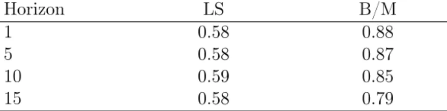
Table VIII reports the summary statistics of our simulation. The average labor share
during these 62 years is .59 and is relatively constant over the sample period considered.
The average book-to-market ratio varies according to the horizon: It is .88 for the entire
sample period at the 1-year horizon and falls to .79 at the 3- and 15-year horizon. The
empirical counterparts for the sample reporting wages is .60 for the labor share and .82 for
the book- to-market ratio. In this table, we do not report the volatilities of labor share and
the labor market. We find that the volatilities in our simulation are roughly half as high as
the volatilities we find in the data.
After generating simulated values and dividends in our simulation, we now study the
explanatory power of the simulated data in understanding the relation between labor share,
book-to-market, future returns, and earnings growth. The analysis follows the procedure
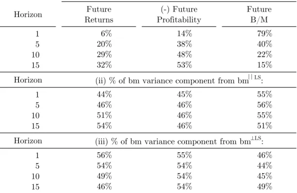
described in Equations (3), (4), and (5). The fraction of the book-to-market volatility
ex-plained by future earnings and future returns grows with the time horizon and is significantly
higher for future earnings than future returns. At a 15-year horizon, future returns explain
32% of the book-to-market variance, whereas future earnings explain 53%. The remaining
15% is residual captured by future book-to-market. Thus, the model succeeds in
qualita-tively replicating the results found in CPV. In particular, future returns and future earnings
growth explain a significant fraction of book-to-market variance over long horizons.
More-over, future earnings growth explains roughly twice as much of the book-to-market ratio
variance as future returns.
The middle and lower panels of Table IX show the results of the same analysis, except that
the variance being explained is that of bm‖LS
(the component of book-to-market explained
by labor share) and of bm⊥LS(the component of book-to-market orthogonal to labor share).
Both of these are normalized by the values presented in the top panel. At the 15-year horizon,
future returns explain 23% of the variance in book-to-market ratio (as seen in the top panel,
second column). The middle panel shows that, at the same 15-year horizon, 41.11% of the
23% (i.e., about 10%) is the amount future returns explained by variance in bm‖LS
. The lower
panel shows that 58.89% of the 23% (i.e., about 13%), is the variance of bm⊥LSexplained by
future returns. The corresponding empirical values for our LS measure (Table II, Panel A),
are 54% and 46%, respectively. Thus, our simulated results, though not quite identical to
the data, deliver similar qualitative results: The variance of bm‖LSand bm⊥LSexplained by
future returns is roughly the same.
Shifting our attention to the next panel, we observe that at the 15-year horizon, future
earnings growth explain 48% of the variance in book-to-market ratios. The middle panel
that future earnings explain the variance of bm‖LS. The lower panel shows that 75.5%
of the 48% (i.e., about 36%), is the variance of bm⊥LS
explained by future earnings. The
corresponding empirical values, for our LS measure (Table II, Panel A) are 15% and 84%,
respectively. Our simulated results imply that bm⊥LS
explains around three-quarters of the
relation between variance in book-to-market ratio and variance in future earnings.
Conclusion
We provide evidence that the value premium is driven by both differences in cash flow
risk and differences in future growth opportunities. Our method relies on the observation
that a firm’s labor share induces operating leverage, and thus is related to cash flow risk. A
direct implication of this observation is that labor share is a firm characteristic that should
explain the cross-section of returns and help us understand the drivers of the value premium.
Our empirical findings add to our understanding of the predictive power of
book-to-market ratios on future returns and cash flows. In particular, the use of labor share allowed
us to explore the different implications that book-to-market ratios have on a firm’s riskiness
and growth prospects. We find that the component of valuations explained by the labor
share is significantly related to expected returns, linking labor share to risk but not to future
earnings growth. In contrast, the component of valuations not explained by the labor share
is significantly related to future earnings. Thus, labor share allows us to disentangle sources
of variation in book-to-market ratios between risk-based and growth-basted explanations.
Overall, we find that labor share explains approximately 50% of the variation in
book-to-market ratios that are attributable to future returns (i.e., the value premium).
We develop a simple stylized production-based model of a firm to study the labor leverage
mechanism. The model allows us to explore the risk, return, and growth dynamics as a
function of labor share. Crucially, the model makes explicit two distinct drivers of
book-to-market values: one related to labor share (through labor leverage), and the other unrelated to
labor share (through growth expectations). It is worth mentioning again that our theoretical
setup is frictionless, and we abstract away from any variations that derive from capital (e.g.,
investments). Nevertheless, the simulation results suggest that our parsimonious model is
able to explain the book-to-market variance decomposition from CPV. Moreover, this simple
setting can replicate the main features in the data that correspond to the relation between