PubMedCentral-PMC5658064.pdf

(1)

CGC: A Flexible and Robust Approach to Integrating

Co-Regularized Multi-Domain Graph for Clustering

Wei Cheng, UNC at Chapel Hill

Zhishan Guo, UNC at Chapel Hill

Xiang Zhang, and

Case Western Reserve University

Wei Wang

University of California, Los Angeles

Abstract

Multi-view graph clustering aims to enhance clustering performance by integrating heterogeneous information collected in different domains. Each domain provides a different view of the data instances. Leveraging cross-domain information has been demonstrated an effective way to achieve better clustering results. Despite the previous success, existing multi-view graph clustering methods usually assume that different views are available for the same set of instances. Thus instances in different domains can be treated as having strict one-to-one relationship. In many real-life applications, however, data instances in one domain may correspond to multiple instances in another domain. Moreover, relationships between instances in different domains may be associated with weights based on prior (partial) knowledge. In this paper, we propose a flexible and robust framework, CGC (Co-regularized Graph Clustering), based on non-negative matrix factorization (NMF), to tackle these challenges. CGC has several advantages over the existing methods. First, it supports many-to-many cross-domain instance relationship. Second, it incorporates weight on cross-domain relationship. Third, it allows partial cross-domain mapping so that graphs in different domains may have different sizes. Finally, it provides users with the extent to which the cross-domain instance relationship violates the in-domain clustering structure, and thus enables users to re-evaluate the consistency of the relationship. We develop an efficient optimization method that guarantees to find the global optimal solution with a given confidence requirement. The proposed method can automatically identify noisy domains and assign smaller weights to them. This helps to obtain optimal graph partition for the focused domain. Extensive experimental results on UCI benchmark data sets, newsgroup data sets and biological interaction networks demonstrate the effectiveness of our approach.

Author’s addresses: W. Cheng and Z. Guo, Department of Computer Science, University of North Carolina at Chapel Hill; X. Zhang,

HHS Public Access

Author manuscript

ACM Trans Knowl Discov Data

. Author manuscript; available in PMC 2017 October 26.

Published in final edited form as:

ACM Trans Knowl Discov Data. 2016 July ; 10(4): . doi:10.1145/2903147.

(2)

Additional Key Words and Phrases

graph clustering; nonnegative matrix factorization; co-regularization

General Terms

Design; Algorithms; Performance

1. INTRODUCTION

Graphs are ubiquitous in real-life applications. A large volume of graph data have been generated, such as social networks [Leskovec et al. 2007], biology interaction networks [Fenyo 2010], and literature citation networks [Sun and Han 2012]. Graph clustering has attracted increasing research interest recently. Several effective approaches have been proposed in the literature, such as spectral clustering [Ng et al. 2001], symmetric Non-negative Matrix Factorization (symNMF) [Kuang et al. 2012], Markov clustering (MCL) [van Dongen 2000].

In many applications, graph data may be collected from heterogeneous domains (sources) [Gao et al. 2009]. For example, the gene expression levels may be reported by different techniques or on different sample sets, thus the gene co-expression networks built on them are heterogeneous; the proximity networks between researchers such as co-citation network and co-author network are also heterogeneous. By exploiting multi-domain information to refine clustering and resolve ambiguity, multi-view graph clustering methods have the potential to dramatically increase the accuracy of the final results [Bickel and Scheffer 2004; Kumar et al. 2011; Chaudhuri et al. 2009]. The key assumption of these methods is that the same set of data instances may have multiple representations, and different views are generated from the same underlying distribution [Chaudhuri et al. 2009]. These views should agree on a consensus partition of the instances that reflects the hidden ground truth [Long et al. 2008]. The learning objective is thus to find the most consensus clustering structure across different domains.

Existing multi-view graph clustering methods usually assume that information collected in different domains are for the same set of instances. Thus, the cross-domain instance relationships are strictly one-to-one. This also implies that different views are of the same size. For example, Fig. 1(a) shows a typical scenario of multi-view graph clustering, where the same set of 12 data instances has 3 different views. Each view gives a different graph representation of the instances.

In many real-life applications, it is common to have cross-domain relationship as shown in Fig. 1(b). This example illustrates several key properties that are different from the traditional multi-view graph clustering scenario.

• An instance in one domain may be mapped to multiple instances in another domain. For example, in Fig. 1(b), instance Ⓐ A in domain 1 is mapped to two

A

uthor Man

uscr

ipt

A

uthor Man

uscr

ipt

A

uthor Man

uscr

ipt

A

uthor Man

uscr

(3)

instances ➀ and ➁ in domain 2. The cross-domain relationship is many-to-many rather than one-to-one.

• Mapping between cross-domain instances may be associated with weights, which is a generalization of a binary relationship. As shown in Fig. 1(b), each cross-domain mapping is coupled with a weight. Users may specify these weights based on their prior knowledge.

• The cross-domain instance relationship may be a partial mapping. Graphs in different domains may have different sizes. Some instance in one domain may not have corresponding instance in another. As shown in Fig. 1(b), mapping between instances in different domains is not complete.

One important problem in bioinformatics research is protein functional module detection [Hub and de Groot 2009]. A widely used approach is to cluster protein-protein interaction (PPI) networks [Asur et al. 2007]. In a PPI network, each instance (node) is a protein and an edge represents the strength of the interaction between two connected proteins. To improve the accuracy of the clustering results, we may explore the data collected in multiple domains, such as gene co-expression networks [Horvath and Dong 2008] and genetic interaction networks [Cordell 2009]. The relationship across gene, protein and genetic variant domains can be many-to-many. For example, multiple proteins may be synthesized from one gene and one gene may contain many genetic variants. Consider another

application of text clustering, where we want to cluster journal paper corps (domain 1) and conference paper corps (domain 2). We may construct two affinity (similarity) graphs for domains 1 and 2 respectively, in which each instance (node) is a paper and an edge

represents the similarity between two papers (e.g., cosine similarity between term-frequency vectors of the two papers). Some journal papers may be extended versions of one or multiple conference papers. Thus the mappings between papers in two domains may be many-to-many.

These emerging applications call for novel cross-domain graph clustering methods. In this paper, we propose CGC (Co-regularized Graph Clustering), a flexible and robust approach to integrate heterogenous graph data. Our contributions are summarized as follows.

1. We propose and investigate the problem of clustering multiple heterogenous graph data, where the cross-domain instance relationship is many-to-many. This problem has a wide range of applications and poses new technical challenges that cannot be directly tackled by traditional multi-view graph clustering methods.

2. We develop a method, CGC, based on collective symmetric non-negative matrix factorization with co-regularized penalty to manipulate cross-domain

relationships. CGC allows weighted cross-domain relationships. It also allows partial mapping and can handle graphs with different sizes. Such flexibility is crucial for many real-life applications. We also provide rigid theoretical analysis of the performance of the proposed method.

3. We develop an efficient optimization method for CGC by population-based Tabu Search, and further extended it into a parallel algorithm. It guarantees to find the global optimum with a given confidence requirement.

(4)

4. We develop effective and efficient techniques to handle the situation when the cross-domain relationship contains noise. Our method supports users to evaluate the accuracy of the specified relationships based on single-domain clustering structure. For example, in Fig. 1(b), mapping between (Ⓑ – ➂) in domains 1 and 2, and (➄ – ⓐ) in domains 2 and 3, may not be accurate as they are

inconsistent with in-domain clustering structure. (Note that each domain contains two clusters, one on the top and one at the bottom.)

5. We provide effective techniques to automatically identify noisy domains. By assigning smaller weights to noisy domains, the CGC algorithm can obtain optimal graph partition for the focused domain.

6. We evaluate the proposed method on benchmark UCI data sets, newsgroup data sets and various biological interaction networks. The experimental results demonstrate the effectiveness of our method.

2. PROBLEM FORMULATION

Suppose that we have d graphs, each from a domain in { 1, 2,..., d}. We use nπ to denote

the number of instances (nodes) in the graph from domain _π (1 ≤ π ≤ d). Each graph is represented by an affinity (similarity) matrix. The affinity matrix of the graph in domain _π is denoted as . In this paper, we follow the convention and assume that A(π) is a symmetric and non-negative matrix [Ng et al. 2001; Kuang et al. 2012]. We denote the set of pairwise cross-domain relationships as ℐ = {(i, j)} where i and j are domain indices. For example, ℐ = {(1, 3), (2, 5)} contains two cross-domain relationships (mappings): the relationship between instances in 1 and 3, and the relationship between instances in 2

and 5. Each relationship (i, j) ∈ℐ is coupled with a matrix , indicating the

(weighted) mapping between instances in i and j, where ni and nj represent the number of

instances in i and j respectively. We use to denote the weight between the a-th

instance in j and the b-th instance in i, which can be either binary (0 or 1) or quantitative

(any value between [0,1]). Important notations are listed in Table I.

Our goal is to partition each A(π) into k_π clusters while considering the co-regularizing constraints implicitly represented by the cross-domain relationships in ℐ.

3. CO-REGULARIZED MULTI-DOMAIN GRAPH CLUSTERING

In this section, we present the Co-regularized Graph Clustering (CGC) method. We model cross-domain graph clustering as a joint matrix optimization problem. The proposed CGC method simultaneously optimizes the empirical likelihood in multiple domains and take into account the cross-domain relationships.

3.1. Objective Function

3.1.1. Single-Domain Clustering—Graph clustering in a single domain has been extensively studied. We adopt the widely used non-negative matrix factorization (NMF) approach [Lee and Seung 2000]. In particular, we use the symmetric version of NMF

(5)

[Kuang et al. 2012; Ding et al. 2006] to formulate the objective of clustering on A(π) as minimizing the objective function:

(1)

where || · ||F denotes the Frobenius norm, H(π) is a non-negative matrix of size nπ × kπ, and

k_π is the number of clusters requested. We have , where each represents the cluster assignment (distribution) of the a-th

instance in domain _π. For hard clustering, is often used as the cluster assignment.

3.1.2. Cross-Domain Co-Regularization—To incorporate the cross-domain

relationship, the key idea is to add pairwise co-regularizers to the single-domain clustering objective function. We develop two loss functions to regularize the cross-domain clustering structure. Both loss functions are designed to penalize cluster assignment inconsistency with the given cross-domain relationships. The residual sum of squares (RSS) loss requires that graphs in different domains are partitioned into the same number of clusters. The clustering disagreement loss has no such restriction.

A). Residual sum of squares (RSS) loss function: We first consider the case where the number of clusters is the same in different domains, i.e. k1 = k2 = ... = kd = k. For simplicity,

we denote the instances in domain _π as { }. If an instance in i is

mapped to an instance in j, then the clustering assignments and should be

similar. We now generalize the relationship to many-to-many. We use to denote

the set of indices of instances in i that are mapped to with positive weights, and

represents its cardinality. To penalize the inconsistency of cross-domain cluster partitions, for the l-th cluster in i, the loss function (residual) for the b-th instance is

(2)

where

(3)

is the weighted mean of cluster assignment of instances mapped to , for the l-th cluster.

A

uthor Man

uscr

ipt

A

uthor Man

uscr

ipt

A

uthor Man

uscr

ipt

A

uthor Man

uscr

(6)

We assume every non-zero row of S(i,j) is normalized. By summing up Eq. (2) over all instances in j and k clusters, we have the following residual of sum of squares loss function

(4)

B). Clustering disagreement (CD) loss function: When the number of clusters in different domains varies, we can no longer use the RSS loss to quantify the inconsistency of cross-domain partitions. From the previous discussion, we observe that S(i,j)H(i) in fact serves as a weighted projection of instances in domain i to instances in domain j. For simplicity, we

denote the matrix H̃(i→j) = S(i,j)H(i). Recall that represents a cluster assignment over kj

clusters for the a-th instance in j. Then corresponds to for the a-th instance in

domain j. The previous RSS loss compares them directly to measure the clustering

inconsistency. However, it is inapplicable to the case where different domains have different

numbers of clusters. To tackle this problem, we first measure the similarity between

and , and the similarity between and . Then we measure the difference between these two similarity values. Taking Fig. 1(b) as an example. Note that Ⓐ and Ⓑ; in domain 1 are mapped to ➁ in domain 2, and Ⓒ is mapped to ➃. Intuitively, if the

similarity between clustering assignments for ➁ and ➃ is small, the similarity of clustering assignments between Ⓐ and Ⓒ and the similarity between Ⓑ; and Ⓒ should also be small. Note that symmetric NMF can handle both linearity and nonlinearity [Kuang et al. 2012]. Thus in this paper, we choose a linear kernel to measure the in-domain cluster

assignment similarity, i.e., . The cross-domain clustering disagreement loss function is thus defined as

(5)

3.1.3. Joint Matrix Optimization—We can integrate the domain-specific objective and the loss function quantifying the inconsistency of cross-domain partitions into a unified objective function

(6)

A

uthor Man

uscr

ipt

A

uthor Man

uscr

ipt

A

uthor Man

uscr

ipt

A

uthor Man

uscr

(7)

where (i,j) can be either or . λ(i,j) ≥ 0 is a tuning parameter balancing between in-domain clustering objective and cross-domain regularizer. When all λ(i,j)= 0, Eq. (6) degenerates to d independent graph clusterings. Intuitively, the more reliable the prior cross-domain relationship, the larger the value of λ(i,j).

3.2. Learning Algorithm

In this section, we present an alternating scheme to optimize the objective function in Eq. (6), that is, we optimize the objective with respect to one variable while fixing others. This procedure continues until convergence. The objective function is invariant under these updates if and only if H(π)’s are at a stationary point [Lee and Seung 2000]. Specifically, the solution to the optimization problem in Eq. (6) is based on the following two theorems, which is derived from the Karush-Kuhn-Tucker (KKT) complementarity condition [Boyd and Vandenberghe 2004]. Detailed theoretical analysis of the optimization procedure will be presented in the next section.

Theorem 3.1: For RSS loss, updating H(π) according to Eq. (7) will monotonically decrease the objective function in Eq. (6) until convergence.

(7)

where

(8)

and

(9)

Theorem 3.2: For CD loss, updating H(π)_{according to Eq. (10) will monotonically decrease}

the objective function in Eq. (6) until convergence.

(10)

A

uthor Man

uscr

ipt

A

uthor Man

uscr

ipt

A

uthor Man

uscr

ipt

A

uthor Man

uscr

(8)

where

(11)

and

(12)

where ∘, and are element-wise operators.

Based on Theorem 3.1 and Theorem 3.2, we develop the iterative multiplicative updating algorithm for optimization and summarize it in Algorithm 1.

Algorithm 1

Co-regularized Graph Clustering (CGC)

3.3. Theoretical Analysis

3.3.1. Derivation—We derive the solution to Eq. (6) following the constrained optimization theory [Boyd and Vandenberghe 2004]. Since the objective function is not

A

uthor Man

uscr

ipt

A

uthor Man

uscr

ipt

A

uthor Man

uscr

ipt

A

uthor Man

uscr

(9)

jointly convex, we adopt an effective alternating minimization algorithm to find a locally optimal solution. We prove Theorem 3.2 in the following. The proof of Theorem 3.1 is similar and hence omitted.

We formulate the Lagrange function for optimization

(13)

Without loss of generality, we only show the derivation of the updating rule for one domain

π (π∈ [1, d]). The partial derivative of Lagrange function with respect to H(π)_is:

(14)

Using the Karush-Kuhn-Tucker (KKT) complementarity condition [Boyd and Vandenberghe 2004] for the non-negative constraint on H(π), we have

(15)

The above formula leads to the updating rule for H(π) in Eq. (10).

3.3.2. Convergence—We use the auxiliary function approach [Lee and Seung 2000] to prove the convergence of Eq. (10) in Theorem 3.2. We first introduce the definition of auxiliary function as follows.

Definition 3.1: Z(h, h̃) is an auxiliary function for L(h) if the conditions

(16)

are satisfied for any given h, h̃ [ Lee and Seung 2000].

A

uthor Man

uscr

ipt

A

uthor Man

uscr

ipt

A

uthor Man

uscr

ipt

A

uthor Man

uscr

(10)

Lemma 3.1: If Z is an auxiliary function for L, then L is non-increasing under the update [Lee and Seung 2000].

(17)

Theorem 3.3: Let L(H(π)) denote the sum of all terms in L containing H(π). The following function

(18)

is an auxiliary function for L(H(π)_{), where} _{and Q(j)}

= (H̃(π))T(S(π,j))TS(π,j)H̃(π)(H̃(π))T(S(π,j))TS(π,j). Furthermore, it is a convex function in H(π) and has a global minimum.

Theorem 3.3 can be proved using a similar idea to that in [Ding et al. 2006] by validating Z(H(π)_{, H}̃(π)_{) ≥ L(H}(π)_{), Z(H}(π)_{, H}(π)_{) = L(H}(π)_{), and the Hessian matrix}_∇∇

H(π)Z(H(π),

H̃(π)) ⪰ 0. Due to space limitation, we omit the details.

Based on Theorem 3.3, we can minimize Z(H(π)_{, H}̃(π)_{) with respect to H}(π)_{with H}̃(π)

fixed. We set ∇H(π)Z(H(π), H̃(π)) = 0, and get the following updating formula

which is consistent with the updating formula derived from the KKT condition aforementioned.

From Lemma 3.1 and Theorem 3.3, for each subsequent iteration of updating H(π), we have L((H(π)₎0_{) = Z((H}(π)₎0_{, (H}(π)₎0_{) ≥ Z((H}(π)₎1_{, (H}(π)₎0_{) ≥ Z((H}(π)₎1_{, (H}(π)₎1_{) = L((H}(π)₎1₎

≥ ... ≥ L((H(π)₎Iter_{). Thus L(H}(π)_{) monotonically decreases. This is also true for the other}

A

uthor Man

uscr

ipt

A

uthor Man

uscr

ipt

A

uthor Man

uscr

ipt

A

uthor Man

uscr

(11)

variables. Since the objective function Eq. (6) is lower bounded by 0, the correctness of Theorem 3.2 is proved. Theorem 3.1 can be proven with a similar strategy.

3.3.3. Complexity Analysis—The time complexity of Algorithm 1 (for both loss functions) is (Iter · d|ℐ|(ñ3_{+ ñ}2_k̃_{)), where ñ is the largest n}

π (1 ≤ π ≤ d), k̃ is the largest k_π and Iter is the number of iterations needed before convergence. In practice, |ℐ| and d are usually small constants. Moreover, from Eq. (10) and Eq. (7), we observe that the ñ3_{term is}

from the matrix multiplication (S(π,j))TS(π,j). Since S(π,j) is the input matrix and often very sparse, we can compute (S(π,j))TS(π,j) in advance in sparse form. In this way, the complexity of Algorithm 1 is reduced to (Iter · ñ2k̃).

3.4. Finding Global Optimum

The objective function Eq. (6) is a fourth-order non-convex function with respect to H(π). The achieved stationary points (satisfying KKT condition in Eq. (15)) may not be the global optimum. Many methods have been proposed in the literature to avoid local optima, such as Tabu search [Glover and McMillan 1986], particle swarm optimization (PSO) [Dorigo et al. 2008], and estimation of distribution algorithm (EDA) [Larraanaga and Lozano 2001]. Since our objective function is continuously differentiable over the entire parameter space, we develop a learning algorithm for global optimization by population-based Tabu Search. We further develop a parallelized version of the learning algorithm.

3.4.1. Tabu Search Based Algorithm for Finding Global Optimum—In Algorithm 1, we find a local optima for H(π)(0 ≤ π ≤ d) from the starting point initialized in lines 6 to 8. Here, we treat all H(π)’s as one point H (for example, converting them into one vector). Then, the iterations for finding global optimum are summarized below.

1. Given the probability ϕ that a random point converges to the global minimum and a confidence level α, set termination threshold c_ϕ according to equation (23). Initialize counter c := 0, and randomly chose one initial point; then use

Algorithm 1 to find the corresponding local optima.

2. Mark this local optima point as a Tabu point Tc, and keep track of the “global

optimum” found so far in H*_{, set counter c := c + 1.}

3. If c ≥ c_ϕ, return;

4. Randomly choose another point far from the Tabu points, and use Algorithm 1 to find the corresponding local optima, go to Step 2.

In the above steps, we try to avoid converging to any known local minimums by applying the dropping and re-selecting scheme. The nearer a point lies to a Tabu point, the less likely it get selected as a new initial state. As more iterations are taken, the risk that all iterations converge to local optima drops substantially. Our method not only keeps track of local information (KKT points), but also does global search so that the probability of finding the optimal minima significantly increases. Such Markov chain process ensures that the algorithm converges to the global minimum with probability 1 when c_ϕ is large enough.

(12)

3.4.2. Lower Bound of Termination Threshold c_ϕ—To find the global optimum with confidence at least α, the probability of all searched c_ϕ points in local minimum should be less than 1 − α, i.e.,

(19)

Given ϕ, the probability of a random point that converges to global minimum, we know that the first point has probability 1 − ϕ to converge to a local1 one. If the system is lack of memory and never keeps records of existing points, all points would have the same

converging probability to the global minimum. However, we mark each local optima point as a Tabu point, and try to locate further chosen ones far from existing local minima. Such operation decreases the probability of getting into the same local minimum. It results in an increasing of the global converging probability by a factor of 1 − ϕ in each step, i.e., p(point i converges to local minima) = (1 − ϕ)p(point i − 1 converges to local minima).

Substituting this and p(first point converges to local minima) = 1 − ϕ into equation (19), we have

(20)

Thus we have

(21)

Table II shows the value of c_ϕ for some typical choices of ϕ and α. We can see that the proposed CGC algorithm converges to the global optimum with a small number of steps.

3.4.3. Parallelizing the Global Optimum Search Process—Assume that we have N processors (which may not be identical) that can run in parallel. A simple version is to randomly choose N (N >1) points in each step (that are all far from Tabu points), and to find N local optima in parallel using Algorithm 1 (i.e., population size = N). The termination threshold can be derived in a similar way. Initially, the probability of all N nodes converging to local minima is (1 − ϕ)N, and such probability is decreasing by a factor of (1 − ϕ)N for each step. Thus, the termination threshold c_ϕ should agree with the following equation:

(22)

A

uthor Man

uscr

ipt

A

uthor Man

uscr

ipt

A

uthor Man

uscr

ipt

A

uthor Man

uscr

(13)

This results in the following expression of the threshold:

(23)

This algorithm can speedup by a factor of (with N being the number of processors).

3.5. Re-Evaluating Cross-Domain Relationship

In real applications, the cross-domain instance relationship based on prior knowledge may contain noise. Thus, it is crucial to allow users to evaluate whether the provided relationships violate any single-domain clustering structures. In this section, we develop a principled way to archive this goal. In fact, we only need to slightly modify the co-regularization loss functions in Section 3.1.2 by multiplying a confidence matrix W(i,j) to each S(i,j). Each element in the confidence matrix W(i,j) is initialized to 1. For RSS loss, we give the modified loss function below (the case for CD loss is similar).

(24)

Here, ∘ is element-wise product. By optimizing the following objective function, we can learn the optimal confidence matrix

(25)

Eq. (25) can be optimized by iteratively implementing following two steps until

convergence: 1) replace S(π,j) and S(i,π) in Eq. (7) with (W(π,j)∘ S(π,j)) and (W(i,π)∘ S(i,π)) respectively, and use the replaced formula to update each H(π)_{; 2) use the following formula}

to update each W(i,j)

(26)

Here, is element-wise square root. Note that many elements in S(i,j) are 0. We only update the elements in W(i,j) whose corresponding elements in S(i,j) are positive. In the following, we only focus on such elements. The learned confidence matrix minimizes the inconsistency between the original single-domain clustering structure and the prior cross-domain

relationship. Thus for any element , the smaller the value, the stronger the

A

uthor Man

uscr

ipt

A

uthor Man

uscr

ipt

A

uthor Man

uscr

ipt

A

uthor Man

uscr

(14)

inconsistency between and single-domain clustering structures in i and j. Therefore,

we can sort the values of W(i,j) and report to users the smallest elements and their corresponding cross-domain relationships. Accurate relationship can help to improve the overall results. On the other hand, inaccurate relationship may provide wrong guidance of the clustering process. Our method allows the users to examine these critical relationships and improve the accuracy of the results.

3.6. Assigning Optimal Weights Associated with Focused Domain

In Section 3.1.3, we use parameter λ(i,j) ≥ 0 to balance between in-domain clustering objective and cross-domain regularizer. Typically, the parameter is given based on the prior knowledge of the domain relationship. Therefore, the more reliable the prior cross-domain relationship, the larger the value of λ(i,j). In real applications, such prior knowledge may not be available. In this case, we need an effective approach to automatically balance different cross-domain regularizers. This problem, however, is hard to solve due to the arbitrary topologies of relationships among domains. To make it feasible, we simplify the problem to the case where the user focuses on the clustering accuracy of only one domain at a time.

As illustrated in Fig. 2, domain π is the focused domain. There are 5 other domains related to it. These related domains serve as side information. As such, we can do a single domain clustering for all related domains to obtain each H(i), (1 ≤ i ≤ 5), then use these auxiliary domains to improve the accuracy of graph partition for domain π. We make a reasonable

assumption that the associated weights sum up to 1, i.e., . Formally, if domain

π is the focused domain, then the following objective function can be used to automatically assign optimal weights

(27)

where λ = [λ(π,t1), λ(π_,t2)_{, ...,}_λ(π_,tR)_]T_{are the weights on the R regularizers for related}

domains, 1 ∈ℝR×1 is a vector of all ones, γ > 0 is used to control the complexity of λ. By adding the l2-norm, Eq. 27 avoids the trivial solution. Eq. 27 can selectively integrate

auxiliary domains and assign smaller weights to noisy domains. This will be beneficial to the graph partition performance of the focused domain π.

Eq. 27 can be solved using an alternating scheme similar as Algorithm 1, in which H(π)_and λ are iteratively considered as constants. Specifically, in the first step, we fix λ and update H(π) using similar strategy as in Algorithm 1, then we fix H(π) and optimize λ. For simplicity, we denote μ = [μ_t1, μ_t2, ..., μ_tR]T, where μr = (π, tr). Since we fix H(π) at this

step, the first term in Eq. 27 is a constant and can be ignored, then we can rewrite 27 as follows:

A

uthor Man

uscr

ipt

A

uthor Man

uscr

ipt

A

uthor Man

uscr

ipt

A

uthor Man

uscr

(15)

(28)

Eq. 28 is a quadratic optimization problem with respect to λ, and can be formulated as a minimization problem

(29)

where β = [β1, β2, ..., βR]T ≥ 0 and θ ≥ 0 are the Karush-Kuhn-Tucker (KKT) multipliers

[Boyd and Vandenberghe 2004]. The optimal λ* should satisfy the following four conditions:

1. Stationary condition: ∇_λ*𝒪̂(λ*, β, θ) = μ + 2γλ* − β − θ1 = 0 2.

Feasible condition:

3. Dual feasibility: βr ≥ 0, 1 ≤ r ≤ R

4. Complementary slackness: , 1 ≤ r ≤ R

From the stationary condition, λr can be computed as

(30)

We observed that λr depends on the specification of βr and γ, similar as in [Yu et al. 2013],

we can divide the problem into three cases:

1. When θ − μr > 0, since βr ≥ 0, we get λr > 0. From the complementary slackness,

we know that βrλr = 0, then we have βr = 0, and therefore, .

2. When θ − μr < 0, since λr ≥ 0, then we have βr > 0. Since βrλr = 0, we have λr =

0.

3. _When_θ_{− μ}_r_{= 0, since}_β_r_λ_r_{= 0 and} _{, then we have}_β_r_{= 0 and}_λ_r_{= 0.}

Therefore, if we sort μr by ascending order, μ1 ≤ μ2 ≤ ... ≤ μR, then there exists θ̃ > 0 such

that μ̃ − μp > 0 and θ̃ − μp+1 ≤ 0. Then λr can be calculated with following formula:

(31)

Eq. 31 implies the intuition of the optimal weights assignment. That is when μr is large,

which means the clustering inconsistency is high between domain π and tr. The

A

uthor Man

uscr

ipt

A

uthor Man

uscr

ipt

A

uthor Man

uscr

ipt

A

uthor Man

uscr

(16)

inconsistency may come from either the noisy data in domain kr or noise in cross-domain

relationship matrix S(π,tr). At this time, Eq. 31 will assign a small weight λr so that the

model is less likely suffer from those noisy domains and get the most consensus clustering result.

Considering that , we can calculate θ as follows

(32)

Thus, we can search the value of p from R to 1 decreasingly [Yu et al. 2013]. Once θ −μp >

0, then we find the value of p. After we obtain the value of p, we can assign values for each

λr(1 ≤ r ≤ R) according to Eq. 31. We observe that when γ is very large, θ will be large, and

all domains will be selected, i.e., each λr will be a small but non-zero value. In contrast,

when γ is very small, at least one domain (domain t₁) will be selected, and other λr’s (r ≠ 1)

will be 0. Hence, we can use γ to control how many auxiliary domains will be integrated for graph partition for domain π. Specifically, the detailed algorithm for assigning optimal weights associated with focused domain π is shown in Algorithm 2.

Algorithm 2

Assigning Optimal Weights Associated with Focused Domain π

A

uthor Man

uscr

ipt

A

uthor Man

uscr

ipt

A

uthor Man

uscr

ipt

A

uthor Man

uscr

(17)

Algorithm 2 alternatively optimizes Hπ (line 7) and λ (line 8–22). Since both step decrease the value of objective function 27 and the objective function is lower bounded by 0, the convergence of the algorithm is guaranteed.

4. EMPIRICAL STUDY

In this section, we present extensive experimental results on evaluating the performance of our method.

4.1. Effectiveness Evaluation

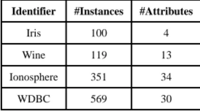
We evaluate the proposed method by clustering benchmark data sets from the UCI Archive [Asuncion and Newman. 2007]. We use four data sets with class label information, namely Iris, Wine, Ionosphere and Breast Cancer Wisconsin (Diagnostic) data sets. They are from four different domains. To make each data set contain the same number of (e.g., two) clusters, we follow the preprocessing step in [Wang and Davidson 2010] to remove the SETOSA class from the Iris data set and Class 1 from the Wine data set. The statistics of the resulting data sets are shown in Table III.

For each data set, we compute the affinity matrix using the RBF kernel [Boyd and

Vandenberghe 2004]. Our goal is to examine whether cross-domain relationship can help to enhance the accuracy of the clustering results. We construct two cross-domain relationships: Wine-Iris and Ionosphere-WDBC. The relationships are generated based on the class labels, i.e., positive (negative) instances in one domain can only be mapped to positive (negative) instances in another domain. We use the widely used Clustering Accuracy [Xu et al. 2003] to measure the quality of the clustering results. Parameter λ is set to 1 throughout the experiments. Since no existing method can handle the multi-domain co-regularized graph clustering problem, we compare our CGC method with three representative single-domain methods: symmetric NMF [Kuang et al. 2012], K-means [Späth 1985] and spectral

clustering [Ng et al. 2001]. We report the accuracy when varying the available cross-domain instance relationships (from 0 to 1 with 10% increment). The accuracy shown in Fig. 3 is averaged over 100 sets of randomly generated relationships.

We have several key observations from Fig. 3. First, CGC significantly outperforms all single-domain graph clustering methods, even though single-domain methods may perform differently on different data sets. For example, symmetric NMF works better on Wine and Iris data sets, while K-means works better on Ionosphere and WDBC data sets. Note that when the percentage of available relationships is 0, CGC degrades to symmetric NMF. CGC outperforms all alternative methods when cross-domain relationships are available. This demonstrates the effectiveness of the cross-domain relationship co-regularized method. We also notice that the performance of CGC dramatically improves when the available

relationships increase from 0 to 30%, suggesting that our method can effectively improve the clustering result even with limited information on cross-domain relationship. This is crucial for many real-life applications. Finally, we can see that RSS loss is more effective than CD loss. This is because RSS loss directly measures the weights of clustering assignment, while the CD loss does this indirectly by using linear kernel similarity first (see Section 3.1). Thus,

(18)

for a given percentage of cross-domain relationships, the method using RSS loss gains more improvements over the single-domain clustering than that using CD loss.

4.2. Robustness Evaluation

In real-life applications, both graph data and cross-domain instance relationship may contain noise. In this section, we 1) evaluate whether CGC is sensitive to the inconsistent

relationships, and 2) study the effectiveness of the relationship re-evaluation strategy proposed in Section 3.5. Due to space limitation, we only report the results on Wine-Iris data set used in the previous section. Similar results can be observed in other data sets.

We add inconsistency into matrix S with ratio r. The results are shown in Fig. 4. The percentage of available cross-domain relationships is fixed at 20%. Single-domain symmetric NMF is used as a reference method. We observe that, even when the

inconsistency ratio r is close to 50%, CGC still outperforms the single-domain symmetric NMF method. This indicates that our method is robust to noisy relationships. We also observe that, when r is very large, CD loss works better than RSS loss, although when r is small, RSS loss outperforms the CD loss (as discussed in Section 4.1). When r reaches 1, the relationship is full of noise. From the figure, we can see that CD loss is immune to noise.

In Section 3.5, we provide a method to report the cross-domain relationships that violate the single-domain clustering structure. We still use the Wine-Iris data set to evaluate its

effectiveness. As shown in Fig. 5, in the relationship matrix S, each black point represents a cross-domain relationship (all with value 1) mapping classes between the two domains. We leave the bottom right part of the matrix blank intentionally so that the inconsistent

relationships only appear between instances in cluster 1 of domain 1 and cluster 2 of domain 2. The learned confidence matrix W is shown in the figure (entries normalized to [0,1]). The smaller the value is, the stronger the evidence that the cross-domain relationship violates the original single-domain clustering structure. Reporting these suspicious relationships to users will allow them to examine the cross-domain relationships that are likely resulting from inaccurate prior knowledge.

4.3. Binary v.s. Weighted Relationship

In this section, we demonstrate that CGC can effectively incorporate weighted cross-domain relationship, which may carry richer information than binary relationship. The 20

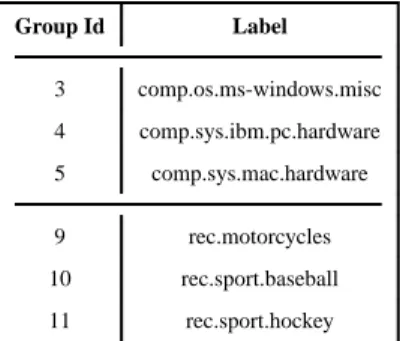
Newsgroup data set2 contains documents organized by a hierarchy of topic classes. We choose 6 groups as shown in Table IV. For example, at the top level, the 6 groups belong to two topics, computer (groups {3,4,5}) or recreation (groups {9,10,11}). The computer related data sets can be further partitioned into two subcategories, os (group 3) and sys (groups {4, 5}). Similarly, the recreation related data sets consist of subcategories motocycles (group 9) and sport (groups 10 and 11).

We generate two domains, each contains randomly sampled 300 documents from the 6 groups (50 documents from each group). To generate binary relationships, two articles are

(19)

related if they are from the same high-level topic, i.e., computer or recreation, as shown in Fig. 6(a). Weighted relationships are generated based on the topic hierarchy. Given two group labels, we compute the longest common prefix. The weight is assigned to be the ratio of the length of the common prefix over the length of the shorter of the two labels. The weighted relationship matrix is shown in Fig. 6(b). For example, if two documents come from the same group, we set the corresponding entry to 1; if one document is from rec.sport.baseball and the other from rec.sport.hockey, we set the corresponding entry to 0.67; if they do not share any label term at all, we set the entry to 0.

We perform experiments using binary and weighted relationships respectively. The affinity matrix of documents is computed based on cosine similarity. We cluster the data set into either 2 or 6 clusters and results are shown in Fig. 7. We observe that when each domain is partitioned into 2 clusters, the binary relationship outperforms the weighted one. This is because the binary relationship better represents the top-level topics, computer and recreation. On the other hand, for the domain partitioned into 6 clusters, the weighted relationship performs significantly better than the binary one. This is because weights provide more detailed information on cross-domain relationships than the binary relationships.

4.4. Evaluation of Assigning Optimal λ’s Associated with Focused Domain π

In this section, we evaluate the effectiveness of the algorithm proposed in Section 3.6 to automatically balance different cross-domain regularizers. We perform evaluation using the same setting as in Fig. 2. We have 6 different domains, each contains randomly sampled 300 documents from the 6 groups (50 documents from each group). Domain π is the one that the user focuses on. There are 5 other domains related to it. Each has randomly selected 20% available cross-domain instance relationships.

Fig. 8 shows the clustering accuracy of the 5 auxiliary domains and the focused domain π using different methods. We observed that for the focused domain π, the CGC algorithm with equal weights (λr=1/5) for regularizers outperforms the single domain clustering

(NMF). The CGC algorithm with optimal weights inferred by the algorithm in Section 3.6 outperforms the equal weights setting. This demonstrates the effectiveness of the proposed algorithm.

Fig. 9 reports the optimal weights (λr) and the corresponding clustering inconsistency μr of

each auxiliary domain when γ = 0.05. Clearly, the higher clustering inconsistency between domains r and π, the smaller weight will be assigned to r. These auxiliary domains with large μr are treated as noisy domains. In Fig. 9, only domain 1 and 4 are left when γ is 0.05.

We can further use γ to control how many auxiliary domains will be integrated for graph partition for domain π. Fig. 10 shows the optimal weights assignments when γ = 0.1 and γ = 0.15 respectively. We observed that when γ is large, all domains will be selected, i.e., each

λr will be a small but non-zero value. In contrast, when γ is small, less domains will be

(20)

4.5. Performance Evaluation

In this section, we study the performance of the proposed methods: the number of iterations before converging to a local optima and the number of runs needed to find the global optima.

Fig. 11 shows the value of the objective function with respect to the number of iterations on different data sets. We observe that the objective function value decreases steadily with more iterations. Usually, less than 100 iterations are needed before convergence. We next study the proposed population-based Tabu search algorithm for finding global optima. Using the newsgroup data sets. Fig. 12 shows the objective function values (arranged in ascending order) of 100 runs with randomly selected starting points. It can be seen that most runs converge to a global minimum. This observation is consistent with Table II. For example, according to Table II, only 4 runs are needed to find the global optima with confidence 0.999. Thus, the possibility ϕ that a random point converge to a global minimum is very high. Fig. 13 shows the number of runs used for finding global optima on various data sets. We find that only a few runs are needed to find the global optima.

4.6. Protein Module Detection by Integrating Multi-Domain Heterogenous Data

In this section, we apply the proposed method to detect protein functional modules [Hub and de G-root 2009]. The goal is to identify clusters of proteins that have strong interconnection with each other. A common approach is to cluster the protein-protein interaction (PPI) networks [Asur et al. 2007]. We show that, by integrating multi-domain heterogeneous information, such as gene co-expression network [Horvath and Dong 2008] and genetic interaction network [Cordell 2009], the performance of the detection algorithm can be dramatically improved.

We download the widely used human PPI network from BioGrid3. Three Hypertension related gene expression data sets are downloaded from Gene Expression Ominbus4 with ids GSE2559, GSE703, and GSE4737. In total, 5412 genes included in all three data sets are used to construct gene co-expression network. Pearson correlation coefficients(normalized between [0 1]) are used as the weights on edges between genes. The genetic interaction network is constructed using a large-scale Hypertension genetic data [Feng and Zhu 2010], which contains 490032 genetic markers across 4890 (1952 disease and 2938 healthy) samples. We use 1 million top-ranked genetic marker-pairs to construct the network and the test statistics are used as the weights on the edges between markers [Zhang et al. 2010]. The constructed heterogenous networks are shown in Fig. 14. The relationship between genes and genetic markers is many-to-many, since multiple genetic markers may be covered by a gene and each marker may be covered by multiple genes due to the overlapping between genes. The relationship between proteins and genes is one-to-one.

We apply CGC (with RSS loss) to cluster the generated multi-domain graphs with two different settings: (1) equal weights for each cross-domain regularizer; (2) optimal weights for each cross-domain relationship. For the first setting, we simply set weights for each cross-domain regularizer to 1. For the second setting, we consider Fig. 14 as the

(21)

combination of the two star networks. They have been shown in Fig. 15. In the first star network, genetic interaction network is the focused domain. In the second star network, PPI network is the focused domain. Then, we execute the algorithm proposed in Section 3.6 on the two star networks respectively to assign optimal λ’s. Finally, we use these optimal λ’s for clustering.

We use the standard Gene Set Enrichment Analysis (GSEA) [Mootha et al. 2003] to evaluate the significance of the inferred clusters. In particular, for each inferred cluster (protein/gene set) T, we identify the most significantly enriched Gene Ontology categories [The Gene Ontology Consortium 2000; Cheng et al. 2012]. The significance (p-value) is determined by the Fisher’s exact test. The raw p-values are further calibrated to correct for the multiple testing problem [Westfall and Young 1993]. To compute calibrated p-values for each T, we perform a randomization test, wherein we apply the same test to 1000 randomly created gene sets that have the same number of genes as T.

The calibrated p-values of the gene sets learned by CGC and single-domain graph clustering methods, symmetric NMF [Kuang et al. 2012], Markov clustering [van Dongen 2000] and spectral clustering, when applied on PPI network, are shown in Fig. 16. The clusters are arranged in ascending order of their p-values. As can be seen from the figure, by integrating three types of heterogenous networks, CGC achieves better performance than the single-domain methods. Table V shows the number of significant (calibrated p-value ≤ 0.05) modules identified by different methods. We find that CGC reports more significant

functional modules than the single-domain methods. The CGC model using optimal weights reports more significant functional modules than that using equal weights. We also apply existing multi-view graph clustering method [Kumar et al. 2011; Tang et al. 2009] on the gene co-expression networks and PPI network. Since these four networks are of the same size, multi-view method can be applied. In total, less than 20 significant modules are identified. This is because the gene expression data are very noisy. Multi-view graph clustering methods forced to find one common clustering assignment over different data sets and thus are more sensitive to noise.

5. RELATED WORK

To our best knowledge, this is the first work to study co-regularized multi-domain graph clustering with many-to-many cross-domain relationship. Existing work on multi-view graph clustering relies on a fundamental assumption that all views are with respect to the same set of instances. This set of instances have multiple representations and different views are generated from the same underlying distribution [Chaudhuri et al. 2009]. In multi-view graph clustering, research has been done to explore the most consensus clustering structure from different views [Kumar and III 2011; Kumar et al. 2011; Tang et al. 2009]. Another common approach in multi-view graph clustering is a two-step approach, which first combines multiple views into one view, then does clustering on the resulting view [Tang et al. 2012; Zhou and Burges 2007]. However, these methods do not address the many-to-many cross-domain relationship. Note that our work is different from transfer clustering [Dai et al. 2008], multi-way clustering [Banerjee et al. 2007; Bekkerman and Mccallum 2005] and

(22)

multi-task clustering [Gu et al. 2011]. These methods assume that there are some common features shared by different domains. They are also not designed for graph data.

Clustering ensemble approaches also aim to find consensus clusters from multiple data sources. Strehl and Ghosh [Strehl et al. 2002] proposed instance-based and cluster-based approaches for combining multiple partitions. Fern and Brodley [Fern and Brodley 2004] developed a hybrid bipartite graph formulation to infer ensemble clustering result. These approaches try to combine multiple clustering structures for a set of instances into a single consolidated clustering structure. Similar to multi-view graph clustering, they cannot handle many-to-many cross-domain relationships.

There are many clustering approaches based on heterogeneous information networks [Sun et al. 2009a; Sun et al. 2009b; Zhou and Liu 2013]. The problem setting of these approaches is different from ours. In our problem, the cross-domain relationships are incomplete and noisy. The clustering approaches on heterogeneous information networks typically require the complete relationships between different information networks. In addition, they can not evaluate the accuracy of the specified relationships. Moreover, our model can distinguish noisy domains and assign smaller weights to them so that the focused domain clustering can obtain optimal clustering performance.

6. CONCLUSION AND DISCUSSION

Integrating multiple data sources for graph clustering is an important problem in data mining research. Robust and flexible approaches that can incorporate multiple sources to enhance graph clustering performance are highly desirable. We develop CGC, which utilizes cross-domain relationship as co-regularizing penalty to guide the search of consensus clustering structure. By using a population-based Tabu Search, CGC can be optimized efficiently while guarantee finding the global optimum with given confidence requirement. CGC is robust even when the cross-domain relationships based on prior knowledge are noisy. Moreover, it is able to automatically identify noisy domains. By assigning smaller weights to noisy domains, the CGC algorithm is able to obtain optimal graph partition performance for the focused domain. Using various benchmark and real-life data sets, we show that the proposed CGC method can dramatically improve the graph clustering performance compared with single-domain methods.

Acknowledgments

This work is supported by the National Science Foundation, under grant XXXXXX. The authors would like to thank the reviewers and editor.

References

Asuncion A, Newman D. UCI machine learning repository. 2007; 2007

Asur, Sitaram, Ucar, Duygu, Parthasarathy, Srinivasan. An ensemble framework for clustering protein-protein interaction networks. Bioinformatics. 2007:29–40. [PubMed: 17257435]

(23)

Bekkerman, Ron, Mccallum, Andrew. Multi-way distributional clustering via pairwise interactions. ICML. 2005:41–48.

Bickel, Steffen, Scheffer, Tobias. Multi-View Clustering. ICDM. 2004:19–26.

Boyd, Stephen, Vandenberghe, Lieven. Convex Optimization. Cambridge University Press; 2004. Chaudhuri, Kamalika, Kakade, Sham M., Livescu, Karen, Sridharan, Karthik. Multi-view clustering

via canonical correlation analysis. ICML. 2009:129–136.

Cheng, Wei, Zhang, Xiang, Wu, Yubao, Yin, Xiaolin, Li, Jing, Heckerman, David, Wang, Wei. Inferring novel associations between SNP sets and gene sets in eQTL study using sparse graphical model. BCB’12. 2012:466–473.

Cordell HJ. Detecting gene-gene interactions that underlie human diseases. Nat Rev Genet. 2009; 10:392–404. [PubMed: 19434077]

Dai, Wenyuan, Yang, Qiang, Xue, Gui-Rong, Yu, Yong. Self-taught clustering. ICML. 2008:200–207. Ding, Chris, Li, Tao, Peng, Wei, Park, Haesun. Orthogonal nonnegative matrix t-factorizations for

clustering. KDD. 2006:126–135.

Dorigo, Marco, de Oca, Marco Antonio Montes, Engelbrecht, Andries Petrus. Particle swarm optimization. Scholarpedia. 2008; 3:1486.

Feng T, Zhu X. Genome-wide searching of rare genetic variants in WTCCC data. Hum Genet. 2010; 128:269–280. [PubMed: 20549515]

Fenyo, D., editor. Computational Biology. 2010. p. 327

Fern, Xiaoli Zhang, Brodley, Carla E. Solving cluster ensemble problems by bipartite graph partitioning. ICML. 2004:36–45.

Gao, Jing, Liang, Feng, Fan, Wei, Sun, Yizhou, Han, Jiawei. Graph-based Consensus Maximization among Multiple Supervised and Unsupervised Models. NIPS. 2009:585–593.

Glover, Fred, McMillan, Claude. The general employee scheduling problem. An integration of MS and AI. Computers & OR. 1986; 13:563–573.

Gu, Quanquan, Li, Zhenhui, Han, Jiawei. Learning a Kernel for Multi-Task Clustering. AAAI. 2011 Horvath, Steve, Dong, Jun. Geometric Interpretation of Gene Coexpression Network Analysis. PLoS

Computational Biology. 2008; 4

Hub, Jochen S., de Groot, Bert L. Detection of Functional Modes in Protein Dynamics. PLoS Computational Biology. 2009

Kuang, Da, Park, Haesun, Ding, Chris HQ. Symmetric Nonnegative Matrix Factorization for Graph Clustering. SDM. 2012:106–117.

Kumar, Abhishek, Daumé, Hal, III. A Co-training Approach for Multi-view Spectral Clustering. ICML. 2011:393–400.

Kumar, Abhishek, Rai, Piyush, Daumé, Hal, III. Co-regularized Multi-view Spectral Clustering. NIPS. 2011:1413–1421.

Larraanaga, Pedro, Lozano, Jose A. Estimation of Distribution Algorithms: A New Tool for Evolutionary Computation. Kluwer Academic Publishers; 2001.

Lee, Daniel D., Sebastian Seung, H. Algorithms for Non-negative Matrix Factorization. NIPS. 2000:556–562.

Leskovec, Jure, Krause, Andreas, Guestrin, Carlos, Faloutsos, Christos, VanBriesen, Jeanne M., Glance, Natalie S. Cost-effective outbreak detection in networks. KDD. 2007:420–429.

Long, Bo, Yu, Philip S., Zhang, Zhongfei (Mark). A General Model for Multiple View Unsupervised Learning. SDM. 2008:822–833.

Mootha VK, Lindgren CM, Eriksson KF, Subramanian A, Sihag S, Lehar J, Puigserver P, Carlsson E, Ridder-strale M, Laurila E, Houstis N, Daly MJ, Patterson N, Mesirov JP, Golub TR, Tamayo P, Spiegelman B, Lander ES, Hirschhorn JN, Altshuler D, Groop LC. PGC-1alpha-responsive genes involved in oxidative phosphorylation are coordinately downregulated in human diabetes. Nat Genet. 2003; 34(3):267–273. [PubMed: 12808457]

Ng, Andrew Y., Jordan, Michael I., Weiss, Yair. On Spectral Clustering: Analysis and an algorithm. NIPS. 2001:849–856.

(24)

Strehl, Alexander, Ghosh, Joydeep, Cardie, Claire. Cluster Ensembles - A Knowledge Reuse Framework for Combining Multiple Partitions. Journal of Machine Learning Research. 2002; 3:583–617.

Sun, Yizhou, Han, Jiawei. Mining Heterogeneous Information Networks: Principles and Methodologies. 2012

Sun, Yizhou, Han, Jiawei, Zhao, Peixiang, Yin, Zhijun, Cheng, Hong, Wu, Tianyi. RankClus: integrating clustering with ranking for heterogeneous information network analysis. EDBT. 2009a: 565–576.

Sun, Yizhou, Yu, Yintao, Han, Jiawei. Ranking-based clustering of heterogeneous information networks with star network schema. KDD. 2009b:797–806.

Tang, Lei, Wang, Xufei, Liu, Huan. Community detection via heterogeneous interaction analysis. Data Min Knowl Discov. 2012; 25:1–33.

Tang, Wei, Lu, Zhengdong, Dhillon, Inderjit S. Clustering with Multiple Graphs. ICDM. 2009:1016– 1021.

The Gene Ontology Consortium. Gene ontology: tool for the unification of biology. Nature Genetics. 2000; 25(1):25–29. [PubMed: 10802651]

van Dongen, Stijn. A cluster algorithm for graphs. Centrum voor Wiskunde en Informatica (CWI). 2000:40.

Wang, Xiang, Davidson, Ian. Flexible constrained spectral clustering. KDD. 2010:563–572. Westfall, PH., Young, SS. Resampling-based Multiple Testing. Wiley; New York: 1993.

Xu, Wei, Liu, Xin, Gong, Yihong. Document clustering based on non-negative matrix factorization. SIGIR (Clustering). 2003:267–273.

Yu, Guo-Xian, Rangwala, Huzefa, Domeniconi, Carlotta, Zhang, Guoji, Zhang, Zili. Protein Function Prediction by Integrating Multiple Kernels. IJCAI. 2013

Zhang X, Huang S, Zou F, Wang W. TEAM: Efficient Two-Locus Epistasis Tests in Human Genome-Wide Association Study. Bioinformatics. 2010; 26(12):i217–227. [PubMed: 20529910]

Zhou, Dengyong, Burges, Christopher JC. Spectral clustering and transductive learning with multiple views. ICML. 2007:1159–1166.

Zhou, Yang, Liu, Ling. Social influence based clustering of heterogeneous information networks. KDD. 2013:338–346.

A

uthor Man

uscr

ipt

A

uthor Man

uscr

ipt

A

uthor Man

uscr

ipt

A

uthor Man

uscr

(25)

Fig. 1.

Multi-view graph clustering vs co-regularized multi-domain graph clustering (CGC)

A

uthor Man

uscr

ipt

A

uthor Man

uscr

ipt

A

uthor Man

uscr

ipt

A

uthor Man

uscr

(26)

Fig. 2.

Focused domain i and 5 domains related to it

A

uthor Man

uscr

ipt

A

uthor Man

uscr

ipt

A

uthor Man

uscr

ipt

A

uthor Man

uscr

(27)

Fig. 3.

Clustering results on UCI datasets(Wine v.s. Iris, Ionosphere v.s. WDBC)

A

uthor Man

uscr

ipt

A

uthor Man

uscr

ipt

A

uthor Man

uscr

ipt

A

uthor Man

uscr

(28)

Fig. 4.

Clustering with inconsistent cross-domain relationship

A

uthor Man

uscr

ipt

A

uthor Man

uscr

ipt

A

uthor Man

uscr

ipt

A

uthor Man

uscr

(29)

Fig. 5.

Relationship matrix S and confidence matrix W on Wine-Iris data set)

A

uthor Man

uscr

ipt

A

uthor Man

uscr

ipt

A

uthor Man

uscr

ipt

A

uthor Man

uscr

(30)

Fig. 6.

Binary and weighted relationship matrices

A

uthor Man

uscr

ipt

A

uthor Man

uscr

ipt

A

uthor Man

uscr

ipt

A

uthor Man

uscr

(31)

Fig. 7.

Clustering results on the newsgroup data set with binary or weighted relationships

A

uthor Man

uscr

ipt

A

uthor Man

uscr

ipt

A

uthor Man

uscr

ipt

A

uthor Man

uscr

(32)

Fig. 8.

Clustering accuracy of auxiliary domains 1–5 and the focused domain π with different methods (γ = 0.05)

A

uthor Man

uscr

ipt

A

uthor Man

uscr

ipt

A

uthor Man

uscr

ipt

A

uthor Man

uscr

(33)

Fig. 9.

Optimal weights (λr) and the corresponding clustering inconsistency μr of auxiliary domain

1–5 (γ = 0.05)

A

uthor Man

uscr

ipt

A

uthor Man

uscr

ipt

A

uthor Man

uscr

ipt

A

uthor Man

uscr

(34)

Fig. 10.

Optimal weights (λr) of auxiliary domains 1–5 with different γ

A

uthor Man

uscr

ipt

A

uthor Man

uscr

ipt

A

uthor Man

uscr

ipt

A

uthor Man

uscr

(35)

Fig. 11.

Number of iterations to converge (CGC)

A

uthor Man

uscr

ipt

A

uthor Man

uscr

ipt

A

uthor Man

uscr

ipt

A

uthor Man

uscr

(36)

Fig. 12.

Objective function values of 100 runs with random initializations (newsgroup data)

A

uthor Man

uscr

ipt

A

uthor Man

uscr

ipt

A

uthor Man

uscr

ipt

A

uthor Man

uscr

(37)

Fig. 13.

Number of Runs Used for Finding Global Optima

A

uthor Man

uscr

ipt

A

uthor Man

uscr

ipt

A

uthor Man

uscr

ipt

A

uthor Man

uscr

(38)

Fig. 14.

Protein-protein interaction network, gene co-expression network, genetic interaction network and cross-domain relationships