AMBIENT NOISE TOMOGRAPHY IN NORTH-EAST UNITED STATES
Tianqi Wang
A thesis submitted to the faculty at the University of North Carolina at Chapel Hill in partial fulfillment of the requirements for the degree of Master of Science in the Department of Geological Sciences in the College
of Arts and Sciences.
Chapel Hill 2019
Approved by:
Jonathan M. Lees
Kevin G. Stewart
ABSTRACT
Tianqi Wang: Ambient Noise Tomography in North-East United States (Under the direction of Jonathan M. Lees)
The tectonic structure of the crust in the northeast region of the US is both compositionally complex and
tectonically stable relative to lithospheric structures that formed during earlier geological periods. Data from
the EarthScope Transportable Array collected in 2014 are used to calculate a three-dimensional shear velocity
model of the crust and upper mantle in the northeastern United States. We apply ambient noise tomography
and receiver function techniques to determine the Rayleigh wave phase velocities and the 3D inversion using
crustal thicknesses determined from previous body wave tomography[1]. The spatial distribution of the
structures determined by this model is well-correlated to the observed geology at the surface, including the
Atlantic Coastal Plains, the Appalachians, and New England.
The lateral distribution and depth of several slow anomalies, determined by the tomographic inversion,
within the crust of the middle Appalachians correlate with the location of Eocene volcanism. This observation
is consistent with existing tomographic models[2, 3, 4]. Since the model is highly sensitive to the crustal
thickness, higher-resolved Moho depths used in this research provide a better explanation for the material
below these volcanic structures. The tomography shows groups of slow velocities in the upper mantle in these
regions, indicating the weaker structures introduced by the Eocene volcanism.
Slow anomalies detected under the Moho discontinuity in Adirondack and New England, correlate to
the track of the Great Meteor Hotspot that passed the region approximately 100-130 Ma. Consistent with
previous research[5], this study provides evidence that the Adirondack uplift is an outcome of the Great
ACKNOWLEDGEMENTS
Throughout the writing of this dissertation, I have received a great deal of support and assistance. I
would first like to express my sincere gratitude to Dr. Jonathan Lees. As my advisor, he has lavished on
me his patience and rich knowledge from the very beginning of my study. His expertise was invaluable in
formulating my research topic and methodology in particular. His constructive advice and valuable feedback
allowed me to overcome my difficulties and progress during the writing process. Also, thousands thanks for
the trust and encouragement he has shown me throughout the past two years. I would also like to thank Dr.
Berk Biryol and Dr. Oliver Lamb for helping me working on my research. I would never be able to process
my data without the valuable experience shared by Dr. Biryol. Dr. Lamb’s advice was genuinely constructive
to my writing. Many thanks to my friends and families, whose love and support helped me putting pieces
together. Saving for the last, I would like to thank my wife, Hui Cao, for always staying by my side. Your
TABLE OF CONTENTS
LIST OF FIGURES . . . v
CHAPTER 1: INTRODUCTION . . . 1
1.1 Geologic History . . . 1
1.2 Physiographic Regions . . . 3
1.3 Ambient Noise Tomography . . . 4
CHAPTER 2: METHODS . . . 8
2.1 Data & Region Selection . . . 8
2.2 Pre-processing . . . 9
2.3 Cross-correlation . . . 9
2.4 Phase Velocity Inversion . . . 10
2.5 Shear Wave Velocity Inversion . . . 15
CHAPTER 3: RESULTS AND DISCUSSION . . . 19
3.1 Resolution . . . 19
3.2 Shear wave inversion model . . . 20
3.3 The DNAG transects cross-sections . . . 25
3.4 Discussion . . . 29
3.5 Conclusion . . . 31
LIST OF FIGURES
1.1 Map of the northeastern United States with state borders plotted. Green line is the region of this study. Red line indicates the physiographic provinces. Blue triangles are the Transportable Array seismic stations used in this study. . . 7
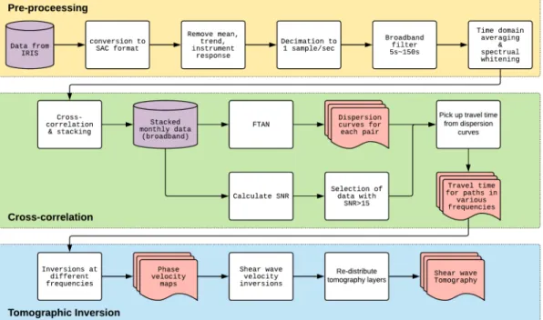
2.1 Flowchart of the Ambient Noise Tomography technique. . . 8
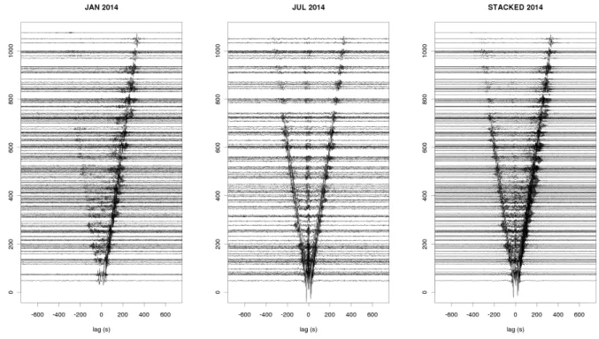
2.2 Example showing cross-correlation results of station M55A to the rest of the selected arrays. Each plot shows the cross-correlation functions in January, July, and year-round stacked in 2014. Within each plot, every horizontal line refers to one cross-correlation function between station M55A and another TA station, of which the distance from M55A is indicated on the vertical axis. Plots of January and July show a slightly different pattern, indicating a seasonal variation. The year-round stacked cross-correlation contains less noise but is still asymmetric. 10
2.3 Plot showing an example of frequency-time analysis producing the phase velocity dispersion curve of path between station M55A and V54A. The black line is the phase velocity picked from the program. . . 11
2.4 Plot showing dispersion curves from all selected station paths. The solid line is the average of the phase velocity at different frequencies. The dashed lines are the first and third quartile of the phase velocity at different frequencies. The increasing gradient of phase velocity at 25 seconds is introduced by the Mohorovičić discontinuity. . . 12
2.5 Phase velocity inversions in 15 frequencies. The two boxes on the bottom-right shows the trade-off curve of different parameters. The first box shows the results of alpha with a given sigma, and the second shows the results of sigma with a given alpha. Red dots are the model/residual size for selected alpha/sigma. . . 13
2.6 Checkerboard reconstruction test with all 15 frequencies. The first image is the input model and the rest are the reconstruction for the same parameters used in the actual inversion. Apart from the 6 seconds test, all other frequencies can reconstruct the test model well. . . 14
2.7 Crustal thickness used to constrain the model of this study. Note that the Moho depths at the coast are around 30km, while reaching 50km under the Appalachian mountains. . . 15
2.8 Averaged sensitivity kernel of this study. . . 16
2.9 Absolute shear wave velocities for the studied region. . . 17
2.10 Total misfit of the shear wave velocity model is calculated by subtracting the predicted velocity and the observed velocity at different locations. The less the misfit is, the higher the quality of the tomography is. Note that the Appalachian mountains shows apparent correspondence to high misfit values. . . 18
3.1 Path density of the phase velocity inversions. The color bar shows the numbers of paths per degree squared. Note that the 15 seconds inversion has the highest path density, while the 40 seconds inversion has the lowest path density. . . 19
3.2 Perturbations of shear wave velocities from 5 to 125 km. All depths are using the same scale, raging from -10% to 10%. . . 21
3.3 Shear velocity cross-section along the Appalachians (AA’ in Figure 3.5) . . . 24
3.4 Map of the North American continent and plate, showing positions of 19 published transects of the Centennial Continent-Ocean Transect Program. This research has referenced the E1, E3 and E4 transects. . . 26
3.6 Shear velocity cross-section of DNAG transect E-1 (BB’). . . 28
3.7 Shear velocity cross-section of DNAG transect E-3 (CC’). . . 29
CHAPTER 1
Introduction
The region of this study is the northeastern coast of the United States. This region of interest is bounded
to the north by the Canadian border, to the south by South Carolina, to the west by West Virginia and
Pennsylvania, and to the east by the US coastline. Several physiographic provinces are covered in the area,
including New England, Adirondack, Appalachian Plateau, Valley-and-Ridge Appalachians, Blue Ridge
Mountains, Piedmont and Coastal Plains. A Map of the region is shown in Figure 1.1.
The northeastern United States sits on the eastern edge of the North America continent, which has been
separated from the Pangea supercontinent since the opening of the Atlantic Ocean 170 million years ago. The
east side of the North America continent has barely gone through any tectonic events ever since. Thus, many
features that record the past two Wilson Cycles have been well-preserved in the region[6, 7, 8]. Understanding
the lithospheric structures in the region will help us learn the evolution of the continent.
Being a passive margin, the northeastern United States does not show many earthquake events. Traditional
body wave tomography can only detect deep structures, while surface wave tomography that samples the
shallower areas can be influenced by noise due to long distances from earthquake epicenters. Ambient noise
tomography, on the other hand, samples the shallower Earth with ambient surface noise. This method does
not rely on specific earthquake events; thus, it gives us the capability to research the shallower lithosphere
without the previously noted limitations.
1.1
Geologic History
Ever since the separation of the Atlantic Ocean, the northeastern United States has been free from major
tectonic activities. The relatively stable environment of this passive margin has been sustaining the ancient
crust from destruction. Thus, a wide variety of crust structures can be found in the northeast, ranging from
the late Proterozoic Grenville to the latest Atlantic sediments. The crust of this region has recorded both the
Pangea and Rodinia supercontinent cycles[9].
Based on D. W. Rankin’s summary[10], the evolution of the northeastern US started from the late
Proterozoic North America, which is part of supercontinent Rodinia. During the assembly of Rodinia, the
Grenville Orogeny formed the easternmost part of the ancient North America craton, also known as Laurentia
in some other research[11]. Seismic waves propagate in high velocity in the 1.1-billion-year old Grenville crust.
Figure 1.1: Map of the northeastern United States with state borders plotted. Green line is the region of this study. Red line indicates the physiographic provinces. Blue triangles are the Transportable Array seismic stations used in this study.
structures composed the passive margin of the Laurentia continent.
When the Iapetus Ocean closed, starting in the middle Ordovician, several orogenic processes happened
to form the Appalachian Mountains. Although the exact timing of the Appalachian Orogeny is yet to be
clarified, three major orogenic processes were introduced[10]. The Taconian Orogeny occurred from 470 to
440 Ma, forming the amalgamated Laurentia Appalachians. The amalgamated Appalachians have a high
seismic velocity. Then from 400 to 380 Ma, Laurentia collided with the Avalonia continent, and the Acadian
Orogeny formed the terranes in New England. Last, the Alleghanian Orogeny happened as Laurentia thrust
into Gondwana from 330 to 270 Ma. It was at this time that the allochthonous crust formed the accreted
seismic velocity.
After the Appalachian Orogeny, Laurentia was combined with Gondwana to form the Pangea
super-continent. It was not until the early Cenozoic that the Atlantic Ocean separated North America from the
rest of Pangea. The Atlantic passive margin consists of sediments eroded from the Appalachian Mountains.
The sediments formed a clastic wedge making up most of the coastal plain and continental shelf. Thus, the
Atlantic coast has a relatively low seismic velocity.
Although no tectonic activity happened to the northeastern United States in Cenozoic, the crust of the
area is not entirely stable. Between 46 to 47 Ma, several volcanoes erupted in the central Appalachians,
contributing to the volcanic ashes in the coastal plains of North America[12]. Later in 35 Ma, a bolide made
an impact on the east coast of Virginia, creating a crater over 40 km in diameter[13]. This impact has
deposited a large quantity of breccia to the sediments. These recent activities can lead to local low-velocity
zones in the studied region.
1.2
Physiographic Regions
In terms of its spatial distribution, the northeastern United States is categorized into seven physiographic
provinces. The placement of these physiographic provinces is connected to the geological evolution of the
North America continent.
The New England province is located in the northeastern corner of the United States. This region is
considered to result from the Acadian Orogeny. Although the crustal thickness is shallow in New England,
the dense fault zones and massive igneous intrusions indicate that it went through intense orogenic processes.
Past research[14, 15, 16] indicates the track of the Great Meteor Hotspot in the upper mantle of New England.
Adirondack is situated just west of the New England province. This province has a foundation formed
from the Grenville Orogeny, making its crust much thicker than New England. The Adirondack mountain is
known to be uplifted possibly by the same hotspot that moved past New England[5].
The Appalachian Plateau province is the highland at the west of this studied region. This province has
a deep Moho due to the Grenville crust beneath. The top of the surface, however, is covered mostly by
sedimentary rocks from the Paleozoic Era.
Both the Blue Ridge and the Valley-and-Ridge provinces are the consequences of the Appalachian Orogeny,
specifically the Alleghanian Orogeny and Taconian Orogeny[17]. These mountains have deep roots and
massive fault systems. Despite the absence of an active plate boundary, seismic and volcanic activity was still
frequent in the central Appalachians between Virginia and West Virginia in Eocene. A slow seismic upper
mantle may be related to the Cenozoic volcanism in the central Appalachians[18].
is mostly sedimentary, and its thickness is thin. Connecting the Appalachian Mountains to the coastal regions
is the Piedmont province. This province is a transitional region that has a medium crustal thickness. The
boundary between Piedmont and Coastal Plains is called the "fall line" where the elevation drops significantly.
1.3
Ambient Noise Tomography
Traditionally, seismic tomography focused on direct waves emitted from point sources such as earthquakes
and explosions. The travel time from a source to the receiver is used to invert the interior structure of the
Earth. However, this type of technique is limited by the inhomogeneous distribution of the sources. In terms
of surface wave inversions, there are several aspects that traditional tomography techniques can limit the
resolution. First, direct surface waves are not homogeneously distributed in all directions, leaving a significant
range of spaces unsampled. Second, the sources of surface waves are not always accurately located, giving
unreliable predictions of their travel paths. Third, measurements from surface waves usually cover more than
the studied area; hence, the averaged values can lower the resolution of its final product. Fourth, surface
waves can arrive at the receiver through multiple paths, making it difficult to calculate the travel time for
high-frequency waves.
Cross-correlation within a diffuse wavefield has been an alternative method to extract the Green’s function
for other fields of physics like acoustics[19]. Shapiro and Ritzwoller[20] were the first to introduce this method
in seismology, calling it ambient noise tomography. This method works with diffuse wavefields that consist of
random waves propagating in all possible directions, providing us with more information than traditional
surface wave tomography. Ambient noise tomography does not require known earthquakes but obtains the
Green’s function by cross-correlating between pairs of receivers. The following example can explain the
mathematical Green’s function deduction[21, 22].
A diffused wavefield φinside an elastic body (such as the Earth) can be expressed by:
φ(x, t) =X
n
anun(x)eiωnt (1.1)
Wherexis position,tis time,un andωn are eigenfunctions and eigenfrequencies of the Earth, andanare
modal excitation functions. The modal amplitudes are uncorrelated random variables:
hana∗mi=δnmF(ωn) (1.2)
where F(ωn)is the spectral energy density. According to equation(1.2), the cross-terms will cancel out
C(x, y, τ) =hφ(x, t)φ(y, t+τ)i=X
n
F(ωn)un(x)un(y) cos (ωnτ) (1.3)
Where τ is the lag of the correlation. When F(ωn) is a constant and τ is positive, this function is
equivalent to the Green’s function of waves propagating fromxtoy:
G(x,y, τ) =X
n
un(x)un(y) cos (ωnτ)
(τ >0,0, otherwise)
(1.4)
Note that euqations (1.3) and(1.4)differ only in the amplitude factor F(ωn)and the negativeτ term.
Thus, with the cross-correlation between a pair of receivers, the travel time of the diffused surface waves can
be extracted. Hence:
C(x, y, τ) =F(ωn) [G(x,y, τ) +G(x,y,−τ)] (1.5)
In the past few years, ambient noise tomography has been applied in numerous regions, including western
North America[23, 24, 25], South America[26], Europe[27], and Australia[28, 29]. These studies have produced
high-resolution tomography inversions up to 200 km depth. As for the northeastern United States, where
several tomography was produced[30, 31, 4], the quality at shallower depths is not well-resolved. Ambient
CHAPTER 2
Methods
Figure 2.1: Flowchart of the Ambient Noise Tomography technique.
2.1
Data & Region Selection
The flowchart of this research, based on Bensen’s guide to ambient noise tomography[32, 33], is summarized
in Figure 2.1. Contrary to body wave and surface wave inversions, this method does not require a known set
of earthquake events. The data we need for this research is just the record of a vast seismic network. In order
to reduce the inconsistency of wave sources, an extended time of recording is preferred.
The EarthScope project has deployed massive seismic networks in the United States, including the
Transportable Array (TA)[34]. This study collected the data from 221 TA stations throughout the year of
2014 (blue triangles in Figure 1.1). Most of the stations have the full record over the year, while a few stations
only have partial records. All TA stations in this research use the same seismic instrument. The signal has
has a sample rate of 40 samples per second.
2.2
Pre-processing
Before cross-correlating the records at each station, they need to be downsampled and bandpass filtered at
5 to 150 seconds. Since the shortest wavelength used in this study is 6 seconds, a sampling rate of 1 sample
per second will be abundant to satisfy the Nyquist sampling criterion. As we want the cross-correlation of the
ambient noise, we need to remove the impact of major earthquake events. The 5 to 150 bandpass filter can
remove earthquake signals at higher frequencies. Then, a running-absolute-mean normalization was applied
to remove earthquakes in lower frequencies. In addition to time domain averaging, spectrum whitening was
applied in the frequency domain.
Figure 2.2: Example showing cross-correlation results of station M55A to the rest of the selected arrays. Each plot shows the cross-correlation functions in January, July, and year-round stacked in 2014. Within each plot, every horizontal line refers to one cross-correlation function between station M55A and another TA station, of which the distance from M55A is indicated on the vertical axis. Plots of January and July show a slightly different pattern, indicating a seasonal variation. The year-round stacked cross-correlation contains less noise but is still asymmetric.
2.3
Cross-correlation
Cross-correlation was done in three steps. First, we calculate the daily cross-correlation with 221 stations,
making 24,310 cross-correlation paths. For stations with incomplete data, we only calculate the results when
cross-correlation results of one path can vary between months due to the seasonal source of ambient noise.
Lastly, to remove the influence of seasonal variation, the monthly results are combined with a weighting
parameter that averaged out significant high amplitudes.
The final product of the cross-correlation was 24,310 cross-correlation functions over the stacked 24-hour
time window. Given the station network’s geometry limits the maximum travel time being 500 seconds, the
time windows of the records were cut down to 1000 seconds for better storage management. An example of
the cross-correlation results is given in Figure 2.2.
Each cross-correlation function should have two windows showing the positive and the negative Green’s
function of the path. In theory, both windows should have the same amplitudes. However, due to the
inhomogeneous distribution of the sources of ambient noise, the year-round stacked results are not symmetric.
To reduce the bias introduced by the sources, we took the symmetric results by averaging the positive and
negative windows.
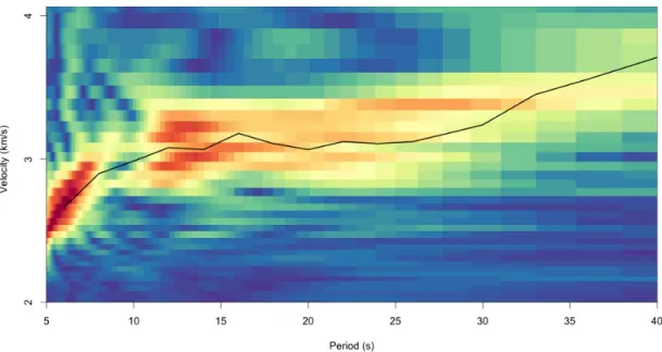
Figure 2.3: Plot showing an example of frequency-time analysis producing the phase velocity dispersion curve of path between station M55A and V54A. The black line is the phase velocity picked from the program.
2.4
Phase Velocity Inversion
Surface waves of different frequencies propagate at different velocities. This property of surface waves
is called dispersion. In order to know how fast each frequency travels in one path, we applied FTAN
Figure 2.4: Plot showing dispersion curves from all selected station paths. The solid line is the average of the phase velocity at different frequencies. The dashed lines are the first and third quartile of the phase velocity at different frequencies. The increasing gradient of phase velocity at 25 seconds is introduced by the Mohorovičić discontinuity.
faster inversion[33]. Figure 2.3 gives an example of how FTAN obtains the dispersion curve with one pair
of stations. While some station paths can have poor signals at a specific frequency, we also output the
signal-to-noise ratio (SNR) together with the dispersion curve as an evaluation of the FTAN quality.
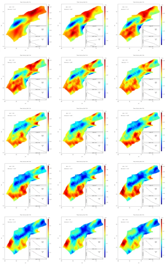
In this study, we picked 15 frequencies from the dispersion curves to invert for phase velocity maps,
ranging from 6 to 40 seconds. Before the phase velocity inversion, we removed the paths that have an SNR
less than 15. All phase velocity inversions were done through two steps of iterations. The first step used all
provided paths to produce a preliminary model. After rejecting paths with significant discrepancies from the
model prediction, a second inversion produced the final result. The model of this study covers a latitude
from 30N to 48N, a longitude from 67W to 85W, with a resolution of 0.1 degrees.
Two parameters control the results of the inversion program: damping (alpha) and sensitivity radius
(sigma). While the radius parameter had little effect on the inversion results, damping played a vital role in
the quality of the inversion. While the prediction residuals remained comparably small, the size of the model
shrank drastically with increasing damping. After comparing the inversions with previous studies[35, 1, 4]
all phase velocity inversions. The parameters were meant to be kept the same for all frequencies to avoid
additional bias when interpreting the models. The phase velocity inversion results are shown in Figure 2.5.
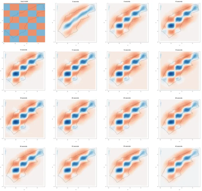
Following the inversions, we tested the phase velocity model with an artificial checkered board. Figure
2.6 shows the results of the checkered board test. Apart from the 6-second phase velocity model, all tested
models can reconstruct the checkered board well. The short-period model, however, showed a strong smearing
effect due to the poor SNR at this frequency. Among 24,310 paths calculated in this study, only less than
9,000 paths satisfied the SNR requirement.
2.5
Shear Wave Velocity Inversion
Figure 2.7: Crustal thickness used to constrain the model of this study. Note that the Moho depths at the coast are around 30km, while reaching 50km under the Appalachian mountains.
The inhomogeneous structures govern surface wave dispersion in the crust and upper mantle. Thus, we
Figure 2.8: Averaged sensitivity kernel of this study.
tomography is produced by combining all frequencies with a corresponding sensitivity kernel[36]. The shear
wave inversion requires a starting model, which is modified based on the IASPEI and the CRUST 2.0 earth
model. The modification is done by reassigning the velocity layers based on the Moho discontinuity from a
recent study (Figure 2.7)[1]. We did 50 iterations of linear inversion at each location within a 180 by 180 grid.
The inversion results converged far before the 50th iteration, and the sensitivity kernels (Figure 2.8) are close
to previous research in North America[33, 35, 4].
However, since the crustal thickness of the studied region changes dramatically, the absolute shear wave
velocity was dominated by the changing Moho depths. The initial model (Figure 2.9) had difficulty in
inverting areas where the Moho changes abruptly. According to the misfit shown in Figure 2.10, we can tell
that the misfit is generally higher along the Appalachian Mountains, where we encounter a higher gradient of
the Moho depths. In order to resolve minor structures, we calculated shear wave perturbations in 24 layers, 7
of which are above the Moho Discontinuity. The shear wave perturbation maps are shown in depths up to
150km. By removing the impact of the Moho, more detailed structures around 30 to 50 km can be revealed.
CHAPTER 3
Results and discussion
3.1
Resolution
Resolution of the inversion depends on two factors: the phase velocity resolution and the sensitivity
kernels. The phase velocity inversion controls the resolution in the spatial dimension. The resolution of phase
velocity maps decreases as the density of paths decreases. Figure 3.1 shows the path density of phase velocity
inversion at 6, 15, 25, and 35 seconds.
Figure 3.1: Path density of the phase velocity inversions. The color bar shows the numbers of paths per degree squared. Note that the 15 seconds inversion has the highest path density, while the 40 seconds inversion has the lowest path density.
One of the major factors that biases the phase velocity inversion is the source distribution. The
fundamentals of ambient noise tomography include the assumption of a homogeneous wavefield. However,
several locations generate stronger signals than the rest of the world. Research[37] has shown microseisms
generated by ocean current in northern Atlantic and eastern Pacific. Although we stacked our data to reduce
seasonal variations, the noise level at certain stations remains high.
At higher frequencies (periods shorter than 10 seconds), many stations are contaminated by high noise
levels, and their SNR is below the threshold. As a result, we had to reject more than 10,000 paths to keep
reasonable confidence in the inversion. Most of the rejected paths are in the lateral direction, causing a strong
smearing effect on the phase velocity result. The checkered board test in Figure 2.6 also shows that the 6
seconds results smear along the Appalachian Mountains.
At lower frequencies (periods longer than 30 seconds), where a full wavelength passes a distance over
paths were rejected during the cross-correlation at 40 seconds. Similar to that of high frequencies, the phase
velocity inversion of low frequencies also suffers from smearing effects.
The sensitivity kernels explain the coverage of different frequencies in the vertical dimension. Shorter
periods are sensitive at shallower depths, but more constrained within their sensitivity range. Longer periods
are sensitive to deeper depths but span a lot wider with their sensible range. Thus, the resolution of the
model reduces as the depth increases. Combined with the resolution at each frequency, the resolution for this
study is best at depth from 10 to 60 km, while not very good for near-surface lithosphere and deeper in the
mantle.
3.2
Shear wave inversion model
This 3-D model describes the crust and upper mantle structure in the eastern United States. The result
of the inversion is the shear wave velocity perturbation at depths up to 125 km. The influence of the Moho
Discontinuity has been removed; thus, the final model does not show the difference between the crust and the
mantle (Figure 3.2).
Depths less than 25 km are all above the Moho discontinuity. Although the depths of sediments are usually
less than 5 km in the studied region, some information of the sediments can pass to deeper tomography due
to surface wave dispersion. At these depths, we see two high-velocity zones and four low-velocity zones. The
two high-velocity zones are located at northern and southern Appalachians, and the low-velocity zones are
located at Coastal Plains, Appalachian Plateaus, and eastern New England.
The high-velocity zones in both northern and southern Appalachians correspond to the igneous and
metamorphic bedrock on the surface. However, there is a discontinuity of high velocity in Pennsylvania.
This might be the smearing effect of high-frequency inversions. The high-velocity zone in the northern
Appalachians covers the whole Adirondack province, correlating to the thick metamorphosed shield seen in
previous research[5]. Some minor low-velocity zones start to appear near the Moho discontinuity, which can
result from the intrusions in the area[38]. The high-velocity zone in the southern Appalachians extends to the
southern coast of North Carolina, near the location of the Cape Fear Arch, which does not agree with other
research[35, 3]. Since two low-velocity zones surround this area in Coastal Plain, the high velocity we see on
the map might be the fact that the two other low-velocity zones are even slower than the coastline sediments.
There is a sizable low-velocity zone between Pennsylvania and West Virginia. This slow area relates to
the sedimentary basin in Appalachian Plateau. Another two low-velocity zones appear in Coastal Plain, one
in Virginia and the other in South Carolina. The location of the Virginia low-velocity zone relates to the
Chesapeake Bay impact crater[13]. Although the size of the crater is much smaller than the low-velocity
theory explaining the large low-velocity zone is the geometry of the continent. When propagating offshore of
Virginia, seismic waves pass through longer distances on the ocean floor. Thus, the velocity in this model
appears to be slower along the Virginia coast. The low-velocity zone in South Carolina locates near the
Charleston Seismic Zone, also known as the Middleton Place Summerville Seismic Zone. Previous research[4]
shows a larger area of this slowness, but this study can confine it onto the faults of this seismic zone. The last
low-velocity zone is in eastern New England, in the state of Maine. Past research[5] shows a similar slowness
near the surface, but the explanation is yet to be stated.
Between the depth of 30 and 50 km is the Moho discontinuity, where the resolution is at a maximum.
The Moho model that we used to produce the tomography does not resolve detailed structures. We used a
smoothened Moho as we do not want it to dominant results at depths between 30 and 50 km. The Moho is
shallow along the coast, ranging around 30 km. Its depth increases drastically under the Appalachians. At
the westernmost of this studied region, the Moho depth is at its maximum of 50 km.
The two high-velocity zones are subject to minor changes. The high-velocity zone in Adirondack disappears
at the Moho boundary and changes into a low-velocity zone. The sub-Moho Adirondack low-velocity zone
connects to some other slow regions in southern New England. Earlier research[5] suggests this being the
uplift caused by the Great Meteor Hotspot. The high-velocity zone in the southern Appalachians dies out as
depth increases. On the other hand, a large high-velocity zone appears at the easternmost of the studied
region, corresponding to the location of the Grenville foundation[39].
Two of the low-velocity zones in the shallower layers show changes near the Moho boundary. The
low-velocity zone in coastal Virginia disappears, agreeing to the fact that the Chesapeake Bay impact crater
is shallow in the crust. The low-velocity zone between Pennsylvania and West Virginia changes its location
to the east, beneath the Appalachian ridges. The lower velocity under the Appalachian Orogeny can be the
roots of the mountains[9]. Both the low-velocity zones in South Carolina and Maine remain at the same
location. The low velocity in South Carolina indicates that the weak structure under the Middleton Place
Summerville Seismic Zone continues even below the Moho, providing evidence for the cause of the seismicity.
The low-velocity zone in Maine can be due to the thinner Avalonian crust, but the high perturbation is hard
to explain with the surface geology.
From the Moho Discontinuity to the depth of 100 km, we start to see a slow anomaly appearing at the
east edge of West Virginia. Other research[3] has also observed this low-velocity zone. This location correlates
to the appearance of Eocene volcanism, and the anomalies can be explained as the delamination underneath
the volcanos[16]. The low velocity beneath Adirondack is connected to the lower regions in the west of
Massachusetts and Connecticut. The specific location of the hotspot is hard to locate as its materials spread
robust structure under the Grenville crust.
Below 100 km depth, the resolution of the inversion is reduced, and the structures at deeper layers are
very similar to what is above them, mostly due to the wide sensitivity kernels of the longer periods in phase
velocity inversions.
Figure 3.3: Shear velocity cross-section along the Appalachians (AA’ in Figure 3.5)
A cross-section of the model is made along the Appalachian Mountains (Figure 3.3). The Moho depth
of this cross-section stays constant at around 40 km. The high-velocity zone under Adirondack shows the
thick Grenville shield. The slow anomaly under the presumed Great Meteor Hotspot is substantial evidence
showing the weaker material introduced by the hotspot. We see some low-velocity zones under Maine, on
either side of the Moho, but the theory for this observation is unclear at the moment. There is a continuous
low-velocity zone under the Valley and Ridge and Appalachian Plateau province. This can be the synergy of
the fault zones and sediments in the region. Some slower anomalies appear under the Moho boundary at the
location of the Eocene volcanism (yellow triangles in Figure 3.3), indicating the unstable structures under the
Eocene volcanoes.
3.3
The DNAG transects cross-sections
The Geological Society of America established the Decade of North American Geology (DNAG) Project
including the Northeastern United States. Within its Continent-Ocean Transects volume, several studies
have discussed the crustal and upper mantle geology. The E1 transects covered the Adirondacks to Georges
Bank[41]. The E3 transects covered southwestern Pennsylvania to the Baltimore Canyon Trough[42]. The E4
transects covered Central Kentucky to Carolina Trough[43]. These materials provide us with an excellent
background to interpret the tomography results. In addition to the Appalachian cross-section (AA’), we made
three other cross-sections (BB’, CC’ and DD’) at the locations of the E1, E3, and E4 transect. To compare
the tomography to the DNAG transects, we extracted the crustal structures from each of the transects and
plotted them on top of the cross-sections. Note that the Moho used in this study does not necessarily agree
to the Moho in the DNAG studies. The Moho in this study is smooth and might lose some details.
Transect E1 (Figure 3.6) shows the velocity transition in Adirondack and New England. There is a definite
shift from fast to slow in the State of New York and Vermont. The velocity difference also correlates to the
crustal geologic history, that the Grenville crust is faster than the Avalonian crust. The slow anomalies under
the Moho boundary could be the Great Meteor Hotspot that moved through the Adirondack shield, causing
uplift in the region. There is also one slow anomaly above the Moho in this cross-section, which may be
related to the transition zone in the crust.
Transects E3 (Figure 3.7) also shows the Grenville crust as a high-velocity. The Coastal Plain has a slower
velocity in the crust, as a result of the loose sediments and the impact crater in the Chesapeake Bay. Some
fast velocities appear near Moho under the Taconian structure. These high-velocity zones can be the result
of the subduction of Grenville into the Taconian crust. The Eocene volcanism (yellow triangles in Figure
3.7) shows a significantly different pattern under the Moho boundary, even though it is positioned in the
Grenville crust. The sub-Moho slowness is clear proof that the upper mantle under the volcano is relatively
more active than the surrounding areas[3, 2]. The Appalachian Plateaus province at the western edge is
showing a slower velocity in the crust due to its low-velocity sedimentary basin.
Transect E4 (Figure 3.8) is a generally faster cross-section. At its westernmost, the high-velocity zones
correspond to the position of the Grenville Front. The fast and shallow crust in the Piedmont province can
be related to the igneous intrusions above the Laurentia basement. The Taconian accretion in the coastal
plains is relatively slower than the Piedmont crust in the inland. However, there is a fast anomaly right at the
Moho boundary in Coastal Plains, which could be an artifact introduced by an erroneous Moho input when
inverting the shear wave velocities. The DNAG studies indicate some plutonic intrusions in the Coastal Plain.
Figure 3.6: Shear velocity cross-section of DNAG transect E-1 (BB’).
Figure 3.8: Shear velocity cross-section of DNAG transect E-4 (DD’).
3.4
Discussion
Because the cross-correlation results are influenced by seasonal variations, taking an unweighted average
of the cross-correlation results cannot remove the bias introduced by sources such as the Atlantic microseism.
It will be more reliable if we can analyze the location of the sources and rearrange the weights to annihilate
the biases.
The Appalachian orogeny has gone through multiple collisions. As a result, the complex folding and faults
along the mountains have introduced anisotropy in the crust. Without analyzing the anisotropy in further
details, this study tried to remove the impact of the anisotropy with a strong damping parameter. However,
the damping would not necessarily remove all anisotropy and thus causing a high misfit of the inversion,
making the final model less reliable. Besides, the anisotropy generated by fault zones forces the program to
reject many cross-correlation paths, reducing the path density and the resolution.
In the inversions of this study, we always use a staring model and apply multiple iterations of inversion to
produce the results. However, the inversions do not always converge to the same results, and the quality
of the results is highly dependent on the starting model. Although we have adjusted the starting models
to fit the geologic backgrounds, there is the possibility that we have overlooked some details. Some other
also helps to produce better statistics about tomography quality.
In comparison to the continental scale inversions, this study provides better resolution by constraining
the area size. However, the studied region is still too large to produce tomography for detailed geological
research. It will be easier for us to differentiate geologic features in more details if the size of the studied
region is further refined. Moreover, more stations outside of the studied region can be helpful to reduce the
edge effects of ambient noise cross-correlations.
3.5
Conclusion
The tectonic structure of the crust in the northeast region of the United States is both compositionally
complex and tectonically stable relative to lithospheric structures that formed during earlier geological periods.
Data from the EarthScope Transportable Array collected in 2014 are used to calculate a three-dimensional
shear velocity model of the crust and upper mantle in the northeastern United States. We apply ambient noise
tomography to determine the Rayleigh wave phase velocities and the 3D inversion using crustal thicknesses
of the conterminous United States[1]. In general, the spatial distribution of the structures determined by this
model is well-correlated to the observed geology at the surface, including the coastal sedimentary regions, the
Appalachian orogeny, and the New England area.
The lateral distribution and depth of several slow anomalies, determined by the tomographic inversion,
within the crust of the central Appalachians correlate to Eocene volcanism. This observation is consistent with
past tomographic models[2, 3, 4]. Since the model is highly sensitive to the crustal thickness, higher-resolved
Moho depths used in this research provide a better explanation for the material below these volcanic structures.
The tomography shows groups of fast velocities in the upper mantle in these regions, indicating the presence
of denser materials that have been supporting the gradual volcanism since the Eocene.
A fast anomaly detected in the inversion, close to the surface of the New England crust, correlates with
the igneous intrusions generated by the Great Meteor Hotspot, which formed approximately 100-130 Ma.
The tomography produced by this study also shows the connection between the hotspot and the Adirondack
uplift, agreeing to previous observations of the hotspot[5].
We have observed two low-velocity zones in the Atlantic Coastal Plain. The low-velocity zone in the
Chesapeake Bay provides evidence of the deeper influence of the bolide impact. The low-velocity zone in
South Carolina can help us understand the cause of the Charleston seismicity. We have also observed a
low-velocity zone in Maine; however, we are unable to come to a robust conclusion on this observation.
REFERENCES
[1] B. Schmandt and F. Lin, “P and S wave tomography of the mantle beneath the United States,”Geophysical Research Letters, vol. 41, pp. 6342–6349, 2014.
[2] R. Porter, Y. Liu, and W. E. Holt, “Lithospheric records of orogeny within the continental U.S.,”
Geophysical Research Letters, vol. 43, pp. 144–153, 2016.
[3] L. S. Wagner, K. M. Fischer, R. Hawman, E. Hopper, and D. Howell, “The relative roles of inheritance and long-term passive margin lithospheric evolution on the modern structure and tectonic activity in the southeastern United States,” Geosphere, 2018.
[4] C. B. Biryol, L. S. Wagner, K. M. Fischer, and R. B. Hawman, “Relationship between observed upper mantle structures and recent tectonic activity across the Southeastern United States,” Journal of Geophysical Research: Solid Earth, vol. 121, pp. 3393–3414, 2016.
[5] X. Yang and H. Gao, “Full-wave seismic tomography in the northeastern united states: New insights into the uplift mechanism of the adirondack mountains,”Geophysical Research Letters, vol. 45, pp. 5992–6000, 6 2018.
[6] W. A. Thomas, “Tectonic inheritance at a continental margin,” GSA Today, vol. 16, p. 4, 2006.
[7] R. Russo and P. Silver, “Cordillera formation, mantle dynamics, and the wilson cycle,” Geology, vol. 24, no. 6, pp. 511–514, 1996.
[8] R. Evans, “Anisotropy: a pervasive feature of fault zones?,” Geophysical Journal International, vol. 76, pp. 157–163, 01 1984.
[9] K. E. Karlstrom, K.-I. Åhäll, S. S. Harlan, M. L. Williams, J. McLelland, and J. W. Geissman, “Long-lived (1.8–1.0 Ga) convergent orogen in southern Laurentia, its extensions to Australia and Baltica, and
implications for refining Rodinia,” Precambrian Research, vol. 111, pp. 5–30, 2001.
[10] D. W. Rankin, “Appalachian salients and recesses: Late Precambrian continental breakup and the opening of the Iapetus Ocean,” Journal of Geophysical Research, vol. 81, pp. 5605–5619, 1976.
[11] J. Hibbard, “Docking Carolina: Mid-Paleozoic accretion in the southern Appalachians,” Geology, vol. 28, pp. 127–130, 2000.
[12] P. D. Fullagar and M. L. Bottino, “Tertiary felsite intrusions in the valley and ridge province, virginia,”
Geological Society of America Bulletin, vol. 80, no. 9, pp. 1853–1858, 1969.
[13] G. S. Collins and K. Wunnemann, “How big was the chesapeake bay impact? insight from numerical modeling,” Geology, vol. 33, no. 12, pp. 925–928, 2005.
[14] V. Levin, M. D. Long, P. Skryzalin, Y. Li, and I. López, “Seismic evidence for a recently formed mantle upwelling beneath New England,” Geology, vol. 46, pp. 87–90, 2018.
[15] W. Menke, P. Skryzalin, V. Levin, T. Harper, F. Darbyshire, and T. Dong, “The Northern Appalachian Anomaly: A modern asthenospheric upwelling,” Geophysical Research Letters, vol. 43, 2016.
[16] S. E. Mazza, E. Gazel, E. A. Johnson, M. J. Kunk, R. McAleer, J. A. Spotila, M. Bizimis, and D. S. Coleman, “Volcanoes of the passive margin: The youngest magmatic event in eastern North America,”
Geology, vol. 42, pp. 483–486, 2014.
[18] E. H. Parker, R. B. Hawman, K. M. Fischer, and L. S. Wagner, “Crustal evolution across the southern Appalachians: Initial results from the SESAME broadband array,” Geophysical Research Letters, vol. 40, pp. 3853–3857, 2013.
[19] O. I. Lobkis and R. L. Weaver, “On the emergence of the Green’s function in the correlations of a diffuse field,”The Journal of the Acoustical Society of America, vol. 110, pp. 3011–3017, 2001.
[20] N. M. Shapiro and M. Campillo, “Emergence of broadband Rayleigh waves from correlations of the ambient seismic noise,” Geophysical Research Letters, vol. 31, 2004.
[21] R. Snieder, “Extracting the Green’s function from the correlation of coda waves: A derivation based on stationary phase,” Physical Review E, vol. 69, p. 046610, 2004.
[22] R. Snieder and K. Wapenaar, “Imaging with ambient noise,” Physics Today, vol. 63, pp. 44–49, 2010.
[23] N. M. Shapiro, M. Campillo, L. Stehly, and M. H. Ritzwoller, “High-Resolution Surface-Wave Tomography from Ambient Seismic Noise,” Science, vol. 307, 2005.
[24] F.-C. Lin, D. Li, R. W. Clayton, and D. Hollis, “High-resolution 3D shallow crustal structure in Long Beach, California: Application of ambient noise tomography on a dense seismic arrayNoise tomography with a dense array,” Geophysics, vol. 78, pp. Q45–Q56, 2013.
[25] C. Chai, C. J. Ammon, M. Maceira, and R. B. Herrmann, “Inverting interpolated receiver functions with surface wave dispersion and gravity: Application to the western U.S. and adjacent Canada and Mexico,”
Geophysical Research Letters, vol. 42, pp. 4359–4366, 2015.
[26] J. R. Delph, K. M. Ward, G. Zandt, M. N. Ducea, and S. L. Beck, “Imaging a magma plumbing system from MASH zone to magma reservoir,” Earth and Planetary Science Letters, vol. 457, 2017.
[27] Y. Yang, M. H. Ritzwoller, A. L. Levshin, and N. M. Shapiro, “Ambient noise Rayleigh wave tomography across Europe,” Geophysical Journal International, vol. 168, pp. 259–274, 2007.
[28] E. Saygin and B. L. Kennett, “Ambient seismic noise tomography of Australian continent,”Tectonophysics, vol. 481, pp. 116–125, 2010.
[29] P. Arroucau, N. Rawlinson, and M. Sambridge, “New insight into Cainozoic sedimentary basins and Palaeozoic suture zones in southeast Australia from ambient noise surface wave tomography,”Geophysical Research Letters, vol. 37, 2010.
[30] L. S. Wagner, M. J. Fouch, D. E. James, and S. Hanson-Hedgecock, “Crust and upper mantle structure beneath the Pacific Northwest from joint inversions of ambient noise and earthquake data,”Geochemistry, Geophysics, Geosystems, vol. 13, 2012.
[31] W. Shen and M. H. Ritzwoller, “Crustal and uppermost mantle structure beneath the United States,”
Journal of Geophysical Research: Solid Earth, vol. 121, pp. 4306–4342, 2016.
[32] G. D. Bensen, M. H. Ritzwoller, M. P. Barmin, A. L. Levshin, F. Lin, M. P. Moschetti, N. M. Shapiro, and Y. Yang, “Processing seismic ambient noise data to obtain reliable broad-band surface wave dispersion measurements,” Geophysical Journal International, vol. 169, pp. 1239–1260, 2007.
[33] G. D. Bensen, M. H. Ritzwoller, and N. M. Shapiro, “Broadband ambient noise surface wave tomography across the United States,” Journal of Geophysical Research: Solid Earth (1978–2012), vol. 113, 2008.
[34] M. Williams, K. M. Fischer, J. T. Freymueller, B. Tikoff, A. M.Tréhu,et al., “Unlocking the secrets of the north american continent: An earthscope science plan for 2010-2020,” www.earthscope.org, p. 78, February 2010.
[36] M. Saito, “DISPER80: A subroutine package for the calculation of seismic normal-mode solutions,”
Seismological algorithms, 1988.
[37] S. Kedar, M. Longuet-Higgins, F. Webb, N. Graham, R. Clayton, and C. Jones, “The origin of deep ocean microseisms in the North Atlantic Ocean,” Proceedings of the Royal Society A: Mathematical, Physical and Engineering Sciences, vol. 464, pp. 777–793, 2008.
[38] K. A. Foland and J. C. Allen, “Magma sources for Mesozoic anorogenic granites of the White Mountain magma series, New England, USA,” Contributions to Mineralogy and Petrology, vol. 109, pp. 195–211, 1991.
[39] C. A. Stein, “Is the “Grenville Front” in the central United States really the Midcontinent Rift?,” GSA Today, 2017.
[40] P. Hoffman, “The geology of north america—an overview,” 1989.
[41] J. B. Thompson and R. C. Speed, Centennial Continent/ocean Transect# 17: E-1 Adirondacks to Georges Bank. Geological Society of America, 1993.
[42] L. Glover and K. D. Klitgord,E-3 southwestern Pennsylvania to Baltimore Canyon Trough. Geological Society of America, 1995.
[43] D. Rankin,North American Continent-ocean Transect E-4: Central Kentucky to the Carolina Trough. Geological Society of America, 1991.