Complex Systems Informatics and Modeling Quarterly
CSIMQ, Article 68, Issue 12, September/October 2017, Pages 1–21 Published online by RTU Press, https://csimq-journals.rtu.lv https://doi.org/10.7250/csimq.2017-12.01
ISSN: 2255-9922 online
Human Performance-Aware Scheduling and Routing of a
Multi-Skilled Workforce
Maikel L. van Eck1??, Murat Firat1?, Wim P. M. Nuijten1,2?,
Natalia Sidorova1?, and Wil M. P. van der Aalst1?
1Eindhoven University of Technology, The Netherlands 2Quintiq, Utopialaan 25, ‘s-Hertogenbosch, The Netherlands
{m.l.v.eck,m.firat,w.p.m.nuijten,n.sidorova,w.m.p.v.d.aalst}@tue.nl
Abstract. Planning human activities within business processes often happens based on the same methods and algorithms as are used in the area of manufacturing systems. However, human behaviour is quite different from machine behaviour. Their performance depends on a number of factors, including workload, stress, personal preferences, etc. In this article we describe an approach for scheduling activities of people that takes into account business rules and dynamic human performance in order to optimise the schedule. We formally describe the scheduling problem we address and discuss how it can be constructed from inputs in the form of business process models and performance measurements. Finally, we discuss and evaluate an implementation for our planning approach to show the impact of considering dynamic human performance in scheduling.
Keywords: Scheduling, business process management, dynamic human performance, mixed integer programming.
1
Introduction
Scheduling is used in the planning of personnel and human activities in different environments [1], [2], [3]. Traditionally, scheduling problems are often presented as optimisation problems in the context of manufacturing systems, where a set of jobs is to be assigned to a set of machines such that the total length of the schedule is minimized. However, the basic job shop scheduling problem has been extended and scheduling problems now exist in many different variations and settings, each with their own characteristics. These variations aim to incorporate the complexity of the real world in order to increase the applicability of their solutions, but this generally increases the difficulty of finding an optimal schedule.
??This research was performed in the context of the IMPULS collaboration project of Eindhoven University of Technology and
Philips: “Mine your own body”.
? Corresponding authors
c
2017 Maikel L. van Eck et al. This is an open access article licensed under the Creative Commons Attribution License (http://creativecommons.org/licenses/by/4.0).
Reference: M. L. van Eck, M. Firat, W. P. M. Nuijten, N. Sidorova, and W. M. P. van der Aalst, “Human Performance-Aware Scheduling and Routing of a Multi-Skilled Workforce,” Complex Systems Informatics and Modeling Quarterly, CSIMQ, Issue no. 12, pp. 1–21, 2017. Available: https://doi.org/10.7250/csimq.2017-12.01
Nowadays, the work in many organisations such as hospitals and financial institutions is done according to predefined business processes [4], [5]. These processes specify which activities need to be executed, in what order and by whom [6], [7]. The field of Business Process Management (BPM) can be defined as a discipline involving modeling, automation, execution, control, measurement and optimization of these business activity flows. Therefore, we are interested in incorporating elements from BPM, such as the use of process models, into human activity scheduling in order to match the current way of working.
Additionally, in the majority of scheduling literature, activity or job durations are assumed to be fixed [1], [2], [3]. In reality job durations may vary due to uncertainties in the nature of the process such as machine breakdown and accidents, but also due to variations in human performance. People’s performance changes dynamically depending on factors such as their experience, stress and workload [8], [9], [10], [11]. This means that the schedule itself, including the number of breaks and the order of jobs performed, affects human performance and therefore the realisations of job durations. Hence, we argue that the accuracy of schedules and the timely execution of processes can be improved by taking a dynamic view of human performance.
In order to take dynamic human performance into account during scheduling, we need to establish the interactions between performance and the execution of the activities to be scheduled. Part of this information can be gathered by logging the jobs being performed by people and their duration. Other information such as the relation between stress and performance can be obtained using new technological advances and smart sensor technologies [12], [13]. These enable unobtrusive monitoring of personal stress levels to identify sources of stress at work and discover performance patterns. Together, this information could then be taken into account in personal activity scheduling and perhaps even improve both the health of employees and their performance [14].
In this article we present a human performance-aware activity planning approach that takes into account dynamic performance differences to find schedules in a setting where the activity workflow is defined by process models. The contributions of this article are the following:
• A formal description of a workforce scheduling problem is provided where individual, dynamic performance differences are taken into account.
• The relation between Business Process Management (BPM) and this scheduling problem is established, showing how the scheduling problem can be constructed from inputs in the form of business process knowledge.
• An evaluation on synthetic data shows that a Mixed Integer Linear Programming (MILP) solution of the scheduling problem can take into account dynamic human performance to create schedules where employee workload and efficiency are balanced.
• The evaluation also shows that the difficulty of the scheduling problem with dynamic human performance is not significantly increased compared to scheduling with static performance.
The remainder of this article is organised as follows: In Section 2 we first formulate the scheduling problem and its characteristics. The related work in the area of workforce scheduling is presented in Section 3. In Section 4 we explain how to obtain the scheduling instance parameters necessary to construct a dynamic human performance-aware scheduling problem in the context of BPM. Then we introduce an MILP implementation of the approach in Section 5 and we evaluate the implementation in Section 6. Finally, in Section 7 we conclude the article and state several areas for future work.
2
Problem Description and Notation
We introduce the notions of procedures and a dynamic human performance efficiency factor in our scheduling problem as extensions to previously studied scheduling and routing problems in the literature, which are discussed in Section 3. We develop the necessary notation accordingly.
2.1 Problem Setting
As in most scheduling problems, we are interested in obtaining an optimal allocation of a set of activities over a set of resources, given a number of restrictions and an objective [1], [2]. Different from other scheduling settings, we assume that the activities, resources and restrictions are part of one or more processes within an organisation. These processes can be described from different perspectives using process models and organisational models to specify which activities need to be executed, in what order and by whom.
The three most commonly represented process perspectives are thefunctional, organisational
andbehavioural perspectives [6], [7]. The functional perspective represents the process elements which are being performed, i.e. the jobs being scheduled. The organisational perspective represents where and by whom these process elements are performed. The behavioural or control flow perspective represents the possible orderings in which process elements are performed and other aspects such as iteration and decision points.
Taking these perspectives into account we can derive the required elements of our scheduling problem in this context. We obviously have a set of jobs to be scheduled and a set of workers
performing these jobs. We also need a set of locations and travel times because one worker may execute activities at different places, e.g. a surgeon in a hospital moves between working in his office and the operating rooms. Not everybody may perform every activity that needs to be planned, e.g. a secretary and a manager have different duties, so we assume that workers have different skillsthat define which jobs they may execute. Processes generally have an order to the activities being performed, e.g. a mortgage application needs to be validated before the mortgage is provided, so we also assume that there are precedence relations. Finally, there are sometimes multiple ways to achieve the same goal, e.g. replacing or repairing a broken machine, so we define a set ofchoicesbetween job alternatives. These elements form the starting point of our workforce scheduling problem, together with a model for the performance of the workers.
There are other possible aspects that can be considered in scheduling problems in addition to the ones mentioned above [1]. However, including such extensions comes at the cost of additional complexity in both modelling and the search for scheduling solutions.
2.2 Dynamic Human Performance
It is well known that the performance of people is dynamic and depending on various factors such as experience, stress and workload [8], [9], [10], [11], [13], [15]. For some of these factors, e.g. workload there exist frameworks that can be used to model human performance [15], but for others such as stress there is no unified consensus on how exactly they affect human performance [9].
Over the years different models have been proposed to explain how stress affects performance. A well known model is that of Yerkes and Dodson, which has been explained to state that performance increases as stress or arousal increases, until a point where increased stress will decrease performance [16]. However, additional research has shown that the Yerkes and Dodson law of performance cannot be universally applied and additional models have been formulated and tested [9]. For instance, Westman et al. examined the relationship between stress and performance across a variety of mental domains and their results supported a negative linear trend between stress and performance [10].
get indications of a person’s stress or a partial proxy, e.g. workload [9], [13]. Studying these measures can reveal relations between a process or event and the stress that a person experiences. Importantly, due to new technological advances in smart sensor technologies, people are now able to unobtrusively monitor their personal stress levels and become aware of sources of stress or patterns in their daily lives that lead to stress for themselves [12], [13].
The above results reveal the need to consider the effects of workload and stress in order to improve the quality and accuracy of schedules for people’s work. Furthermore, the advances in personal stress measurement and the investigation of relations between stress and specific aspects of performance lead us to conclude that it is possible to discover personal models that relate stress to the efficiency of performing certain tasks [12], [13]. Such models can subsequently be used in solving scheduling problems, which to the best of our knowledge have not been considered before. In this work we assume a model where workers have anefficiency levelthat varies depending on the jobs they perform. Not all jobs affect the efficiency of a worker equally, e.g. some jobs may be more tiring or stressful, so we consider an exhaustion ratiofor each job. To further take into account the effects of workload on human performance we assume that there is a certainrecovery rate for the efficiency of workers while they are not working. Although the effects of workload and stress on performance vary between individuals, we assume for simplicity a general model of the dynamic human performance in our scheduling problem and do not consider individual differences.
2.3 Notation
Below we provide a description of the workforce scheduling problem that we consider in this work, based on the above problem setting and our assumed model of dynamic human performance. The notation is summarized in Table 1 in Section 5 and used in the formulation of the Mixed Integer Linear Programming model presented there.
Locations We are given a network having a setN of locations where jobs may be processed. The traveling time needed to go fromnton0is denoted byTn,n0 withn, n0 ∈ N.
Workers We are given a set W of workers, each having skills and varying efficiency levels as explained in the following.
Skills We are given a setSof skill domains that can be used to define which workers can execute which jobs. The skills of a workerware given asSKw ∈ {0,1}S.
Jobs We are given a set J of jobs that need to be scheduled. Workers assigned to job j ∈ J
should meet the required skills which are given by SRj ∈ NS, i.e. SRj specifies for each skill
the minimal number of workers needed that posses that skill. We assume that workers can use their skills simultaneously in all domains while processing a job. Additionally, jobjcan only start being processed after its release dateRj, and the completion should be not later than due dateDj.
Finally, a job may be processed in a number of locations inNj ⊆ N, from which one is chosen in
the schedule as the processing location of the job, denoted aslocj ∈ Nj.
Efficiency The performance of the workers in our problem is expressed using efficiency levels. A worker’s efficiency level at timetis given byelw,t ∈(0,1), where0is the lowest efficiency level,
and 1is the highest. Due to the complex nature of team performance we use a simplified model where job durations depend on the minimum of the efficiency levels of the workers performing it. That is, a job j ∈ J has a shortest duration pj if all of the assigned workers are at the highest
with efficiency levelelw,tstart performing jobj at timet. Then performing jobjwill decrease the
efficiency level of workerwwithδj ∗elw,t, whereδj ∈(0,1)is calledexhaustion ratioof jobj.
Moreover, traveling and idle times contribute to the relaxation of workers according to the
recovery rate. For simplicity, we assume that the increase in efficiency level is proportional with the relaxation time, hence the efficiency level increases at a constant recovery rate EC+ ∈(0,1). That is, if a workerwstarts performing jobj0 aftertunits of idle time after the completion of job j, then relaxation increases the efficiency level byt∗EC+ to a maximum of1.
Procedures We are given a set P of procedures that are part of a process in whose context the scheduling problem exists. These procedures define the behavioural or control flow perspective that expresses relations between jobs, such as their ordering or potential choices in a process.
We assume four types of procedures: individual jobs,setsof sub-procedures, orderedsequences
of sub-procedures, andchoicesbetween sub-procedures. The functionjobs : P → {0,1}J gives
the collection of jobs associated with a procedure. If procedure p ∈ P is an individual job j then jobs(p) = j, but ifp is aset, sequence orchoice of sub-procedures {p1, . . . , pq} ∈ p then
jobs(p) = S
1≤i≤qjobs(pi). Each procedure is unique and can only be the sub-procedure of at
most one other procedure, i.e.∀p, p0 ∈ P :∀pi ∈p, pi0 ∈ p0 :pi 6=pi0. The set ofsetprocedures is
denoted asPset ⊂ P, the set ofsequenceprocedures is denoted asPseq ⊂ P and the set ofchoice
procedures is denoted asPxor ⊂ P.
Precedence Relations There exist precedence relations between jobs that are part of the sub-procedures of a sequence. Ifj is a predecessor of j0 then the start time of job j0 should be at least the completion time of job j. We define the functionpred(j) : J → {0,1}J, the set of
predecessors ofj ∈ J, as follows:∀p∈ Pseq :∀pi, pi0 ∈p, i < i0 :∀j ∈jobs(pi), j0 ∈jobs(pi0) :
j ∈ pred(j0). That is, the order of the sub-procedures of a sequence defines the order in which their jobs should be executed.
Choices In real-life situations the same goal can sometimes be achieved by different types of actions, each requiring different skills and durations. For instance, a problem in a high-tech machine in manufacturing may be fixed by maintenance experts by making configuration adjustments, whereas the problem may also be solved by technicians replacing the problematic components of the machine. We model achieving the same goal by alternative ways in the form of
choices.
Only one of the sub-procedures of eachchoiceis executed, so the jobs and other procedures that are part of a choice are optional and not always scheduled. We define optional procedures as
POpt = {p ∈ P|∃p0 ∈ Pxor : jobs(p) ⊂ jobs(p0)} and hence PM an = P \ POpt defines the
mandatory procedures.
2.4 Feasibility
A solution to our problem specifies a start time stj, location to process locj ∈ Nj, and team to
processωj ⊆ W for every executed jobj, and a job processing sequencejsw = (jsw(1), . . .)for
every workerw ∈ W. From this we can compute routes, efficiency level changes of workers and durations of jobs. Letλj be the realized duration of jobj, and letdeptw,jsw(i)denote the departure
time of workerwat locationlocjsw(i), wherei
thjob in the sequencejs
w is performed.
In the following, we detail the constraints to be satisfied by every feasible solution.
Executed Jobs LetExec :P → {0,1}whereExec(p) = 1implies that procedurepis executed, andExec(p) = 0means otherwise. By definition,
Setandsequenceprocedures are executed if all of their sub-procedures are executed, i.e.
Exec(p)∗ |p|=X
pi∈p
Exec(pi), p∈ Pset ∪ Pseq (2)
Choiceprocedures are executed if exactly one of their sub-procedures is executed, i.e.
Exec(p) =X
pi∈p
Exec(pi), p∈ Pxor (3)
LetJX denote the jobs that are executed in a given schedule, i.e.JX ={j ∈ J |Exec(j) = 1}.
Precedences Every job starts after completion of all of its executed predecessors
stj0+λj0 ≤stj, j0 ∈pred(j);j0, j ∈ JX (4)
Skill Requirements The cumulative skills in team of a job should satisfy the minimum skill requirements
X
w∈ωj
SKw ≥SRj, j ∈ JX (5)
Temporal Constraints Departures of workers from processing locations should respect completion times of jobs
deptw,jsw(i) =stjsw(i)+λjsw(i), w∈ W, 1≤i≤ |jsw| (6)
Start times of jobs respect departure and travel times of workers
stj ≥ max w∈ωj,jsw(k)=j
{deptw,jsw(k−1)+Tlocjsw(k−1),locjsw(k)}, j ∈ JX (7)
Utilization of Workers
w∈ωj ⇔j ∈jsw, j ∈ JX, w ∈ W (8)
Efficiency Levels Efficiency levels of workers change as determined by the job they process and the travel or waiting time until the next job starts.
elw,stjsw(i) =elw,stjsw(i−1) −δjsw(i−1)elw,stjsw(i−1)
+EC+(stjsw(i)−deptw,jsw(i−1)), w∈ W, 1≤i≤ |jsw| (9)
2.5 Scheduling Problem
The objective of our scheduling problem is to minimise the makespan. The makespan, denoted by Cmax, is the latest completion time of any executed job. Now we can state our problem as follows:
PROBLEM: HUMAN PERFORMANCE-AWARESCHEDULING ANDROUTING(HPAS) INSTANCE: Given setSof skill domains, setN of locations, setWof workers with varying efficiency levels, set J of jobs with skill requirements, exhaustion ratios, and efficiency dependent durations, and setP of procedures.
3
Related Work
In this section we discuss related work on workforce scheduling.
3.1 Workforce Scheduling and Routing
This article describes a scheduling and routing problem containing three new aspects; efficiency factor, choices, and alternative locations for jobs. The reduced problem obtained by dropping these aspects is closely related to the technician routing and scheduling problem studied by [17]. The difference is in the feasibility such that teams are built to travel together and perform all assigned tasks within a workday. The authors extend the technician scheduling problem of [18] and [19] by adding routing aspect. The aforementioned scheduling problem belongs to France Telecom which was the topic of ROADEF 2007 Challenge. Note that in this stream of problems, customers demands are expressed as service skill/quality rather than good amount. For an extensive overview of multi-skill workforce scheduling we refer to [3].
Services in home health care may also require routing of nurses, social workers, and doctors as in the problem settings of [20], and [21]. [22] studies the skilled Vehicle Routing Problem (VRP) that is equivalent of the special case of our problem, without the new aspects, in which every job can be performed by one technician. This problem is actually a routing problem in which skills define compatibilities between vehicles (i.e. nurses/doctors) and customers (i.e. patients). Due to social dimension of home care services, several soft constraints should be cared. For instance, the patients prefer receiving their treatments by the same nurse which is also preferred symmetrically by nurses as well.
[23] describes a workforce routing and scheduling problem in the maintenance of electricity networks. In the studied problem, jobs are defined as sets of tasks and the tasks belonging to a job are related by precedence constraints. In airlines sector, the aircraft maintenance routing and the crew scheduling problem is studied by [24]. Here, the services are flights and the skills are implicitly defined by flight properties.
[25] views the Technician Scheduling and Routing Problem as an extension for the Vehicle Routing Problem in which technicians play the role specific vehicles with certain skills, tools, and spare parts. Similarly, the problem studied by [18] aims to combine technicians in order to form a convenient so-to-say vehicle that is capable of performing the assigned workload. There, the authors do not consider routing aspect, but only the scheduling of tasks, i.e. simultaneously combining technicians as teams and combining tasks as team workloads. Moreover, the authors combine tasks and technicians to obtain schedules for given time periods, so-called workdays. The VRP with time windows (VRPTW) has a vast literature. For an extensive overview for the VRPTW and state-of-art approaches we refer to [26].
Our workforce scheduling and routing problem is NP-Hard, since it contains the VRPTW as a special case. In order to tackle the high complexity of workforce scheduling and routing problems, many researchers proposed smart enumeration algorithms like Branch-and-Price or Branch-and-Cut. In order to obtain high lower bounds, these problems are reformulated as master LP models that are convenient for applying Column Generation methods.
Another line of research contains Large Neighborhood Search (LNS) methods. These methods first construct an initial solution by employing simple heuristics like greedy. Then destroy and repair methods are used to modify and hopefully improve the incumbent solution. [17] propose an Adaptive LNS method in which it is dynamically decided which destroy and repair methods are used. [23] defines a LNS method in which work plans are found first, feasibility of work plans is checked by a dynamic programming, and optimal schedules of feasible work plans are found by solving a LP model.
concludes that the LP bound of their ILP model seems strong and may be used as a starting point for a heuristic.
3.2 Optional Jobs and Scheduling
In classical scheduling problems it is assumed that all jobs that are considered for scheduling have to be processed [3]. However, there exist some scheduling problems that consider logical nodes in addition to the precedence relation to create a precedence network of jobs [28]. Using these logical nodes it is possible to create precedence networks that are similar to process models, allowing choice and repetition.
Unfortunately, in this setting the creation of scheduling problem instances requires additional steps to transform these precedence networks to standard precedence relation or dependency graphs in order to obtain a schedule. Such transformations as described by [28] have several drawbacks. Their strategy to deal with choices is to create an alternative dependency graph for each possible choice. Afterwards, the scheduling is done separately for each individual dependency graph and finally the best solution is chosen. This means that the number of scheduling problems to solve is exponential in the number of choices in the process. To eliminate repetition, they unfold each cycle and create new occurrences of the repeated activities in the dependency graph. The unfolded activities then have a duration in the scheduling problem that is multiplied by the expected number of repetitions. The disadvantage of this approach is that for a process with a choice inside a repetition, it is no longer possible to make a different choice for each execution of the repetition. In the field of order acceptance and scheduling, or scheduling with job rejection, there are also both optional jobs and mandatory jobs [29], [30]. These problems are concerned with both determining which jobs should be processed and how the accepted jobs should then be scheduled. In these problems there is usually a high inventory or tardiness costs, such that it is more cost-effective to outsource or reject some of the jobs.
This area of scheduling is related to our problem in the sense that we consider mutually exclusive sets of choice sub-procedures. These choices are used to model the parts of business processes where there exist choices between alternative ways to execute process activities. This means that some of the jobs are mandatory, while others may not be executed depending on the choices. Order acceptance problems often allow for total freedom in the rejection of jobs, but there also exist variants where precedence constraints or a set of mandatory jobs are considered [31], [32]. In our setting we do not reject jobs, but choices are instead used to specify alternative ways of essentially reaching the same goal.
4
Incorporating BPM in Scheduling
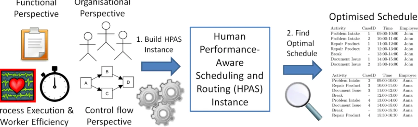
One of the goals of our work is to show that business process knowledge can be used in the context of workforce scheduling. We have formulated the HPAS scheduling problem in Section 2, and specified the necessary inputs to construct such a problem instance. In this section we discuss which elements from the field of BPM can be used in this setting, leading to an overall scheduling approach as shown in Figure 1.
Figure 1.An overview of the use of business process knowledge in scheduling. To create the HPAS problem instance as specified in Section 2 we need to determine various input parameters that can be linked to specific aspects from the field of process management.
last input, process execution measurements and information on the performance of people relates to the efficiency levels of workers and the processing times of jobs.
Some of this information needed to construct a HPAS instance is easily obtained and specified, e.g. the jobs that need to be scheduled and their allowed processing locations, while other inputs need to be derived or calculated, e.g. the relations between worker efficiency and estimated processing times. In the remainder of this section we discuss how to obtain the non-trivial problem inputs.
4.1 Organisational Perspective
The organisational perspective of a process provides several of the parameters for the scheduling of a workforce. It is generally straightforward to obtain an overview of the locations involved in a process and to specify where each activity can be performed. Most activities either have a fixed location, e.g. jobs involving physical presence at a specific customer or patient [33], or no location restrictions, e.g. electronic work that can be accessed using IT solutions [5], [34]. In many situations it is also clear which workers or organisational roles can be involved in each activity. However, this information may need to be transformed to the format of skills and skill requirements introduced in Section 2.
A process description may specify that an activity can be performed by members of a specific organisational unit, a role, specific employees or workers with a specific skill set [7]. In our HPAS problem description we only accounted for the requirement of specific skills for the execution of jobs, but the other situations can be easily modelled using artificial skills. For instance, if a job in a purchasing process requires an employee from the financial department then an artificial skill financial department can be created, assigned to all workers from the financial department and added as a requirement to any job requiring an employee from this organisational unit. In this way it is possible to create an arbitrary mapping specifying the organisational requirements for jobs in the form of skills.
4.2 Determining Worker Efficiency
The integration of dynamic human performance is one of the core elements of the HPAS problem. However, it is not easy to determine the input parameters for this aspect of the scheduling problem [15]. This has to do with the complex nature of human performance, which we discussed in Section 2.2.
activity is assumed to have a minimal and a maximal duration, i.e. the time it is expected to take for the job to be completed when the workers are at optimal or worst efficiency, respectively. These durations can be established using performance measurements under the assumption that the jobs that need to be scheduled can be compared to previous jobs for which performance measurements are available. In this way worker experience and individual performance differences are taken into account.
Additionally, the problem statement specifies that the workload of a worker causes job-specific exhaustion that may reduce the efficiency of workers. Depending on the available data, different models can be chosen to predict dynamic human performance based on workload. For instance, [15] provides a model to determine the distributions of performance variables based on the effects of taskload, where a higher taskload results in lower performance. Taskload in this case is simply the percentage of time during which the worker was performing a given set of tasks during a specific time period. This is comparable to the way that performing jobs decreases the efficiency level of workers and idle times relax and improve the efficiency level of workers in our problem statement.
As the work of [14] has shown, there are also links between stress, workload and performance. [13] provides a method to predict the performance of workers using data from wearable biosensors that measure galvanic skin response, a popular measurable indicator of stress. Establishing such models can explain how the efficiency of workers is affected by specific jobs that cause stress or exhaustion. These models can then be used to calculate individual and context-dependent performance estimates to be used in the scheduling problem.
4.3 Functional and Control Flow Perspectives
The functional perspective is the most basic process perspective, representing the process elements being performed and therefore being closely related to the jobs in a scheduling context. However, the most well-known process perspective is the control flow perspective, which expresses the behaviour allowed by the process in terms of its executions. Process models usually combine both perspectives and describe the allowed ordering of activities [6], [7], which means that they contain information on the jobs to be scheduled and their precedence relations. In this section we provide an approach to incorporate process models in the form of process trees [35], [36], a formalism to specify block-structured workflow nets [4], into our scheduling problem.
There exist many different process model notations [4], [7], but most traditional modelling languages allow the creation of models that are notsound, i.e. these models may contain deadlocks, livelocks and other anomalies. Process trees, however, are guaranteed to represent sound process models and their structure enables a more straightforward mapping between process knowledge and scheduling input.
Figure 2 shows the possible operators that process trees can be composed of, and their translations to BPMN constructs [35], [36]. Operator nodes specify the relation between their children. The five available operator types are: sequential execution (→), parallel execution (∧), exclusive choice (×), non-exclusive choice (∨) and repeated execution ( ). Children of an operator node can again be operator nodes or they can be leaf nodes that represent the execution of an activity. The order of the children matters for the sequence and loop operators. The order of the children of a sequence operator specifies the order in which the children are executed (from left to right). Nodes can have an arbitrary number of children, except for loop nodes ( ) that always have three children. The left child is the ‘do’ part of the loop and after its execution either the middle child, the ‘redo’ part, may be executed or the right child, the ‘exit’ part, may be executed. After the execution of the ‘redo’ part the ‘do’ part is again enabled and the ‘exit’ part is disabled. Process trees can also contain unobservable activities, indicated with aτ.
Figure 2.The process tree operators and their relation to BPMN constructs
Figure 3.A process model for a simple hardware maintenance process
behaviour of the→operator matches that of thesequenceprocedure, while the∧operator matches thesetprocedure, and the×operator matches thechoiceprocedure. For the non-exclusive choice (∨) and repeated execution ( ) there is no direct translation between process tree operator and scheduling concept. The reason for this is that in a setting where the makespan of a schedule is minimized, it is not desirable to execute unnecessary activities. Hence a non-exclusive choice becomes an exclusive choice in a scheduling context and the loop becomes a sequence of a single ‘do’ and ‘exit’.
Figure 3 shows an example process model for a simple hardware maintenance process in the form of a process tree [35], [36] and a BPMN model [4]. Each instance of this process starts with the execution of a single Problem Intake (PI)activity. This is followed by the parallel execution of Arrange Service Evaluation (ASE) and a choice between aRepair Product (RR) or aReplace Product (RC). The Repair Product activity is followed by Test Product (TP), and in either case there is the option to perform a Redo Maintenance (RM) afterwards in order to execute a new round of activities. Finally, the process instance ends whenDocument Incident (DI)is executed.
choice ×with sub-procedures {→2, RC}. This collection of scheduling procedures represents a single execution or process instance of this process model.
Note that the -operator has been assumed to be executed once without redo. However, a process model can express complex constructs such as choices or repetition, which need special considerations when deducing the scheduling procedures from a process model. We discuss this in the next subsection in more detail.
In the above example we constructed the procedures belonging to a single execution of a process. However, in general there are often many process instances being executed concurrently, possibly described by different process models. To create a scheduling problem instance where activities from different process instances are competing for the same resources, the deduction of the procedures is simply repeated for each process instance to be scheduled.
4.4 Choices and Repetition
In practice, the choices made and repetitions executed often depend on factors that are difficult to consider during the creation of a schedule. For instance, some choices may depend on external events or data, so called non-controllable choices, while controllable choices can be decided by the people executing the process [37]. Historical information may be used in order to estimate the expected activity executions and non-controllable choices made. During the creation of the scheduling problem, this information can then be used to omit the branches of non-controllable choices that are not expected to be executed for a given process instance. However, we retain controllable choices in our scheduling problem, which are not fixed by the characteristics of a given process instance or external input, in order to allow the scheduling approach to make the best choice for a better process execution. Dealing with repetition is similar to handling non-controllable choices, as we assume that repeating activities are not desirable in our scheduling context.
For each process instance, we need to determine what the controllable and uncontrollable choices and repetition are, which requires domain knowledge of the process. In the process model shown in Figure 3 there is a choice and a cycle: a choice between a repair and a replacement and an option to restart the maintenance cycle. The choice between repairing or replacing the product is controllable, so this results in a choice procedure in the HPAS instance with two alternative sub-procedures. The option to restart the maintenance depends on the success of the previous activities, so this repetition is in any case uncontrollable and therefore deciding whether or not to restart the maintenance cycle cannot be part of the scheduling problem.
Handling an uncontrollable choice or repetition depends on previous process performance measurements. If the maintenance cycle is only repeated rarely then this activity can be omitted from the list of jobs to be scheduled. Alternatively, an estimation can be made for the number of process instances that will feature a repeated maintenance. For these process instances we need to take care of the repetition in the model to arrive at a finite set of jobs and procedures representing their execution.
5
Solving HPAS Instances
As shown in Figure 1, once we have created a HPAS instance as described in Section 4 we need to solve it to obtain optimised schedules. We have formulated our scheduling problem as a Mixed Integer Linear Programming (MILP) model, which is included below. This MILP model has been implemented and can be solved with CPLEX [38].
The formulation of the MILP model is relatively straightforward from the problem statement defined in Section 2. The notation from Section 2.3 is summarized in Table 1. The exact relations between worker efficiency levels and job durations are not explicitly specified in the problem statement. The reason for this is that these relations are heavily affected by a trade-off between model complexity and realism. As stated in Section 4.2, there are complex models that can be used to predict dynamic human performance based on historical performance measurements. Instead of these complex models we chose to assume a job-specific linear dependency between efficiency and job durations for ease of understanding and computational efficiency.
We also simplified the modelling of choice procedures slightly by restricting that a choice
procedure cannot contain anotherchoiceas a sub-procedure. The reason for this was to reduce the complexity of the MILP model, as the size of the scheduling problems that can be solved using this implementation is limited.
The MILP model has several constraints that use Big M coefficients to formulate our nonlinear scheduling problem in a way that can be solved using linear programming. The coefficients are used to trivially enable certain constraints using indicator variables, e.g. to only specify activity durations for the jobs that are actually executed.
Table 1 gives the notation used in our MILP model, i.e. sets, indices, parameters, and decision variables.
Minimize Cmax (10)
subject to
sj+λj ≤Cmax, j ∈ J (11)
X
pq∈p
execpq = 1, p∈ Pxor (12)
xj =execpq, j ∈jobs(pq), pq∈p, p ∈ Pxor (13)
X
n∈Nj
yj,n =xj, j ∈ J (14)
sj0 +λj0−M(1−xj0)≤sj, j ∈ J, j0 ∈P REDj (15)
Rj−M(1−xj)≤sj ≤Dj −λj, j ∈ J (16)
X
w∈W
SKws
Imax X
i=1
zw,i,j ≥SRsjxj, j ∈ J, s∈ S (17)
X
j∈J
Table 1.Sets, parameters, and decision variables
Sets
S set of skill domains,s∈ S N set of all locations,n∈ N W set of all workers,w∈ W
J set of all jobs,j∈ J,J =JM an∪ JOpt Pxor set of all choice procedures,p∈ Pxor
Parameters
Tn,n0 travel time to go from locationnton0 Nj allowed processing locations of jobj
SKw skills of workerw,SKw∈ {0,1}S×L
SRj skill requirements of jobj,SRj ∈NS×L Rj, Dj release and due date of jobj
P REDj predecessors of jobj,P REDj ⊆ J \ {j}
Pj minimum processing time of jobj
ρj rate at which the duration of jobjis increased due to worker inefficiency
δj exhaustion ratio by which efficiency decreases after performing jobj,δj ∈(0,1)
EC+ efficiency level change due to relaxing or travelling in unit time
Imax maximum size of any job sequences of workers
jobs(pq)set of jobs in sub-procedurepq∈p, of choicep∈ Pxor,jobs(pq)⊂ JOpt
Decision Variables
Cmax makespan of the schedule
sj, λj start time, and duration of jobj
execa indicates if alternativeais executed,a∈c,c∈ C
xj indicates if jobjis executed
yj,n indicates if processing locationlocj of jobjisn, wheren∈ Nj
zw,i,j indicates if jobjisithjob in the job sequence of workerw, i.e.jsw(i) =j
deptw,i departure time of workerwat the processing location ofjsw(i)
τw,i travel time of workerwfrom processing location ofjsw(i−1)to the one ofjsw(i)
elw,i efficiency level of workerwwhen starting to process jobjsw(i)
el−w,i efficiency level change of workerwdue to processing jobjsw(i)
Imax X
i=1
zw,i,j ≤xj, w∈ W, j ∈ J (19)
X
j∈J
zw,i,j ≤
X
j∈J
zw,i−1,j, w∈ W, i≤Imax (20)
deptw,i−1+τw,i−M(1−zw,i,j)≤sj, j ∈ J, w ∈ W, i≤Imax (21)
sj+λj −M(1−zw,i,j)≤deptw,i, j ∈ J, w ∈ W, i≤Imax (22)
Tn,n0 −M(4−yj,n−yj0,n0 −zw,i−1,j−zw,i,j0)≤τw,i,
j, j0 ∈ J, n ∈ Nj, n0 ∈ Nj0, w ∈ W, i≤Imax (23)
elw,i−1−elw,i−− 1+EC +
(sj−deptw,i−1)−M(1−zw,i,j)≥elw,i,
j ∈ J, w ∈ W, i≤Imax (25)
Pj ∗(1 +ρj(1−elw,i))−M(1−zw,i,j)≤λj, j ∈ J, w ∈ W, i≤Imax (26)
execpq ∈ {0,1}, pq ∈p, p∈ Pxor (27)
yj,n ∈ {0,1}, j ∈ J ∪ JOpt, n ∈ Nj (28)
zw,i,j ∈ {0,1}, j ∈ J ∪ JOpt, w ∈ W,1≤i≤Imax (29)
Then the MILP model is given by constraints (10)–(29). The first constraint (10) is the objective function which is minimized. Constraint (11) is used to find the makespan of the schedule. Constraints (12)–(13) ensure that only one alternative sub-procedure is executed per choice. Mandatory jobs are always executed, i.e. xj = 1for all j ∈ JM an, so we definexj variables for
jobs inJM anonly for the simplicity of the MILP formulation. Every job should be executed exactly
in one location (constraints (14)), and precedence relations should be satisfied (constraints(15)). Executions of jobs should be between their release and due dates (constraints(16)), and they should be executed by a group of workers who have requested skills to do so (constraints(17)). Assignment between workers and jobs are expressed by constraints (18)–(20). Constraints (21)–(23) ensure that each worker has a route while executing the jobs and temporal constraints are satisfied, i.e. departures, start times, and travel times. Constraints (24)–(26) are used to obtain correct efficiency level of workers after job executions and efficiency-dependent job durations. Note that the efficiency level update in constraints (25) considers efficiency changes of a worker due to job execution as well as efficiency changes due to non-working times like breaks and travels. Finally, constraints (27)–(29) enforce that choice-sub-procedure-execution, job-location and worker-job assignment variables should be binary.
6
Evaluation
In this section we present an evaluation of the MILP implementation introduced above. The main goals of the evaluation are to show that dynamic human performance can be taken into account in scheduling and to understand how the inclusion of dynamic performance differences in scheduling affects the complexity of the problem. Therefore, we created a simulation model and compared the simulated performance to the schedules generated by our approach. We also tested the ability of the MILP implementation to solve different scheduling problems of varying difficulty within a set time limit. The evaluation was performed using CPLEX V12.6.0 [38] on a PC with a 3.4 GHz quad-core processor and 16 GB RAM memory.
6.1 Example Process Simulation
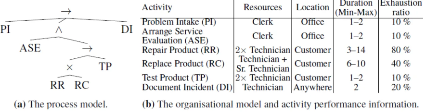
We created a simulation model of a simple hardware maintenance process using CPN Tools [39]. The process knowledge used in this simulation is shown in Figure 4. This information was also used in the creation of a HPAS problem instance, as discussed in Section 4.
Figure 4.The process knowledge for a simple hardware maintenance process, as used in our simulation
is assumed that the role of Senior Technician may also perform any job requiring a Technician. Different process instances may involve different customers and hence different locations.
Both CPN Tools and our MILP scheduling implementation use discrete time. The minimum and maximum job durations mentioned in Figure 4b are given in discrete time units, with the realised job durations depending on worker efficiency linearly. The travel distance between the
Officelocation and the variousCustomerswas set to 1 time unit.
Both the simulation and the HPAS instance were used to obtain schedules for the above process description. Figure 5 and Figure 6 show the optimal schedule as provided by the CPLEX solver and an example obtained from the simulation model. Comparing the simulated schedule and the optimal one shows that under this human performance model it is more efficient to balance workload and rest. This is also highlighted by the average utility of workers, which is68 %in the optimal solution and90 %in the simulation model if jobs are executed as soon as possible.
Figure 5.The optimal scheduling of 3 process instances of the process described in Figure 4
Figure 6. An example schedule for 3 process instances generated by the simulation model of the process described in Figure 4
6.2 Parameter Effects on Complexity
flow. We evaluated the solutions with and without taking into account each of the four aspects, for a total of 16 different possible combinations.
The instances were generated randomly with a fixed number of jobs and workers, and other parameters falling into a range depending on the selected aspect combinations. Each instance included 20 jobs and 10 workers, which was based on memory and process time requirements during initial testing and comparable to e.g. the instance sizes used in the evaluation of [33], [40].
For the routing aspect there was a setting with some basic movement of workers between four different locations arranged sequentially. The network of locations was kept very simple because initial tests showed that complex routing requirements would already result in very difficult problems, even without taking into account the scheduling of the activities. Each job was randomly assigned to one out of four locations. When routing was not taken into account each job was assigned to the same location and workers had no need to travel.
For the skill requirement aspect we introduced 10 skill domains, similar to the instances from [40]. The workers and jobs were divided randomly into three different groups of roughly equal size: one requiring or possessing a single random skill, one requiring or possessing every skill and one requiring or possessing half of the skills. When skill requirements were not taken into consideration, there was only a single skill that every worker possessed and every job required.
The efficiency aspect introduced job-specific durations and effects on efficiency. Each job had a 50 % chance to have a duration affected by worker efficiency. Each job also had an independent 50 % chance to have an effect on worker efficiency. When worker efficiency was not taken into account each job had a fixed duration and no effect on worker efficiency.
The control flow aspect concerned the presence of job predecessors and choices between jobs. In this setting there was a random set of generated procedures resulting in 10 precedence constraints and 2 choices between alternative jobs. When the control flow aspect was not taken into account there were no choices or predecessors amongst the scheduled jobs.
6.3 Complexity Results
For each of the 16 parameter aspect combinations introduced above we generated 20 random instances for a total of 320 scheduling problem instances. The MILP implementation was given up to 5 minutes to solve each scheduling instance. The results are shown in Table 2.
Table 2. The results of the evaluation, with time measured in seconds and also showing the percentage of instances for which a feasible or optimal solution could be found within the time limit. Each scenario consisted of 160 instances, i.e. 20 instances for each of the 8 combinations of the 3 other aspects.
Scenario Average Time to Feasible after Average Time to Optimal after Feasible (Stdev.) 300 seconds Optimal (Stdev.) 300 seconds
No routing 6.0 (24.2) 93 % 35.9 (52.4) 31 %
Routing 4.9 (15.7) 89 % 63.2 (67.7) 32 %
No skill requirements 2.5 (4.0) 100 % 35.0 (43.5) 49 % Skill requirements 9.1 (29.8) 83 % 104.1 (86.7) 13 % No worker efficiency 2.7 (7.4) 85 % 17.0 (27.5) 33 % Worker efficiency 7.8 (27.0) 98 % 85.3 (68.9) 30 %
No control flow 1.2 (1.1) 100 % - (-) 0 %
Control flow 10.6 (29.7) 83 % 49.8 (61.8) 63 %
was taken into account, so including this aspect in the scheduling problem does not appear to make it more difficult to obtain a feasible solution.
The results are quite different when considering the time and likelihood required to obtain an optimal solution. For the inclusion of the routing, skill requirements and worker efficiency aspects the average time required to obtain an optimal solution increased significantly. However, both routing and worker efficiency appear to have little effect on the likelihood to obtain an optimal solution. The inclusion of skill requirements did have a significant negative effect on both the time and the likelihood required to obtain an optimal solution. Interestingly, in the absence of control flow constraints the current implementation was not able to find any optimal solutions. Finding an optimal solution appears to be highly dependent on the parameter settings, but the inclusion of worker efficiency is not a major factor in the solver’s ability to obtain an optimal solution.
To explore why the implementation was unable to find the optimal scheduling solution in the absence of control flow constraints, we performed a manual study of several easy problem instances. It was found that the solver was able to find a solution that was actually optimal, but it was not able to confirm the solution’s optimality within the time limit. This is most likely related to the fact that in these instances the solver appears to explore and enumerate all possible orderings of jobs within the other restrictions such as worker assignment. Upon reducing the size of the generated problem instances to 10 jobs and 5 workers the solver was able to prove the optimality of the discovered solutions within seconds. Repeated testing with increasing problem instance sizes revealed that there appeared to be a cut-off point where the solver was no longer able to determine optimality using branch-and-bound methods. At that point it reverted to enumerating all possible job assignment combinations.
The above evaluation shows that the scheduling of activities affected by dynamic human performance is a difficult problem. Even for a small simulated environment, the current model often cannot be solved to obtain an optimal schedule, although finding feasible solutions is generally possible. Additional research is required to show the application of dynamic human performance in a real-life setting to demonstrate its value.
7
Conclusions
In this article we have shown how dynamic human performance may influence the scheduling process. To the best of our knowledge, this is the first attempt to incorporate worker efficiency as a concept into workforce scheduling and routing. For the sake of clarity, we assumed that (1) job durations are affected proportionally by the worst performance level of assigned workers, and (2) worker performances decrease when performing jobs proportional to their current levels. Accordingly, we provided a formal description of the HPAS scheduling problem, and specified feasibility conditions in Section 2. Then we discussed how various aspects from the field of Business Process Management relate to the parameters of this scheduling problem and how they can be established. We also formulated the HPAS scheduling problem as a MILP model. Finally, we showed that scheduling instances of limited size can be solved by using our MILP model. Regarding our experimentation, we may conclude that taking into account dynamic worker efficiency does not significantly increase the hardness of solving scheduling instances that we have generated compared to traditional extensions of the scheduling problem such as skill levels and routing.
Another research direction is the development of a Large Neighborhood Search method for our scheduling problem. In an LNS method, destroying and repairing heuristics should be carefully designed such that the worker efficiency levels are maintained correctly after every improvement iteration.
The main limitation of this work is that the evaluation was performed on a simulation model of a business process. The way how worker efficiencies affect the realisation of schedules highly depends on the type of industry sector and the processes and people involved. To increase the realism of the efficiency model it is necessary to do case studies to apply our scheduling approach in practice and study the results. With the advent of wearable sensor technologies, the first steps have been taken to measure stress and workload in order to obtain the individual models of performance that enable this.
References
[1] S. Hartmann and D. Briskorn, “A survey of variants and extensions of the resource-constrained project scheduling problem,” European Journal of Operational Research, vol. 207, no. 1, pp. 1–14, 2010. [Online]. Available: https://doi.org/10.1016/j.ejor.2009.11.005
[2] P. Brucker, A. Drexl, R. M¨ohring, K. Neumann, and E. Pesch, “Resource-constrained project scheduling: Notation, classification, models, and methods,”European Journal of Operational
Research, vol. 112, no. 1, pp. 3–41, 1999. [Online]. Available: https://doi.org/10.1016/S0377-2217(98)
00204-5
[3] J. V. den Bergh, J. Beli¨en, P. D. Bruecker, E. Demeulemeester, and L. D. Boeck, “Personnel scheduling: A literature review,” European Journal of Operational Research, vol. 226, no. 3, pp. 367–385, 2013. [Online]. Available: http://dx.doi.org/10.1016/j.ejor.2012.11.029
[4] W. M. P. van der Aalst, Process Mining: Discovery, Conformance and Enhancement of Business
Processes. Springer, 2011.
[5] A. Goel, V. Gruhn, and T. Richter, “Mobile workforce scheduling problem with multitask-processes,”
inInternational Conference on Business Process Management. Springer, 2009, pp. 81–91. [Online].
Available: https://doi.org/10.1007/978-3-642-12186-9 9
[6] B. Curtis, M. I. Kellner, and J. Over, “Process modeling,”Communications of the ACM, vol. 35, no. 9, pp. 75–90, 1992. [Online]. Available: https://doi.org/10.1145/130994.130998
[7] B. List and B. Korherr, “An evaluation of conceptual business process modelling languages,” in
Proceedings of the 2006 ACM symposium on Applied computing. ACM, 2006, pp. 1532–1539.
[Online]. Available: https://doi.org/10.1145/1141277.1141633
[8] J. C. Goodale and E. Tunc, “Tour scheduling with dynamic service rates,” International
Journal of Service Industry Management, vol. 9, no. 3, pp. 226–247, 1998. [Online]. Available:
https://doi.org/10.1108/09564239810223538
[9] M. A. Staal, “Stress, cognition, and human performance: A literature review and conceptual framework,”Hanover, MD: National Aeronautics and Space Administration, 2004.
[10] M. Westman and D. Eden, “The inverted-u relationship between stress and performance: A field study,” Work & Stress, vol. 10, no. 2, pp. 165–173, 1996. [Online]. Available: https://doi.org/10.1080/02678379608256795
[11] M. Jamal, “Job stress and job performance controversy: An empirical assessment,” Organizational
behavior and human performance, vol. 33, no. 1, pp. 1–21, 1984. [Online]. Available:
[12] R. Kocielnik, N. Sidorova, F. M. Maggi, M. Ouwerkerk, and J. H. D. M. Westerink, “Smart technologies for long-term stress monitoring at work,” inProceedings of the 26th IEEE International
Symposium on Computer-Based Medical Systems, Porto, Portugal, June 20-22, 2013, 2013, pp.
53–58. [Online]. Available: https://doi.org/10.1109/cbms.2013.6627764
[13] C. Mundell, J. P. Vielma, and T. Zaman, “Predicting performance under stressful conditions using galvanic skin response,”CoRR, vol. abs/1606.01836, 2016.
[14] M. Bernburg, K. Vitzthum, D. A. Groneberg, and S. Mache, “Physicians’ occupational stress, depressive symptoms and work ability in relation to their working environment: a cross-sectional study of differences among medical residents with various specialties working in german hospitals,” BMJ open, vol. 6, no. 6, p. e011369, 2016. [Online]. Available: https://doi.org/10.1136/bmjopen-2016-011369
[15] E. M. Rantanen and B. R. Levinthal, “Time-based modeling of human performance,” inProceedings
of the Human Factors and Ergonomics Society Annual Meeting, vol. 49, no. 12. SAGE Publications,
2005, pp. 1200–1204.
[16] R. M. Yerkes and J. D. Dodson, “The relation of strength of stimulus to rapidity of habit-formation,”
Journal of comparative neurology and psychology, vol. 18, no. 5, pp. 459–482, 1908. [Online].
Available: https://doi.org/10.1002/cne.920180503
[17] A. A. Kovacs, S. N. Parragh, K. F. Doerner, and R. F. Hartl, “Adaptive large neighborhood search for service technician routing and scheduling problems,” Journal of Scheduling, vol. 15, no. 5, pp. 579–600, 2012. [Online]. Available: https://doi.org/10.1007/s10951-011-0246-9
[18] M. Fırat and C. Hurkens, “An improved mip-based approach for a multi-skill workforce scheduling problem,”Journal of Scheduling, vol. 15, no. 3, pp. 363–380, 2012. [Online]. Available: https://doi.org/10.1007/s10951-011-0245-x
[19] J.-F. Cordeau, G. Laporte, F. Pasin, and S. Ropke, “Scheduling technicians and tasks in a telecommunications company,” Journal of Scheduling, vol. 13, no. 4, pp. 393–409, 2010. [Online]. Available: https://doi.org/10.1007/s10951-010-0188-7
[20] B. Elbenani, J. A. Ferland, and V. Gascon, “Mathematical programming approach for routing home care nurses,” in 2008 IEEE International Conference on Industrial Engineering and Engineering
Management, Dec 2008, pp. 107–111. [Online]. Available: https://doi.org/10.1109/ieem.2008.
4737841
[21] S. V. Begur, D. M. Miller, and J. R. Weaver, “An Integrated Spatial DSS for Scheduling and Routing Home-Health-Care Nurses,”Interfaces, vol. 27, no. 4, pp. 35–48, 1997. [Online]. Available: https://doi.org/10.1287/inte.27.4.35
[22] P. Cappanera, L. Gouveia, and M. G. Scutell`a, The Skill Vehicle Routing Problem. Berlin, Heidelberg: Springer Berlin Heidelberg, 2011, pp. 354–364. [Online]. Available: http://dx.doi.org/10. 1007/978-3-642-21527-8 40
[23] A. Goel and F. Meisel, “Workforce routing and scheduling for electricity network maintenance with downtime minimization,”European Journal of Operational Research, vol. 231, no. 1, pp. 210 – 228, 2013. [Online]. Available: https://doi.org/10.1016/j.ejor.2013.05.021
[24] J. D´ıaz-Ram´ırez, J. I. Huertas, and F. Trigos, “Aircraft maintenance, routing, and crew scheduling planning for airlines with a single fleet and a single maintenance and crew base,”Computers Industrial
Engineering, vol. 75, pp. 68 – 78, 2014. [Online]. Available: https://doi.org/10.1016/j.cie.2014.05.027
[25] V. Pillac, C. Gu´eret, and A. Medaglia, “On the Technician Routing and Scheduling Problem,” in
Metaheuristics International Conference (MIC) 2011, Udine, Italy, Jul. 2011, pp. S2–40–1, iSBN
[26] P. Toth, D. Vigo, P. Toth, and D. Vigo,Vehicle Routing: Problems, Methods, and Applications, Second
Edition. Philadelphia, PA, USA: Society for Industrial and Applied Mathematics, 2014. [Online].
Available: https://doi.org/10.1137/1.9781611973594
[27] D. Bredstr¨om and M. R¨onnqvist, “Combined vehicle routing and scheduling with temporal precedence and synchronization constraints,” European Journal of Operational Research, vol. 191, no. 1, pp. 19–31, 2008. [Online]. Available: https://doi.org/10.1016/j.ejor.2007.07.033
[28] U. Belhe and A. Kusiak, “Resource constrained scheduling of hierarchically structured design activity networks,” IEEE Transactions on Engineering Management, vol. 42, no. 2, pp. 150–158, 1995. [Online]. Available: https://doi.org/10.1109/17.387271
[29] S. A. Slotnick, “Order acceptance and scheduling: A taxonomy and review,” European
Journal of Operational Research, vol. 212, no. 1, pp. 1–11, 2011. [Online]. Available:
https://doi.org/10.1016/j.ejor.2010.09.042
[30] D. Shabtay, N. Gaspar, and M. Kaspi, “A survey on offline scheduling with rejection,” Journal
of Scheduling, vol. 16, no. 1, pp. 3–28, 2013. [Online]. Available: https://doi.org/10.1007/
s10951-012-0303-z
[31] M. Ebben, E. Hans, and F. O. Weghuis, “Workload based order acceptance in job shop environments,” OR spectrum, vol. 27, no. 1, pp. 107–122, January 2005. [Online]. Available: https://doi.org/10.1007/s00291-004-0171-9
[32] F. T. Nobibon and R. Leus, “Exact algorithms for a generalization of the order acceptance and scheduling problem in a single-machine environment,” Computers & Operations Research, vol. 38, no. 1, pp. 367–378, 2011. [Online]. Available: https://doi.org/10.1016/j.cor.2010.06.003
[33] R. B. Bachouch, A. Guinet, and S. Hajri-Gabouj, “An optimization model for task assignment in home health care,” in Health Care Management (WHCM), 2010 IEEE Workshop on. IEEE, 2010, pp. 1–6. [Online]. Available: https://doi.org/10.1109/whcm.2010.5441277
[34] E. E. Kossek and J. Michel, “Flexible work schedules,” Handbook of industrial-organizational
psychology, vol. 1, pp. 535–72, 2010.
[35] J. C. A. M. Buijs, “Flexible evolutionary algorithms for mining structured process models,” Ph.D. dissertation, Ph.D. thesis, Technische Universiteit Eindhoven, 2014. [Online]. Available: https://pure.tue.nl/ws/files/4032592/780920.pdf
[36] M. L. van Eck, J. C. A. M. Buijs, and B. F. van Dongen, “Genetic process mining: Alignment-based process model mutation,” in Business Process Management Workshops - BPM 2014 International
Workshops, Eindhoven, The Netherlands, September 7-8, 2014, Revised Papers, 2014, pp. 291–303.
[Online]. Available: https://doi.org/10.1007/978-3-319-15895-2 25
[37] J. Dehnert, “Non-controllable choice robustness expressing the controllability of workflow processes,”
inInternational Conference on Application and Theory of Petri Nets. Springer, 2002, pp. 121–141.
[Online]. Available: https://doi.org/10.1007/3-540-48068-4 9
[38] I. ILOG, “Ibm ilog cplex optimization studio,” 2015. [Online]. Available: https://www.ibm.com/ software/products/en/ibmilogcpleoptistud
[39] K. Jensen, L. M. Kristensen, and L. Wells, “Coloured Petri Nets and CPN Tools for modelling and validation of concurrent systems,”International Journal on Software Tools for Technology Transfer, vol. 9, no. 3-4, pp. 213–254, 2007. [Online]. Available: https://doi.org/10.1007/s10009-007-0038-x