The use of weights to account for non-response and drop-out

The use of weights to account for non-response and drop-out

Max-Planck-Institut of Psychiatry, Clinical Psychology and Epidemiology Kraepelinstr. 2–10 80804 München, Germany E-Mail: [email protected]

H.-U. Wittchen, PhD Technical University Dresden Institute of Clinical Psychology & Psychotherapy Dresden, Germany Soc Psychiatry

Abstract

Background Empirical studies in psychiatric research and other fields often show substantially high refusal and drop-out rates. Non-participation and drop-out may introduce a bias whose magnitude depends on how strongly its determinants are related to the respective parameter of interest. Methods When most information is missing, the standard approach is to estimate each respondent’s probability of participating and assign each respondent a weight that is inversely proportional to this probability. This paper contains a review of the major ideas and principles regarding the computation of statistical weights and the analysis of weighted data.

Results A short software review for weighted data is provided and the use of statistical weights is illustrated through data from the EDSP (Early Developmental Stages of Psychopathology) Study. The results show that disregarding different sampling and response probabilities can have a major impact on estimated odds ratios.

Conclusions The benefit of using statistical weights in reducing sampling bias should be balanced against increased variances in the weighted parameter estimates.

Key words: selection bias, non-response, drop-out, missing values, weighting, survey

Sampling bias due to systematic non-response or drop-out

Non-participation is a common problem in various scientific fields like social sciences, economy and the epidemiology of mental disorders. Unlike missing values of specific variables, whole units of observation are missing. Researchers usually assume that refusal is almost never a pure random process, that is, a process that is independent of all the

phenomena under consideration. Instead, participation is assumed to be influenced by these phenomena (Greenland 1977; Levy and Lemeshow 1999, p. 393ff.). Kessler et al. (1995) cited some papers that had demonstrated elevated refusal rates in the presence of a history of mental disorders and treatment. For instance, Allehoff et al. (1983) found that, in a general population study on mental disorders among 8-year-old children, non-participation or drop-out (rate=38.5%) was associated with lower IQ values and scholastic difficulties. The problem of non-response has apparently increased during the until 1995 decades (Kessler et al. 1995). In longitudinal studies, the magnitude of this problem increases further when participation during the whole course of a study is required. For example, in a cohort study from the US, Preisser et al. (2000) have found that cigarette smokers were more likely to drop out of the study. Consider the case where 70% of the sampled units complete the first investigation and, in each of two consecutive waves of assessments, another 15% of the remaining participants drop out of the study. This would result in a completion rate for the entire study of only 50.6%. Even in cross-sectional studies in psychiatric epidemiology, completion rates typically do not exceed 80% and are often even much lower. Clearly, selection bias can not only arise from systematic non-response and drop-out but also from different sampling probabilities induced by the study design. In practice, one may apply the heuristics that the poorer a

response rate is, the more likely is a substantial bias due to non-participation. A non-response rate of, say, 10% will probably not induce a strong bias unless non-participation is strongly associated with the parameters of interest. The optimal strategy to overcome non-participation is to maximize the response rate during the data collection process as “you can’t fix by

analysis what you bungled by design” (Light et al.1990). For an overview on strategies to improve completion rates, see Kessler et al. (1995) and Levy and Lemeshow (1999, p. 395ff). Usually,more resources are required to increase a participation rate from, say, 70% to 80 % than from 60 % to 70% because, at the end of the study phase, those individuals who are difficult to contact and unwilling to participate tend to cumulate. Thus, there is typically no linear association between the participation rate and the costs of a survey, and restrictions in financial and personal resources often result in insufficient completion rates. In this paper, we give an outline on the computation of statistical weights to adjust for sampling bias and the analysis of weighted data. A short review on software for weighted data is provided and the use of statistical weights is exemplified through data from the EDSP Study (Wittchen et al. 1998a, b; Lieb et al. 2000).

Weighting and other methods to compensate for non-participation

The easiest statistical strategy to deal with unit response or drop-out is to omit the non-respondents or drop-out cases and analyse the data under the assumption that every unit entered the sample with equal probability. Clearly, any difference between responders and non-responders that is related to the parameter of interest will introduce sampling bias. Through decreased participation rates in the past, the attention has been drawn to statistical methods meant to reduce the selection bias introduced by non-response or drop-out. If the distributions of certain characteristics such as sex or age in the target population are known from external data sources and these variables are collected in the study, non-response related to those characteristics can be assessed and adjusted for by weighting the responders (see below). This method is called post-stratification (Kessler et al. 1995). In Germany and other

European countries, for instance, the exact distributions of age, gender and geographical location in the target population are known through the registry databases. A different approach not covered in this paper referred to as doublesampling collects at least some basic

socio-demographic information among a randomly selected subsample of the non-participants (and of all participants) (Levy and Lemeshow 1999,p. 402 ff.). In longitudinal studies,

information on the characteristics of drop-out cases is available from prior assessment waves. There are three major statistical approaches to address non-response or drop-out: (1) the imputation of missing values, (2) the consideration of non-participation or drop-out within statistical models, and (3) the assignment of statistical weights to the participants. In this paper, we focus on the latter method as it is the most appropriate approach for the scenario mainly covered in this paper, where entire data sets are missing except for some basic socio-demographic information. A detailed description of the other methods is beyond the scope of this article. Briefly, especially the multiple imputation method for missing values has received increasing attraction in recent years. The observed data are used to estimate the missing values, and multiple completed data sets are created by drawing different random numbers from the posterior predictive distribution of the missing value (e. g. Rubin and Schenker

1991). Multiple imputation accounts for the variance introduced by drawing random numbers; a single imputation would treat the imputed values as true observations and, thus, under-estimate the variance in the target parameter. This method has the advantage that, after imputation, every kind of statistical analysis is possible, which makes it particularly suitable for public use. Furthermore, globally applicable formulas exist for pooled point estimates and confidence intervals across the different imputed data sets (repeated-imputation inference) (e. g. Rubin and Schenker 1991; Rubin 1996). Besides, unlike the weighting method, this

approach requires no omission of cases provided that at least several values are observed. On the other hand, this method is not intended to be used for a fraction of more than 50 % missing information (Rubin 2003). For an overview of sophisticated data imputation

procedures within particular statistical models via the EM algorithm, consult, for instance, the textbook by Schafer (1997). Diggle et al. (1994) have provided an outline of statistical models that incorporate the drop-out process in longitudinal studies. Here, sensitivity analyses that analyse the impact of some potential scenarios of non-response on the results are of particular interest (e. g. Scharfstein et al. 1999; Touloumi et al. 2002). For a review on statistical models (Bayesian models, sensitivity analyses and simulation techniques) to address multiple bias arising not only from non-participation, see Greenland (in press).

Sampling designs

The weights in statistical analyses are designed to compensate differences in participation rates introduced by different sampling probabilities or unintended systematic non-response. Different sampling probabilities as well as non-response can occur at several selection stages. First, the subjects might have been sampled with different probabilities in different strata. In the EDSP Study, for instance, the younger individuals were oversampled because they were of particular interest and, hence, more statistical precision was required for them (see below). Another example refers to screening designs. In the epidemiology of mental disorders, a two-stage sampling design is sometimes used. Usually, the subjects are drawn with equal

probabilities at the first sampling stage, and each individual completes a screening instrument on mental problems. For the second stage, those who endorsed items on mental problems are sampled with a higher probability than those who did not. Consecutively, those who were sampled for the second stage complete a more costly and accurate instrument such as a structured diagnostic interview (e. g. Wittchen et al. 1999; Jacobi et al. 2002). The rationale behind this study design is the increasing efficiency of a sample: those who endorsed

symptoms on the screener are more likely to have mental disorders, and the expected number of cases with rare conditions increases. Finally, the participants using the costly instrument are assigned a weight based on the inverse probability of being sampled for the second stage. More detailed discussion of sample designs can be found in Levy and Lemeshow (1999) and Smith (2001).

The computation of statistical weights

Recently, the use of statistical weights has become increasingly prominent in statistics to adjust the distribution of the remaining subjects‘ characteristics to that of the target population (e. g. Rotnitzky and Robins 1997; Preisser et al. 2000;Yung and Rao 2000; Miller et al. 2001; Smith 2001). In this connection, it is important to note that the lack of sampling bias in the estimation of two marginal distributions (e. g. prevalence rates) does not imply a lack of bias in the estimation of the association between the corresponding variables (Greenland 1977). To demonstrate the key idea, we assume for the moment that sampling takes place only at one stage and depends only on a single variable. Usually, this variable is categorical. Imagine, for instance, that different age groups were sampled with different probabilities. Then the

sampling bias is removed by weighting the subjects with a weight proportional to the inverse sampling probability. To calculate the weighting variable, the inverse sampling probability of each individual in the sample is divided by the mean of the inverse sampling probabilities of all individuals. This yields a weighting variable that is scaled such that the mean weight of all individuals is 1 and the weighted sample size equals the actual, unweighted sample size. When more than one categorical variable is involved, cells for adjustment can be formed. Each cell contains a combination of the determinants of participation, and adjustment requires

that their joint distribution in the target population is known. This strategy, however, is only applicable to a – relative to the sample size – small number of determinants. Otherwise, the weight would be based on many low cell frequencies in the sample, and the resulting high variance in the weighting variable would yield a strong increase in confidence interval width (see below). Smoother weights can be obtained with models using the response indicator as outcome when some information is available also about the non-responders. The number of determinants can be reduced to a single variable, a so-called balancing score. Its aim is to estimate a certain individual’s propensity score which is, in this context, the estimated

probability that the individual completes the study on the basis of the information available for responders and non-responders (e. g. Heyting et al. 1992). The concept of propensity scores was originally developed to adjust for assignment bias in causal inference in non-randomized treatment and observational studies. The propensity score here is the probability of being assigned to one of two groups (Rosenbaum and Rubin 1983; Rosenbaum 2002). Balancing scores are often derived from logistic regression models (Kessler et al. 1995) because they tend to yield the smoothest fit to the data (McCullagh and Nelder 1989). A model should reduce the number of covariates to those with the highest predictive value in a suitable way, that is, the balancing score should have a low predictive standard deviation for each individual, and the model should fit the data. The omission of unnecessary covariates generally results in more stable predictions when the results are extrapolated to other

populations (McCullagh and Nelder 1989). The covariate selection and model specification to calculate a weight are always a trade-off between bias reduction and increase in variance of the weight. Bias reduction is assessed through the difference in point estimates between weighted and unweighted analysis, as well as between the use of different weights. Typically, the variance of the weighted estimator increases linearly with the variance of the weighting variable (Little et al. 1997). Hence, if added variance dominates bias reduction, the weighting variable should be modified to have a lower variance. Modifications to reduce variance include trimming (transformations that reduce the extreme tails of a distribution), shrinking (transformations where the distribution is shrunken toward the mean to reduce skewness), categorizing the weight (and assigning the average weight to the individuals within the same category) or collapsing given weight strata (Little et al. 1997, and references therein). As already mentioned, different sampling probabilities, non-response and drop-out can occur at different stages of sampling. To derive a statistical weight that compensates for different patterns of non-response at the different stages of selection, it is natural to multiply the statistical weights for the different stages because they reflect conditional probabilities of a participant’s entering the next stage given that the present stage has been completed (Kessler et al. 1995; Little et al. 1997). Statistically, this argument is based on the fact that every joint probability density function can be factorized into conditional densities over time (e. g. Cox and Wermuth 1996).

The analysis of weighted data

Once a statistical weight is established, it can, in principle, be applied to all analyses to be run with the data set. However, whether weighting is really necessary for a specific analysis and, if so, how much information is necessary to be considered in the weight depends on the specific parameter under consideration. Point estimates are usually modified by multiplying the contribution of each individual to a statistic by its statistical weight (e. g. to compute a weighted mean, each individual’s value of a variable is multiplied by the weight of that individual, then the sum over the individuals is calculated and divided by the sample size). The crucial issue in all analyses of weighted data is that the statistical weights do not represent true numbers of observations, but only expected numbers that would apply if the statistical weights contained all information about the sampling probabilities and the same

sample arose from simple random sampling (a sample where all sets of subjects of the same size are sampled with the same probability). For example, a weight of 2 in an individual does not imply a double accuracy in the measurements from this individual as compared to an individual with a weight of 1 (assuming, for example, normal distribution; in other cases the variance often depends on the mean). Thus, statistical procedures are required that do not rely on the correct specification of the variances in a model. Exact formulas for variances are only feasible for very simple methods like the computation of means (Smith 2001). For more complex methods like regression models, exact formulas tend to become quite complicated, wherefore resampling or approximative procedures become attractive. For large samples, the

Huber-White sandwich estimator of variance yields consistent estimates of variances, for

instance, from regression models even if the model is misspecified. This method is also known as Taylor series or linearization method. Here, the variances are robustly estimated in

a broader class of models than the specified one. The estimates do not rely on the correctness of assumptions about the type of distribution of the outcome, its variances and the adequacy of the model equation (White 1982; Binder 1983; Royall 1986). This method, nevertheless, has two drawbacks that require consideration. First, it disregards the random component in the weighting variable (if the weighting determinants are not solely introduced by design). This, however, can be neglected in large samples when the random error in the weighting variable is small. Secondly, the use of the sandwich estimator may lead to substantially increased variances when a regression model is correct (Kauermann and Carroll 2001). Thus, if the unweighted point estimate is very close to the weighted point estimate and the model is adequate in other terms, the use of the sandwich estimator may yield further loss of power. This argument also applies to weighted estimates of means (Little 1986). On the other hand, the use of the sandwich estimate also yields valid estimates of confidence intervals if the model under consideration is only a rough approximation of the true functional relation between outcome and covariates. Clustering of observations and stratification in the sample design can also be considered with appropriate modifications of the sandwich estimator (Royall 1986; Heeringa and Liu 1998). Another class of methods for computing variances and confidence intervals in weighted data sets is provided by resampling methods. These non-parametrical procedures can also be applied to small samples because their assumptions are not based on asymptotical distribution theory for large samples. The bootstrap creates the variation in the parameter of interest by drawing samples with replacement from the original sample; each resampled data set has the same size as the original sample. Typically, at least 1,000 replications are necessary for confidence intervals (Efron and Tibshirani 1993). The jackknife creates the variation from repeatedly omitting (usually) one observation and calculating the estimate of the parameter with the remaining cases (Efron and Tibshirani 1993). Both approaches allow one to address random components in the weighting variable through the resampling procedure. Beside the enormous additional computing time, some pitfalls in their use exist that require attention (Carpenter and Bithell 2000; Pigeot 2001). A technique similar to the jackknife, but with a wider application scope is provided by balanced repeated replication (BRR). BRR creates replication samples that consist of a randomly selected half of the original sample. As in bootstrap methods, each replication must reproduce the sampling design (e. g. sample entire clusters for clustered observations) and balanced

indicates that the number of replications needed is reduced. An estimate of variance is obtained by averaging the variance estimate of each replication (Kish and Frankel 1970). Unlike the jackknife, BRR can also be used for “smooth” statistics like the median (Rao and Shao 1999).

Most procedures in standard software packages assume that the data were collected by simple random sampling. Heeringa and Liu (1998) have demonstrated that neglecting survey design aspects such as weighting can lead to false positive results in regression analyses in data sets from major studies in psychiatric epidemiology like the NCS (National Comorbidity Survey, Kessler et al. 1994). Analysing a data set on medical practice guidelines and malpractice litigation, Troxel et al. (1997) have shown that the disregard of selection bias can also yield false negative results. Using data on diabetes and risk factors for diabetes, Brogan (1998) has demonstrated that a naive analysis that disregards weighting and clustering can yield invalid prevalence estimates as well as dramatical inflation of sample size. In this section, we provide a brief overview of weighted data and other sampling features in five commercial programs.

Stata

In Stata (version 8; StataCorp 2003), the sandwich estimator can be applied to many different kinds of regression models, including the classes of generalized linear models (procedure GLM) and multivariate generalized linear models such as random, fixed and population average effects models (procedure XTGEE, using generalized estimating equations). This also applies to almost all survival analyses (ST) procedures. There is a set of “Stata survey

(SVY)” commands, which additionally allow to account for stratification and clustering in the sample design by applying appropriate versions of the sandwich estimator (Royall 1986). These commands include procedures for the estimation of means, ratios and proportions (SVYMEAN and SVYTAB) as well as 12 commands for regression analyses. The latter include also non-standard models like instrumental variables regression (SVYIVREG) or generalized negative binomial regression (SVYGNBREG). All these procedures allow for a finite population correction (when the source population is large enough, it can be considered as infinite). Bootstrapping and jackknife can be combined with almost every other procedure, but no weighting statement is allowed for in this case since version 8. This is because the resampling procedures as implemented in Stata would treat the weights for the individuals as nonrandom, which is only true if the sampling probabilities are exactly known for all

respondents. Stata, is fully programmable. See http://www.stata.com for more information.

SAS

The ninth version of SAS (SAS Institute Inc. 2003) provides four procedures that apply the sandwich matrix and allow for weighting, clustering and stratification. Two of them

(SURVEYMEANS and SURVEYFREQ) are for descriptive analysis and two of them for linear (SURVEYREG) and logistic regression (SURVEYLOGISTIC), repectively.

SURVEYLOGISTIC also allows for link functions other than the logit link and for ordinal and multinomial logistic regressions (outcomes with more than two ordered or unordered categories, respectively). The procedure MIXED fits linear mixed models and allows the sandwich estimator to be used to account for weighted data. Some procedures in SAS provide bootstrap and jackknife estimates of variance. SAS offers the programming procedure IML to write one’s own commands, but this tool requires a separate licence. For more information see http://support.sas.com/91doc/docMainpage.jsp.

SUDAAN

SUDAAN (version 9) (Shah et al. 2004) is a software system especially designed for survey data. It does not only allow one to account for weighting, clustering and stratification, but also for multistage designs. However, it offers only eight statistical procedures: CROSSTAB, RATIO and DESCRIPT serve to calculate means, rates, ratios and association measures;

regression procedures include REGRESS (linear regression), LOGISTIC (logistic regression), MULTILOG (ordinal and multinomial logistic regression) and LOGLINK (log-linear

models). Finally, there are two procedures for survival analysis – KAPMEIER for Kaplan-Meier estimates for age-specific cumulative incidence rates and SURVIVAL for Cox regression. All procedures offer variance computation with the sandwich matrix, balanced repeated replication and different jackknife procedures. SUDAAN is rather difficult to handle in the stand-alone version, but there is also a SAS callable version (compatible with SAS, version 9). More information can be found at http:// www.rti.org/sudaan/0.

S-Plus

S-Plus (version 6.2; Insightful Corp. 2003) is a very rich software system. It offers several add-on libraries and the download is free once one has a licence for S-Plus. The beta version of the library RESAMPLE provides procedures most of which allow for a weight argument as well as for the specification of sampling clusters and stratas. The commands in this library offer the use of many different bootstrap and jackknife techniques that can be applied to any statistic. The library ROBUST allows one to specify a weight for robust linear regression and quantile regression models. However, robustness here refers to extreme data points and the confidence intervals are not necessarily robust against misspecified variances by introducing a weight. The CORRELATED DATA library offers procedures to fit marginal and mixed-effects models to correlated and nested sampling designs. These have a weight statement. Stratified sampling can be addressed in a globally applicable option and multistage sampling with a customized function. Finally, S-Plus is fully programmable with the object oriented language S. See http://www.insightful.com/products/splus/default.asp for more information.

SPSS

The software package SPSS in the version 13 (SPSS Inc. 2004) allows one to specify a global weight variable. The weight, however, is ignored by some procedures, and others only

provide accurate weighted point estimates. From the twelfth version onwards, SPSS offers the COMPLEX SAMPLES add-on module, which, however, requires a separate licence. This module applies the sandwich estimator and allows one to take into account weighting,

clustering, stratification and multistage sampling. However, only four procedures are included in this module. CSDESCRIPTIVES offers means, ratios, and their comparisons;

CSTABULATE provides one- and two-way frequency tables; CSGLM fits linear models; and CSLOGISTIC calculates binary and multinomial logistic regressions. The URL of SPSS is http://www.spss.com.

Illustrating the use of weights through data from the EDSP Study

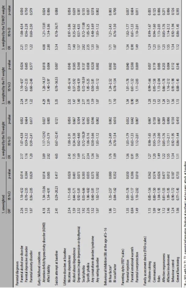
As a practical research example, we assessed the effect of using different statistical weights through data from the EDSP Study (Wittchen et al. 1998a, b; Lieb et al. 2000). The EDSP is a representative, prospective general population study on early phases of the development of mental and substance use disorders and their risk and vulnerability factors. The probands come from the city of Munich and its suburbs. Fig. 1 illustrates the design of the EDSP. Initially, the 14- to 15-year-old individuals at the baseline wave of assessment were sampled with twice the probability of the 16- to 21-year-olds, and the 22- to 24-year-olds were sampled at half this probability. In the present article, we focus on only 933 probands of the young cohort (14–17 years of age at baseline), whose biological mothers were interviewed. Among these mothers, parental diagnoses and parenting styles of education were assessed (among other variables not analysed in this paper). We examined the associations among a

variety of covariates and the new onset of panic attacks during the EDSP follow-up (T1/T2). Three weighting variables were created: (i) the T0 weight which adjusts the observed

marginal distributions of age, gender and geographic location among 1,395 individuals (14– 17 years old) at baseline to the distribution in the population of Greater Munich; (ii) the T1 weight which multiplies the T0 weight with the inverse T1/T0 ratios of the joint frequencies of sex, age and region (here Munich city vs. suburbs of Munich only) in 16 cells. For this purpose, 1,228 adolescents who had completed the first follow- up (T1) were used; and (iii) the T2-MOT weight which multiplies the T0 weight by the inverse T2- MOT/T0 ratios of the joint frequencies of sex and age in eight cells among 933 participants who had completed all three EDSP waves of assessment (T0, T1, T2) and whose biological mothers had been interviewed (MOT). Region was no longer considered because the drop-out rates (drop-out from 1,395 individuals at baseline to 933 in the final sample) were almost equal here (35.1% Munich city, 32.7% Munich suburbs; OR=0.91, 0.69–1.20, p=0.516, adjusted for eight cells of age and sex; weighted with the T0 weight). Diagnoses at baseline were not incorporated into the weighting variables because they were not predictive of drop-out from 1,395

individuals at baseline to 933 in the final sample (adjusted for age, gender and Munich city vs. suburbs with the T0 weight) or they had such a low prevalence that no major bias was

expected by disregarding them (i. e. dysthymia with 57.6% vs. 33.9% drop-out rate, OR=2.72, 1.36–5.45, and a prevalence of 2.3%; and agoraphobia w/o panic disorder with 59.7 vs. 33.7% drop-out rate, OR=2.94, 1.38–6.28, and a prevalence of 2.7 %). The standard deviation of the T0 weight is lowest with 0.39 and increases slightly to 0.40 for the T1 and to 0.45 for the T2-MOT weight. We obtained robust confidence intervals with the Huber- White sandwich estimator. All analyses were run with Stata 8 (Stata Corp. 2003). Of the 933 individuals, 30 were omitted from the analyses as they already had a panic attack at T0 leaving a total of 903 respondents for analyses. Table 1 contains the weighted and the unweighted results of the associations (adjusted for age and gender) of several predictors with incident panic attack at T1/T2 from separate logistic regressions. Whereas the point estimates were fairly equal across the three weights, there are some noteworthy discrepancies between the weighted and the unweighted results. The unweighted odds ratio of reporting a suicide attempt at baseline and panic attack later is 2.41 and rises at least to 4.65 in the weighted analyses. Although this odds ratio did not reach statistical significance in any of the models, a larger sample might have led to a different conclusion. Similar results were found for social phobia and the FAD (family assessment device) problem-solving and communication scales. A diagnosis of depression at baseline, on the other hand, yielded an unweighted estimate of 2.32, which was considerably higher than each of the weighted estimates (at most 1.69). In order to see which component of the weighting scheme was mainly responsible for these discrepancies, we analysed the

interactions of age, gender and location with the predictors and incidence of panic attacks (in separate models). With the T2-MOT weight, we found that the odds ratio of the FAD

communication scales increased with increasing age (OR for communication* age in years=1.28, 95% CI=1.04–1.58, main effect communication OR=0.01, 0.0002–0.54). The odds ratio for the behaviour control scale, however, varied by gender; the odds ratio of women was 1.78 times (1.00–3.14) that of men (OR for main effect of behaviour control= 0.90, 0.66–1.23). For the categorical prognostic factors, no significant interactions were found, and age and sex jointly contributed to the discrepancies. Regarding the results of the three weighting variables in Table 1, not only the point estimates, but also the confidence intervals, yielded quite similar results across the three weights, so that the kind of weight makes no difference in the present example. The latter finding is not surprising as the standard deviation was similar across the three weights.

In this article, we reviewed the major ideas on selection bias and the use of statistical weights to correct for different probabilities of sampling or participation. With data from the EDSP Study, we found that disregarding the different sampling rates according to age as well as non-response at baseline according to age, sex and location can have a considerable impact on point estimates of odds ratios. The particularity of the EDSP-Study is that the original sample was drawn with different sampling probabilities according to age. Because adolescence is assumed to be a crucial period in the development of mental disorders, interactions of risk factors with age can be assumed to be common here. In our example, we focussed only on data from the young cohort, 14–17 years old at baseline. In the whole sample of 14–24 years old at baseline, the bias introduced by the non-representative age distribution might be much stronger. Sampling bias, therefore, can have a major impact also on associations and not only on marginal distributions such as prevalence rates, although it is likely that more examples for the latter can be found. Using other measures of associations like the risk ratio and the risk difference can be assumed to increase the problem in the sense that the odds ratio tends to be the smoothest measure; that is, its use tends to require less interaction terms because they are related to logistic regressions (McCullagh and Nelder 1989). Examples, however, it can only suggest that weighting is necessary, not that it is unnecessary. They do not allow us to

demonstrate that the incorporation of specific variables into the weighting scheme is sufficient because other, more important factors, may be unobserved or unknown. The benefits of reducing bias (and the robustness against model-misspecification in regression models) should be balanced against the increase in variance. When designing a study participation probabilities should be maximized and as much information as possible should be collected about potential determinants of participation. Then, different weights can be created, and for each analysis, the accuracy of a weight should be balanced against the increase in variance. The best available weight is the one that is minimally sufficient, that is, another weight incorporating more information would hardly change the point estimate, but rather increase the variance.

Acknowledgements

This study is part of the Early Developmental Stages of Psychiatry (EDSP) Study and is funded by the German Ministry of Research and Technology, project no. 01 EB 9405/6 and 01 EB 9901/6 as well as by the Deutsche Forschungsgemeinschaft LA 1148/1-1. We wish to thank Evelyn Alvarenga for language editing.

References

1. Allehoff WH, Esser G, Schmidt MH, Hennicke K (1983) Die Bedeutung der Informations- und Kooperationsverweigerung für die Interpretationsreichweite einer mehrstufigen kinderpsychiatrisch- epidemiologischen Untersuchung. Soc Psychiatry 18: 29–36

2. Binder DA (1983) On the variances of asymptotically normal estimators from complex surveys. Int Stat Rev 51:279–292

3. Brogan DJ (1998) Pitfalls of using standard statistical software packages for sample survey data. In: Armitage P, Colton T (eds) Encyclopedia of Biostatistics, 4167–4174. New York: John Wiley and Sons

4. Carpenter J, Bithell J (2000) Bootstrap confidence intervals: when, which, what? A practical guide for statisticians. Stat Med 19:1141–1164 299

5. Cox DR, Wermuth N (1996) Multivariate dependencies, Chapman und Hall, London

6. Diggle PJ, Liang K-Y, Zeger SL (1994) Analysis of longitudinal data, Oxford University Press, Oxford

7. Efron B, Tibshirani RJ (1993) An introduction to the bootstrap, Chapman and Hall, London 8. Greenland S (1977) Response and follow-up bias in cohort studies. Am J Epidemiol 106:184–187 9. Greenland S (in press) Multiple-bias modeling for analysis of observational data. J Roy Stat Soc 10. Heeringa SG, Liu J (1998) Complex sample design effects and inference for mental health survey data. Int J Methods Psychiatr Res 7:56–65

11. Heyting A, Tolboom JTBM, Essers JGA (1992) Statistical handling of dropouts in longitudinal clinical trials. Stat Med 11: 2043–2061

12. Insightful Corp. (2003) Documentation for S-PLUS 6.2, Seattle, WA: Insightful Corp

13. Jacobi F, Wittchen HU, Holting C, Sommer S, Lieb R, Höfler M, Pfister H (2002) Estimating the prevalence of mental and somatic disorders in the community: aims and methods of the German National Health – Interview and Examination Survey. Int J Methods Psychiatr Res 11:1–18 14. Kauermann G, Carroll RJ (2001) A note on the efficiency of sandwich covariance matrix estimation. J Am Stat Ass 96:1387–1396

15. Kessler RC, McGonagle KA, Zhao S, Nelson CB, Hughes M, Eshleman S, Wittchen HU, Kendler KS (1994) Lifetime and 12-month prevalence of DSM-III-R psychiatric disorders in the United States: Results from the National Comorbidity Survey. Arch Gen Psychiatr 51:8–19

16. Kessler RC, Little RJA, Groves RM (1995) Advances in strategies for minimizing and adjusting for survey nonresponse. Epidem Rev 17:192–204

17. Kish L, Frankel MR (1970) Balanced repeated replications for standard errors. J Amer Stat Ass 65:1071–1095

18. Levy PS, Lemeshow S (1999) Sampling of populations – methods and application, John Wiley and Sons, New York

19. Lieb R, Isensee B, Von Sydow K, Wittchen HU (2000) The Early Developmental Stages of the Psychopathology Study (EDSP): A methodological update. Eur Add Res 6:170–182

20. Light RJ, Singer JD, Willett JB (1990) By design – planning research on higher education. Harvard University Press, Cambridge MA

21. Little RJA (1986) Survey nonresponse adjustments for estimates of means. Int Stat Rev 54:139– 157

22. Little RJA, Lewitzky S, Heeringa S, Lepkowski J, Kessler RC (1997) Assessment of weighted methodology for the national comorbidity survey. Am J Epidem 146:439–449

23. McCullagh P, Nelder JA (1989) Generalized Linear Models, 2nd _{edition. Chapman and Hall,}

24. Miller ME, Ten Have TR, Reboussin BA, Lohmann KK, Rejeski WJ (2001) A marginal model for analysing discrete outcomes from longitudinal surveys with outcomes subject to multiple-cause non-response. J Am Stat Ass 95:844–857 25. Pigeot I (2001) The jackknife and bootstrap in biomedical research – Common principles and possible pitfalls. Drug Information Journal 35:1431–1443

26. Preisser JS, Galecki AT, Lohmann KK, Wagenknecht LE (2000) Analysis of smoking trends with incomplete longitudinal binary responses. J Am Stat Ass 95:1021–1031

27. Rao JNK, Shao J (1999) Modified balanced repeated replication for complex survey data. Biometrika 86:403–415 28. Rotnitzky A, Robins J (1997) Analysis of semi-parametric regression models with non-ignorable non-response. Stat in Med 16:81–102

29. Rosenbaum PR (2002) Observational Studies, 2nd edition Springer, New York

30. Rosenbaum PR, Rubin DB (1983) The central role of the propensity score in observational studies for causal effects. Biometrika 70:41–55

31. Rubin DB (1996) Multiple imputation after 18+ years. J Amer Stat Ass 91:473–489 32. Rubin DB (2003) Discussion on multiple imputation. Int Stat Rev 71:619–625

33. Rubin DB, Schenker N (1991) Multiple imputation in health care databases: an overview and some applications. Stat Med 10:585–598

34. Royall RM (1986) Model robust confidence intervals using maximum likelihood estimators. Int Stat Rev 54:221–226

35. Schafer JL (1997) Analysis of incomplete multivariate data, Chapman and Hall, London 36. Scharfstein DO, Rotnitzky A, Robins JM (1999) Adjusting for nonignorable dropout using semiparametric nonresponse models. J Am Stat Ass 94:1096–1120

37. Smith TMF (2001) Biometrika Centenary: sample surveys. Biometrika 88:167–194 38. SAS Institute Inc. (2003) SAS OnlineDoc® 9.1. Cary, NC: SAS Institute Inc

39. Shah BV, Barnwell BG, Bieler GS (2004). SUDAAN User’s manual: Release 9.0, NC: Research Triangle Institute, Research Triangle Parc

40. SPSS Inc. (2004) SPSS for Windows Version 13. Chicago, IL: SPSS Inc

41. StataCorp. Stata Statistical Software: Release 8.0 (2003) College Station, TX: Stata Corporation 42. Touloumi G, Pocock SJ, Babiker AG, Darbyshire JH (2002) Impact of missing data due to selective dropouts in cohort studies and clinical trials. Epidem 13:347–355

43. Troxel AB, Lipsitz SR, Brennan TA (1997) Weighted estimation equations with nonignorably missing response data. Biometrics 53:857–869

44. White H (1982) Maximum likelihood estimation of misspecified models. Econometrica 50:1–25 45. Wittchen H, Höfler M, Gander F, Pfister H, Storz S, Üstün TB, Miller N, Kessler RC (1999) Screening for mental disorders: performance of the Composite International Diagnostic-Screener (CID-S). Int J Meth Psychiatr Res 8:59–70

46. Wittchen HU, Perkonigg A, Lachner G, Nelson CB (1998a) Early Developmental Stages of Psychopathology Study (EDSP): Objectives and design. Eur Add Res 4:18–27

47. Wittchen HU, Nelson CB, Lachner G (1988b) Prevalence of mental disorders and psychosocial impairments in adolescents and young adults. Psychol Med 28:109–126

48. Yung W, Rao JNK (2000) Jackknife variance estimation under imputation for estimators using poststratification information. J Am Stat Ass 903–915