A METHODOLOGY FOR MODELING A LARGE LOCATION PROBLEM
Samuel Vieira Conceição* Luís Henrique Capanema Pedrosa**
Marcellus Vinagre da Silva** Álvaro Simões da Conceição Neto** * Department of Industrial Engineering Federal University of Minas Gerais, Brazil Avenida Antonio Carlos, 6627 – Pampulha
CEP – 30161-010 Belo Horizonte - MG
** Cia. Siderúrgica Belgo-Mineira – Arcelor Group
ABSTRACT
In this work, we propose a methodology to collect and model a large data base of an existing distribution network and also how to prepare the input data set for a decision support system to solve a large location problem. We discuss how to accurately integrate information about transportation, logistics costs and customer service, sales forecast, production rate and plant capacity in order to solve a large location problem. The result was a well-designed set of essential and aggregated information validated by top management to be used as inputs of the location problem.
Keywords: location problem, data aggregation, supply chain optimization INTRODUCTION
Location problems have been discussed in the literature of operations research and management science since the early 60´s. Since then, many developments leaded for today’s capacity to solve the majority of real location problems. Only in recent years, the gathering and modeling of large data base became possible and consequently the large real systems could be optimized. The main purpose is to garantee that essential features of the real system must be reflect in sufficient detail to assure that the model will yield valid conclusions and earn the active acceptance of management.
Geoffrion and Powers (1995) point out the main factors that turned the application of large scale optimization on distribution planning technically feasible: The evolution of computers and communications technology; the evolution of data development and management tools; the evolution of model features and software capabilities; the evolution of algorithms; the evolution of logistics as a corporate function; the evolution of how companies actually use software for designing distribution systems.
The first two factors have a particular importance in this work. As the study were conducted in a very large steel company, with 7 plants, 13 distributions centers, more than 2,000 customers in 1,400 cities, all located in different parts of the country, and around 10,000 products (SKUs), without the development of the information technology and data management tools, real problems of such nature would remain unpractible.
One of the main contributions of the work is to show how a real distribution system can be modeled in its essential features as inputs of a location problem using a decision support system which integrates an ERP system.
BACKGROUND
As can be noticed in main surveys about location problems (Aikens, 1985; Brandeau and Chiu, 1989; Drezner, 1995; Owen and Daskin, 1998; Melkote and Daskin, 2001), most works in network design and facility location do not describe how data were collected and modeled. Usually, the concerns are about testing and refining the algorithms. Few authors point out how to model data for network distribution planning. Basically the data modeling activity for logistic models is to aggregate available data into categories to simplify the statement and the solution of the problem. Most authors focused three categories of data for aggregation: products, customers, and freights.
Products may be grouped from 3 to 30 product groups to reflect production and distribution conditions (Geoffrion et al., 1975). Its common to need no more than 20 product groups which may be classified into two broad categories: 1) products that are shipped directly in bulk to customers and 2) products that are shipped through warehouses (Ballou, 1998). Another way to group products is to take into account similar conditions of distribution, production and distribution channels (Bowersox and Closs, 2001). An aggregation by customer segment and production similarities was also employed to group 1500 products in 18 product groups by Shapiro (Shapiro et al., 1993).
Like products, customers may also be grouped to simplify the analysis and results. One of the main difficulties in aggregating customers is to define the quantity of groups or areas needed to obtain consistent results. Customer groups my be formed by geographical distribution or mode of shipment (TL vs. LTL) (Geoffrion et al., 1982), zip code (Shapiro et al., 1993; Ballou, 1998), city, estatistical zone (Bowersox and Closs, 2001), largest customers as separate demand points and aggregate the remaining customers on a geographical basis (Shapiro et al., 1993). The transportation cost errors in customer aggregation has been investigated by Ballou (Ballou, 1994) and the influence of customer grouping when demand is correlated with resource requirements was investigated by Tyagi and Das (Tyagi and Das, 1999).
Finally, aggregate freights are normally weighted averages reflecting the mix of modes and shipment sizes deemed likely to prevail (Geoffrion et al., 1982). The rates should be obtained for quantity and mode of transport and between distribution centers and customers (Bowersox and Closs, 2001).
DATA GATHERING AND MODELLING
One of the most important stages of any location problem is data gathering and modeling, since the validity of results is mostly dependent on the accuracy of the data input into the decision support system. Oversimplification has been responsible for a high proportion of the past failures of distribution planning models in terms of their actual decision-making impact (Geoffrion and Powers, 1995).
Data gathering
The data sources required for the distribution planning model are dispersed all over the distribution network. Data related to the real demand is considered only when products are shipped to customers, since orders may be cancelled. The demand data are gathered and centralized in the company´s data base.
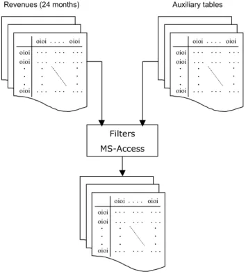
Thus, the first step to collect and model data from the distribution network was to extract a initial data set, the table of revenues over the last 24 months, structured as follows: Date of shipment; Plant of
the product shipped; Quantity shipped and Customer ID (code and name). It is important to point out that the size of data base extracted from the system was fairly large, containing more than 290,300 lines. Such a large amount of data was handled only by mainframes until recently. In addition, we used a set of auxiliary tables, more specifically the table of products, containing the description and code of each product and its associated product groups, and the table of customer groups, containing the cities with its codes and associated customer groups.
The auxiliary tables combined with the revenues table enabled us to extract quantitative information about the company´s network as listed below: Share of each region of the country in total revenues; Share of each state in total revenues; Quantity of each product group demanded in every customer group, state, region, etc.
Filters MS-Access oioi oioi oioi oioi oioi . . . . . . . . . . . . . . . . . . . . . . . . . . . . . . . . . . . . . . Revenues (24 months) oioi oioi oioi oioi oioi . . . . . . . . . . . . . . . . . . . . . . . . . . . . . . . . . . . . . . Auxiliary tables oioi oioi oioi oioi oioi . . . . . . . . . . . . . . . . . . . . . . . . . . . . . . . . . . . . . .
Structured information about the company´s network
Figure 1 – Process of obtaining structured information about the company´s network
Data modeling
Once modeled, essential features of the real system are the inputs of the decision support system (presented in the next section) and are listed below:
• Customers: more than 2,000 customers in 1,408 cities were grouped in 70 customer groups, based on geographical distribution and steel consumption. An index of consumption was created to reflect the steel demand per city. When the sum of consumption indexes from a group of cities reached a lower limit previously established, a customer group was formed. The number of customer groups per state follows exactly the demand profile of those states.
• Products: more than 10,000 products were grouped in 19 product groups according to their similarities in production process, plant of production and market segment.
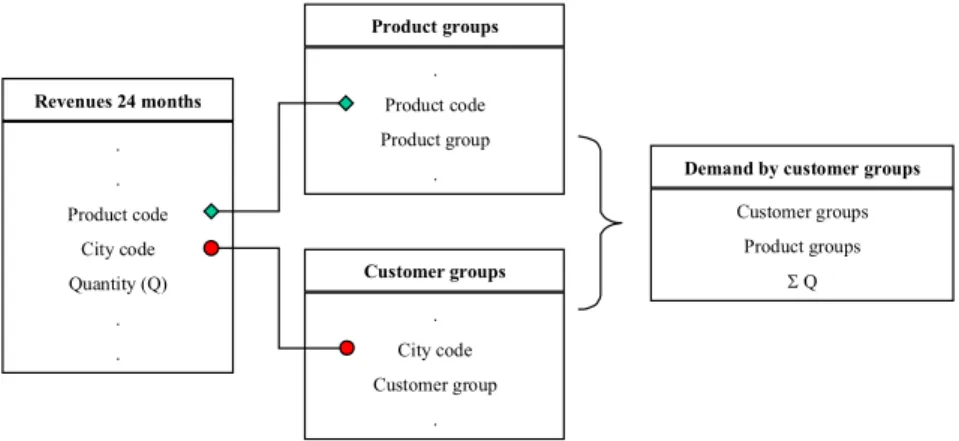
• Demand: the demand for each product group was calculated by adding up the demand for each product associated with each customer belonging to each customer group. Then, aggregating customers into customer groups and products into product groups generated a table of demand of product groups by customer groups.
. . Product code City code Quantity (Q) . . Revenues 24 months . Product code Product group . Product groups . City code Customer group . Customer groups Customer groups Product groups Σ Q
Demand by customer groups
Figure 2 – Process of obtaining the demand of product groups by each customer group.
• Freight rates: the freight rates from every origin point to every destination point (Cij) were
collected from the company´s data base and correspond to real values paid to carriers. As the
customers were grouped into customer groups, the average freight rate (CiR) for the group
(regarding the origin point) was calculated by summing up freight rates per customer weighted by
the demand (Qij) of that specific customer for products shipped from the considered origin point.
This procedure was repeated for all customer groups from all origin points.
• Distances: similar to the freight rates previously described, the distances from every origin point
to every destination point (Dij) were collected from the company´s data base. As the customers
were grouped into customer groups, the average travel distance (DiR) for the group (regarding the
origin point) was calculated by summing up travel distances per customer weighted by the
demand (Qij) of that specific customer for products shipped from the considered origin point.
This procedure was repeated for all customer groups from all origin points.
Plant DC Aggregated demand Customer group (R) CiR , DiR QR =
Σ
Qij Main city Plant DC Customer group (R) Main city- cities contained in the customer group
Cij , Dij
Qij
• Speed of transportation mode: we assumed that the maximum travel distance per day is 500 km for 8 hours journey. It was needed to use an equivalent speed for a 24 hours jorney to cover the same distance as the optimizer does not consider spare time. It uses the distance to calculate the duration of new transportation lanes and compare it to the required service level of the customer groups.
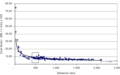
• Freight cost factor: freight cost factor is used for those lanes that are currently not used by the actual distribution network but may be assigned by the optimizer as a solution of the optimized network. The cost factor is expressed by $/ton/km and could be calculated dividing the freight rates ($/ton) by the distances (km) from every origin point to every customer group. The average value is the cost factor. For shorter distances (500 km), there is an increase of the influence of fixed costs in the total transportation costs. As the distance increases, such influence decreases as the variable costs prevail.
T ransportation Cost factor x Distance
y = 111,64x-0,4068 -10,00 20,00 30,00 40,00 50,00 60,00 70,00 80,00 - 500 1.000 1.500 2.000 2.500 Distance (km) C o s t fa ct o r ( R $ / t / k m ) x 1 0 0
Figure 4 – Transportation costs per distance.
• Production contraints: in the distribution network, the production of the products are constrained by plant. The following figure presents the map of production of the 19 product groups by the seven plants:
Product
groups Plant #1 Plant #2 Plant #3 Plant #4 Plant #5 Plant #6 Plant #7
1 X X X 2 X 3 X X 4 X 5 X X 6 X 7 X 8 X X X 9 X X 10 X X X X 11 X 12 X 13 X X 14 X 15 X 16 X 17 X X 18 X 19 X
Table1 – Map of production of the product groups by plants.
• Production resources and capacity: since we were dealing with agreggated information, we realized that assigning real resources and productivity to product groups would lead to inconsistent values. In order to avoid such errors, “ficticious” resources were created, one for each product group at each plant where it is produced. Then we calculated productivity dividing the total annual production of a product group in a plant by the available time (in hours) of one year production. The productivity calculated is expressed in tons/hr.
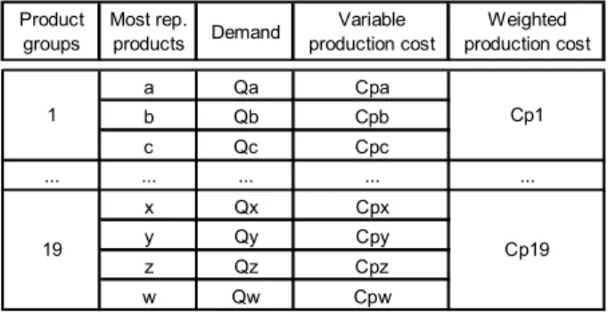
• Production costs: the production costs were collect from the company´s data base. A weighted average by demand were calculated for the production costs of the 70% most representative products of each product group.
Product groups Most rep. products Demand Variable production cost Weighted production cost a Qa Cpa b Qb Cpb c Qc Cpc ... ... ... ... ... x Qx Cpx y Qy Cpy z Qz Cpz w Qw Cpw 1 Cp1 19 Cp19
Table 2 – Weighted production cost by product group.
• Storage capacity: the values used correspond to the real condition of storage capacity in each distribution center. For the potential ones, the greatest values were considered.
• Inventory costs: The inventory costs were considered to be the cost of capital with an estimated monthly rate of 2%.
• Handling capacity: the values used correspond to the real condition of handling capacity in each distribution center. For the potential ones, the greatest values were considered.
• Handling costs: theses costs were calculated dividing the variable costs of the distribution centers by the quantity of product handled in and out of them. As these values seemed to be very similar from one DC to another, one single value was used for all of them, including the potential ones. • Openning costs: the openning costs of a new potential distribution center were estimated based on
costs incurred in the openning of the existing ones.
• Fixed and variable costs of the distribution centers: thoses costs were collect from the company´s data base. The costs of the plants and distribution centers were separated in fixed and variable. The costs for potential DCs were estimated based on the costs of existing ones.
• Penalty costs for delay and non-delivery: we defined very high values for penalties costs to eliminate this possibility in optimal solutions.
ERP SAP APO / Network Design
The APO/Network design is a decision support tool that integrates the ERP system SAP APO
set of possible new ones considering all relevant costs and capacity constraints. The result is an optimally reestructured network.
RESULTS
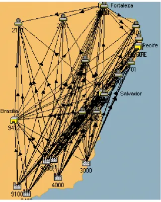
The following figure present part of the company´s distribution network with the essential elements of the Northeast of Brazil. The customers were aggregated in 12 customer groups and 3 DC´s are considered in the analysis. As we can see, even with the data aggregation, the problem is still complex and have many lanes, requiring optimization. We set the maximum deviation of 0,01% from optimality and got solutions within 3 minutes in a Pentium III, 1 GHz processor. The results are evaluated in Conceição et al. (2003).
Figure 5 – The distribution network of the Northeast of Brazil with its essential features.
CONCLUSIONS
In this paper, we sugested a methodology to aggregate and collect information about a large data base of an existing distribution network. In addition the methodology also pointed out how to prepare the input data set for a decision support system to solve a large location problem. We discussed how to accurately integrate information about transportation, logistics costs and customer service, sales forecast, production rate and plant capacity in order to solve a large location problem with 7 plants, 13 distributions centers, more than 2,000 customers in 1,400 cities, all located in different parts of the country, and around 10,000 products (SKUs.
A large amount of data was collected and modeled using desktop computers and comercial data management software. The degree and the quality of the data aggregation is determinant for the
Design was used as a decision support system to solve the problem and the results allowed us to validate the methodology and the system.
One of the main contributions of this work is to show how a real distribution system can be modeled in its essential features as inputs of a location problem using a decision support system which integrates an ERP system.
REFERENCES
Aikens, C. H. (1985), “Facility Location Models for Distribution Planning”, European Journal of
Operational Research, Vol. 22, pp.263-279.
Ballou, R. H. (1994), “Measuring Transport Costing Error in Customer Aggregation for Facilty
Location”, Transportation Journal, pp.49-59.
Ballou, R. H. (1998), Business Logistics Management, Prentice Hall, New Jersey.
Bowersox, D. J., Closs, D. J. (2001), Logística Empresarial: O Processo de Integração da Cadeia de
Suprimentos, Editora Atlas, São Paulo.
Brandeau, M. L., Chiu, S. S. (1989), “An Overview of Representative Problems in Location
Research”, Management Science, Vol. 35, No. 6, pp.645-674.
Conceição, S. V. et al. (2003). “Location Problem in the Steel Industry Using SAP APO/Network
Design Software as a Decision support system”, Euroma Poms International Conference 2003, Vol.
2, pp. 851-860.
Drezner, Z. (1995), Facility Location, Springer-Verlag, New York.
Geoffrion, A. M., Graves, G. W. (1974), “Multicommodity Distribution System Design by Benders
Decomposition”, Management Science, Vol. 20, No. 5, pp.822-844.
Geoffrion, A. M. (1975), “A Guide to Computer-Assisted Methods for Distribution Planning”, Sloan
Management Review.
Geoffrion, A. M., Graves, G. W., Lee, S.-J. (1982), “A Management Support System for Distribution
Planning”, Infor, Vol. 20, No. 4, pp.287-314.
Geoffrion, A. M., Powers, R. F. (1995), “Twenty Years of Strategic Distribution System Design: An
Evolutionary Perspective”, Interfaces, Vol. 25, No. 5, pp.105-127.
Melkote, S., Daskin, M. S. (2001), “Capacity Facility Location/Network Design Problems”, European
Journal of Operational Research, Vol. 129, pp.481-495
Owen, S. H., Daskin, M. S. (1998), “Strategic Facility Location: A Review”, European Journal of
Operational Research, Vol. 111, pp.423-447
Shapiro, J. F. (1993), “Optimizing the Value Chain”, Interfaces, Vol. 23, No. 2, pp.102-117.