STRATEGIES FOR FEATURE SELECTION IN
PREDICTIVE DATA MINING
by
Manjula Dissanayake
Submitted for the degree of
Doctor of Philosophy
Department of Computer Science
School of Mathematical and Computer Sciences
Heriot-Watt University
May 2015
The copyright in this thesis is owned by the author. Any quotation from the report or use of any of the information contained in it must acknowledge this report as the source of the quotation or information.
The improvements in Deoxyribonucleic Acid (DNA) microarray technology mean that thousands of genes can be profiled simultaneously in a quick and efficient man-ner. DNA microarrays are increasingly being used for prediction and early diagnosis in cancer treatment. Feature selection and classification play a pivotal role in this process. The correct identification of an informative subset of genes may directly lead to putative drug targets. These genes can also be used as an early diagnosis or predictive tool. However, the large number of features (many thousands) present in a typical dataset present a formidable barrier to feature selection efforts.
Many approaches have been presented in literature for feature selection in such datasets. Most of them use classical statistical approaches (e.g. correlation). Clas-sical statistical approaches, although fast, are incapable of detecting non-linear in-teractions between features of interest. By default, Evolutionary Algorithms (EAs) are capable of taking non-linear interactions into account. Therefore, EAs are very promising for feature selection in such datasets.
It has been shown that dimensionality reduction increases the efficiency of feature selection in large and noisy datasets such as DNA microarray data. The two-phase Evolutionary Algorithm/k-Nearest Neighbours (EA/k-NN) algorithm is a promising approach that carries out initial dimensionality reduction as well as feature selection and classification.
This thesis further investigates the two-phase EA/k-NN algorithm and also in-troduces an adaptive weights scheme for thek-Nearest Neighbours (k-NN) classifier. It also introduces a novel weighted centroid classification technique and a correla-tion guided mutacorrela-tion approach. Results show that the weighted centroid approach is capable of out-performing the EA/k-NN algorithm across five large biomedical datasets. It also identifies promising new areas of research that would complement the techniques introduced and investigated.
I am very grateful for the support that I received throughout this research. First of all, I would like to thank Professor David Corne for his continued guidance and encouragement. I always felt supported and confident under the supervision of Professor Corne. I would like to thank my parents for their ever-present support and for encouraging me to always pursue my academic goals. I would also like to thank my wife, Indy, for her patience and understanding throughout what has been a long process. Finally, I would like to thank the rest of my family and friends for their support, and my brother, Upul Dissanayaka, for helping to proofread this work.
1 Introduction 1
1.1 Introduction . . . 1
1.1.1 Feature Selection and Classification . . . 2
1.2 Two-Phase Evolutionary Algorithm/k-Nearest Neighbours Algorithm for Feature Selection and Classification . . . 3
1.3 Datasets . . . 4
1.3.1 Leukaemia Dataset . . . 4
1.3.2 Ovarian Cancer Dataset . . . 5
1.3.3 Prostate Cancer Dataset . . . 5
1.3.4 Breast Cancer Dataset . . . 5
1.3.5 Colon Cancer Dataset . . . 5
1.4 Contributions . . . 6
1.5 Publications Resulting From this Research . . . 7
1.6 Outline of Thesis . . . 7
2 Literature Review 9 2.1 Deoxyribonucleic Acid Microarrays . . . 9
2.2 Overview of Feature Selection and Classification Techniques . . . 10
2.2.1 Filter Techniques . . . 11
2.2.2 Wrapper Techniques . . . 11
2.2.3 Embedded Techniques . . . 13
2.2.4 Hybrid Techniques . . . 13
2.3 Evolutionary Algorithm/k-Nearest Neighbours Algorithm . . . 15
2.4 Two-Phase Evolutionary Algorithm/k-Nearest Neighbours Algorithm 16 2.4.1 Two-Phase Evolutionary Algorithm/k-Nearest Neighbours Al-gorithm Explained . . . 18
2.4.2.1 Phase One . . . 21
2.4.2.2 Phase Two . . . 23
2.4.3 Results from Two-Phase Evolutionary Algorithm/k-Nearest Neighbours Algorithm . . . 24
2.5 Multi-Objective Evolutionary Algorithms . . . 25
2.6 Related Results from Literature for the Datasets Used in This Thesis 28 2.6.1 Leukaemia Dataset . . . 28
2.6.2 Prostate Cancer Dataset . . . 32
2.6.3 Ovarian Cancer Dataset . . . 32
2.6.4 Colon Cancer Dataset . . . 32
2.6.5 Breast Cancer Dataset . . . 32
3 Study of Parameters and Multi-Objective Approach in Two-Phase Evolutionary Algorithm/k-Nearest Neighbours Algorithm 34 3.1 Algorithms . . . 35
3.1.1 Two-Phase Evolutionary Algorithm/k-Nearest Neighbours . . 35
3.1.2 Multi-Objective Two-Phase Evolutionary Algorithm/k-Nearest Neighbours . . . 39
3.2 Datasets . . . 41
3.3 Experiments . . . 42
3.3.1 Leukaemia Dataset . . . 42
3.3.1.1 Single Objective Two-Phase Evolutionary Algorithm/k -Nearest Neighbours . . . 42
3.3.1.2 Multi-Objective Two-Phase Evolutionary Algorithm/k -Nearest Neighbours . . . 44
3.3.2 Ovarian Cancer & Prostate Cancer Datasets . . . 44
3.4 Results & Discussion . . . 44
3.4.1 Initial Parameter Tuning: Chromosome Size . . . 44
3.4.2 Initial Parameter Tuning: The Effect of α . . . 46
3.4.2.1 Effect ofα on the Leukaemia Dataset . . . 51
3.4.2.2 Effect ofα on the Prostate Cancer Dataset . . . 51
3.5 Conclusion . . . 56
4 An Adaptive Weights Scheme for k-Nearest Neighbours in Evo-lutionary Algorithm/k-Nearest Neighbours Algorithm for Feature Selection 58 4.1 Introduction . . . 58
4.2 Improvements to the Methodology . . . 59
4.2.1 Cross-validation . . . 59
4.2.2 Model Selection . . . 60
4.2.3 Setting up of Phase I & II of the Two-Phase Evolutionary Algorithm/k-Nearest Neighbours Algorithm . . . 62
4.3 Adaptive Weights for k-Nearest Neighbours . . . 63
4.3.1 Adaptive Weights for k-Nearest Neighbours Explained . . . . 64
4.3.2 Application of Adaptive Weights . . . 65
4.4 Algorithms . . . 67
4.4.1 Stand-alone k-Nearest Neighbours and Weighted k-Nearest Neighbour . . . 67
4.4.2 Single-objective Evolutionary Algorithm/k-Nearest Neighbours Algorithm . . . 68
4.4.3 Single-objective Evolutionary Algorithm/Weighted-k-Nearest Neighbours Algorithm . . . 68
4.4.4 Single-objective Evolutionary Algorithm/Weighted Centroid Classification Algorithm . . . 69
4.5 Preliminary Experiments . . . 70
4.5.1 Speed of the Algorithm . . . 70
4.5.2 Estimating T . . . 72
4.6 Main Experiments . . . 73
4.6.1 Set-up of the Two-Phase Evolutionary Algorithm/k-Nearest Neighbours Algorithm . . . 73
4.6.2 Exploration of Feature Weights . . . 74
4.7 Results and Discussion . . . 74
4.7.2.1 Stand-alone k-NN and W-k-NN on the Leukaemia
Dataset . . . 75
4.7.2.2 Stand-alone k-Nearest Neighbours and Weighted k -Nearest Neighbour on the Prostate Cancer Dataset . 76 4.7.2.3 Stand-alone k-Nearest Neighbours and Weighted k -Nearest Neighbour on the Ovarian Cancer Dataset . 76 4.7.3 Two-Phase Evolutionary Algorithm/k-Nearest Neighbours vs. Two-Phase Evolutionary Algorithm/Weighted-k-Nearest Neigh-bours . . . 77
4.7.3.1 End-Point Experiments for Phase I . . . 78
4.7.4 The Set-Up of the Two-Phase Evolutionary Algorithm/k-Nearest Neighbours Algorithm Using the Method Proposed in 4.7.3.1 . 82 4.7.5 Application of Feature Weights . . . 88
4.7.6 Conclusion . . . 94
5 Correlation Guided Evolutionary Algorithm/k-Nearest Neighbours for Feature Selection 97 5.1 Introduction . . . 97
5.2 Overview of the Algorithm . . . 100
5.3 Correlation Guided Mutation . . . 101
5.3.1 Correlation Guided Mutation - Remove a Gene . . . 102
5.3.1.1 Preference Towards Selecting Strongly Correlated Fea-tures . . . 102
5.3.1.2 Preference Towards Selecting Loosely Correlated Fea-tures . . . 103
5.3.2 Correlation Guided Mutation - Add a Gene . . . 103
5.3.2.1 Preference Towards Selecting Strongly Correlated Fea-tures . . . 103
5.3.2.2 Preference Towards Selecting Loosely Correlated Fea-tures . . . 103
5.3.3.2 Preference Towards Selecting Loosely Correlated
Fea-tures . . . 104
5.4 Calculation of the Correlation Coefficient Matrix . . . 105
5.5 Biased Random Number Generation . . . 106
5.6 Experiment Set-up . . . 108
5.7 Results and Discussion . . . 109
5.8 Conclusion . . . 111
6 Conclusions and Future Work 117 6.1 Main Findings . . . 117
6.1.1 Parameters and Multi-Objective Approach in Two-Phase Evo-lutionary Algorithm/k-Nearest Neighbours Algorithm . . . 117
6.1.2 An Adaptive Weights Scheme for k-Nearest Neighbours in Evolutionary Algorithm/k-Nearest Neighbours Algorithm for Feature Selection . . . 118
6.1.3 Correlation Guided Evolutionary Algorithm/k-Nearest Neigh-bours for Feature Selection . . . 119
6.2 Future Work . . . 120
6.2.1 Setting up of the Two-Phase Evolutionary Algorithm/k-Nearest Neighbours Algorithm . . . 120
6.2.2 Multi-objective Approach . . . 121
6.2.3 Adaptive Weights . . . 121
6.2.4 Correlation Guided Mutation for Evolutionary Algorithm/k -Nearest Neighbours Algorithm . . . 123
6.3 Final Thoughts . . . 124
2.1 Summary of results for various approaches to feature selection and
classification in prostate cancer dataset. . . 26
2.2 Some well known multi-objective Genetic Algorithms adapted from Konak et al. [1] - part I. . . 29
2.3 Some well known multi-objective Genetic Algorithms adapted from Konak et al. [1] - part II. . . 30
2.4 Some well known multi-objective Genetic Algorithms adapted from Konak et al. [1] - part III. . . 31
2.5 Breast cancer dataset results by Sardana et al. [69]. The best per-forming classification method for each cross-validation technique is highlighted in bold face. . . 32
3.1 Effect ofα on the objective function . . . 42
3.2 Experiments run on the leukaemia dataset . . . 43
4.1 Sample Dataset . . . 66
4.2 Centroids . . . 66
4.3 Calculating everything on the fly vs. look up for k-Nearest Neighbours 75 4.4 Results from the application of feature weights to the Evolutionary Algorithm/k-Nearest Neighbours algorithm. . . 89
4.5 Results from the Evolutionary Algorithm/Weighted Centroid Classi-fication algorithm. . . 89
4.6 Baseline results to compare the two weighted algorithms against. . . . 89
4.7 Analysis of the various ways to set-up the two-phase Evolutionary Algorithm/k-Nearest Neighbours algorithm using Analysis Of Vari-ance. Please refer to 4.7.4 for an explanation of each method shown in this table. . . 90
Neighbours algorithm across five datasets. . . 91 4.9 Mean chromosome length and Standard Deviation for different ways
of setting up the two-phase Evolutionary Algorithm/k-Nearest Neigh-bours algorithm across five datasets. . . 92 4.10 Descriptives statistics on the results of various ways of setting up the
two-phase Evolutionary Algorithm/k-Nearest Neighbours algorithm across five datasets. . . 93 4.11 Calculation of mean ranks for each method of setting up two-phase
Evolutionary Algorithm/k-Nearest Neighbours algorithm. . . 95
5.1 An artificial dataset for illustrating the calculation of mean correla-tion coefficient for each feature. This dataset contains seven samples (S1 - S7). Each sample has six features F1 - F6). . . 102 5.2 Correlation coefficient matrix and the mean correlation coefficients
for each feature for the dataset shown in 5.1. . . 102 5.3 Overall results for correlation guided mutation with preference for
strongly correlated feature subsets for the Evolutionary Algorithm/k -Nearest Neighbours algorithm. . . 112 5.4 Overall results for correlation guided mutation approach with
prefer-ence for loosely correlated feature subsets for the Evolutionary Algorithm/k -Nearest Neighbours algorithm. . . 113 5.5 Overall results for correlation guided mutation approach with
pref-erence for strongly correlated feature subsets for Evolutionary Algo-rithm/Weighted Centroid Classifier algorithm. . . 114 5.6 Comparison of correlation guided mutation approaches to other
ap-proaches used in this thesis. The best algorithm for each dataset is highlighted in boldface. . . 115
6.1 The best results from all the algorithms tested in this thesis. The best algorithm for each dataset is highlighted in boldface. . . 125
2.1 A Deoxyribonucleic Acid microarray (adapted from http://en.wikipedia.org/wiki/DNA microarray) 9 2.2 Taxonomy of feature selection techniques adapted from [68]. . . 12
2.3 Support Vector Machine (SVM) applied to the leukaemia dataset. Fig-ure showing the application of the Support Vector Machine approach to the leukaemia dataset. Samples indicated by hollow triangle and rectangles are clos-est to the hyperplane and are therefore misclassified by the Support Vector Ma-chine [80]. . . 14 2.4 k-Nearest Neighbours (k-NN) Technique. Figure illustrating k-Nearest
Neighbours technique. Unknown type is classified as Type X using three closest neighbours. . . 15 2.5 Feature selection using an integer encoded chromosome. a) An
ex-ample of a dataset that has 3 sex-amples with 6 features in each sex-ample. b) An integer encoded chromosome that encodes 3 features. c) The dataset after it has been reduced in size using the chromosome. . . . 19
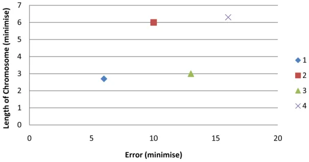
3.1 The concept of dominated solutions. Solution 1 is non-dominated as solutions 2, 3 & 4 are worse than solution 1 on both objectives. Solutions 2 & 3 do not dominate each other as solution 2 is better than 3 on accuracy but solution 3 is better on length. Both 2 & 3 are dominated by solution 1. Solution 4 is dominated by solutions 1, 2 & 3. 41
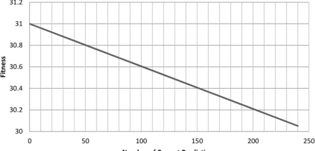
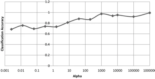
populated chromosomes decreases as the size of the chromosome is increased. This corresponds to an increase in the classification per-formance of these chromosomes. The value of the objective function during training stays low initially but increases as the size of the chromosome is increased corresponding to a degrading classification accuracy. The value of the objective function during testing follows the same trend as training albeit with markedly worse values due to over-fitting. . . 45 3.3 The effect of initial chromosome size on 3-fold cross-validated values
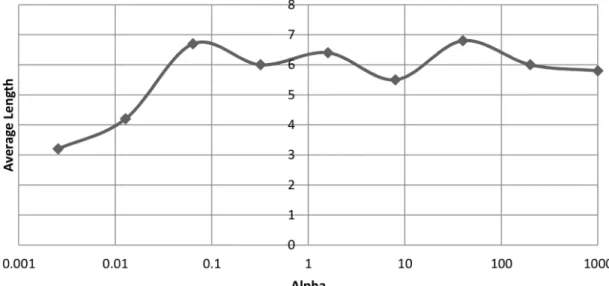
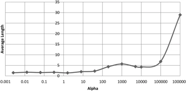
of the objective function. Average cross-validated objective function values of chromosomes versus the initial size of the chromosome. . . . 47 3.4 The effect of α on the final length of chromosomes after 2000
gener-ations. . . 47 3.5 Theoretical values produced by Equation 3.2 when the length of the
chromosome is 30 and α is 1. . . 48 3.6 Theoretical values produced by Equation 3.2 when the length of the
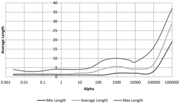
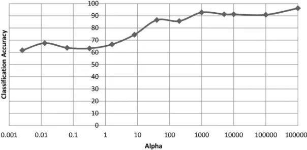
chromosome is 30 and α is 10, and when α is 1. . . 49 3.7 The effect that α has on final chromosomes on the ovarian cancer
dataset after 2000 generations. . . 49 3.8 The effect thatα has on the minimum, maximum and average length
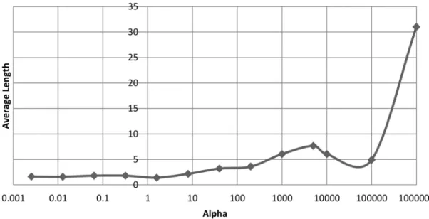
of final chromosomes on the ovarian cancer dataset after 2000 gener-ations. . . 50 3.9 The effect that α has on the average length of chromosomes on the
leukaemia dataset after 2000 generations. . . 51 3.10 The effect that αhas on the classification accuracy on the leukaemia
dataset after 2000 generations. . . 52 3.11 The effect that α has on the average length of chromosomes on the
prostate cancer dataset after 2000 generations. . . 52 3.12 The effect that α has on the classification accuracy on the prostate
cancer dataset after 2000 generations. . . 53 3.13 Best validated solutions for each experiment on the leukaemia dataset 53
3.15 Best validated solutions for each experiment on the prostate cancer dataset . . . 55
4.1 Accuracy of stand-alonek-Nearest Neighbours on the leukaemia dataset for a range of values for T. . . 75 4.2 Accuracy of stand-alone Weightedk-Nearest Neighbour on the prostate
cancer dataset for a range of values for T . . . 76 4.3 Accuracy of stand-alone Weightedk-Nearest Neighbour on the
ovar-ian cancer dataset for a range of values for T . . . 77 4.4 Leukaemia dataset: classification accuracy and chromosome length
vs. number of generations. The value of the objective function was calculated taking the length of the chromosome into account and Binary Tournament Selection was used as the selection method. . . . 80 4.5 Leukaemia dataset: classification accuracy and chromosome length
vs. number of generations. The value of the objective function was calculated without taking the length of the chromosome into account and Binary Tournament Selection was used as the selection method. . 81 4.6 Leukaemia dataset: classification accuracy and chromosome length
vs. number of generations. The value of the objective function was calculated taking the length of the chromosome into account and Rank Based Selection was used as the selection method. . . 82 4.7 Leukaemia dataset: classification accuracy and chromosome length
vs. number of generations. The value of the objective function was calculated without taking the length of the chromosome into account and Rank Based Selection was used as the selection method. . . 83 4.8 Ovarian cancer dataset: classification accuracy and chromosome length
vs. number of generations. The value of the objective function was calculated taking the length of the chromosome into account and Bi-nary Tournament Selection was used as the selection method. . . 84
calculated taking the length of the chromosome into account and
Bi-nary Tournament Selection was used as the selection method. . . 85
4.10 The probability of a mean rank happening by random chance. . . 88
4.11 Comparison of the baseline method vs. weighted methods. . . 94
5.1 Frequency of 10000 biased random numbers with abias of 0.5. . . 107
k-NN k-Nearest Neighbours.
ALH Adaptive Local Hyperplane.
ALL Acute Lymphoblastic Leukaemia.
AML Acute Myeloid Leukaemia.
ANN Adaptive Nearest Neighbour.
ANOVA Analysis Of Variance.
BTS Binary Tournament Selection.
cDNA complementary Deoxyribonucleic Acid.
cRNA complementary Ribonucleic Acid.
DMOEA Dynamic Multi-Objective Evolutionary Algorithm.
DNA Deoxyribonucleic Acid.
EA Evolutionary Algorithm.
EA/k-NN Evolutionary Algorithm/k-Nearest Neighbours.
EA/W-k-NN Evolutionary Algorithm/Weighted-k-Nearest Neighbours.
FS Feature Selection.
GA Genetic Algorithm.
JVM Java Virtual Machine.
KSVM k-Nearest Neighbours & Support Vector Machine Classifier.
LDC Linear Discriminant Classifier.
LOOCV Leave One Out Cross Validation.
MOEA Multi-Objective Evolutionary Algorithm.
MOGA Multi-Objective Genetic Algorithm.
MOP Multi-objective Optimisation Problem.
mRMR minimum Redundancy and Maximum Relevance.
NPGA Niched Pareto Genetic Algorithm.
NSGA Nondominated Sorting Genetic Algorithm.
NSGA-II Nondominated Sorting Genetic Algorithm-II.
PAES Pareto Archived Evolution Strategy.
PESA Pareto Envelope-based Selection Algorithm.
RAM Random Access Memory.
RBS Rank Based Selection.
RDGA Rank Density-based Genetic Algorithm.
RFE Recursive Feature Elimination.
RWGA Random Weighted Genetic Algorithm.
S2N Signal-to-Noise Metric.
SD Standard Deviation.
SPEA-2 Strength Pareto Evolutionary Algorithm-2.
SVM Support Vector Machine.
VEGA Vector Evaluated Genetic Algorithm.
W-k-NN Weighted k-Nearest Neighbour.
Introduction
1.1
Introduction
Recent advances in technology have tremendously increased humankind’s ability to create, store and carry out computations on digital data. It is estimated that in 2007, humankind had the capacity to store 44716 MB of optimally compressed data [29] per capita. In 1986, this figure was 539 MB [29]. This represents roughly an 83-fold increase in the per capita capacity to store data. Humankind’s capacity for carrying out computations on digital data has seen an even bigger increase. Hilbert et al. [29] estimated that in 1986, humankind had the per capita capacity to carry out 0.06 Mega Instructions Per Second (MIPS) on general purpose computers. By 2007, this figure had increased to 968 MIPS. In other words, this represents roughly a 16133-fold increase in the per capita capacity to carry out computations using general purpose computers in 21 years (1986 to 2007).
This explosion in both storage and computational capacity together with other scientific and technological advances has inevitably led to large scientific datasets. This is especially the case in the biomedical field. Recent advances in technologies such as high density Deoxyribonucleic Acid (DNA) microarrays and Proteomic anal-ysis has led to modern biomedical datasets that are usually rich in features. For example, the ovarian cancer dataset introduced by Petricoin et al. [61] has 15154 attributes (features) per sample. It is believed that only a handful of features are significantly differently expressed in a disease sample compared to a normal sam-ple. This means that data from DNA microarrays or Proteomic analysis is highly redundant and contain high dimensional noise [38, 46].
These datasets are valuable in that they have the potential to help us under-stand the pathology of certain diseases. A deeper underunder-standing of the pathology of diseases will help us deal better with these diseases. Another use of these datasets is that machine learning can be used to create models that help us in early diagnosis of certain diseases. However, the number of features present in a typical bioscience dataset presents a formidable barrier to such efforts.
This and other challenges associated with extracting high-level knowledge from real life large datasets has led to the emergence of the field of predictive data min-ing [79]. In this context, the aim of Feature Selection (FS) is to eliminate features that seem irrelevant to the case under study. FS on a feature-rich dataset results in a much reduced dataset. Predictive data mining can then perform faster with increased accuracy on these reduced datasets.
FS is in itself a rich area of research, and many of the techniques in this area rely on the use of statistical correlation measures to rank the features. However, though a convenient and fast approach to FS and very often used, statistical ranking based FS can be unwise; such methods will miss non-linear interactions between features, which in turn may be common in many datasets of interest.
1.1.1
Feature Selection and Classification
In predictive data mining, a model can be created that consists of a subset of features of the original dataset. In case of gene expression data related to a certain disease (e.g. cancer), it is possible that this subset of features can then be used as a predictor in unseen samples leading to early diagnosis. Therefore, FS is a technique commonly used in predictive data mining for building robust learning models that can be used to classify hitherto unseen data.
As the number of profiled features increase, the number of possible feature sub-sets that may be of importance grow exponentially. This makes the use of exhaustive search for FS infeasible.
This leaves heuristic search techniques such as Evolutionary Algorithms (EAs) as prime candidates for selecting feature subsets that are capable of discriminating between disease and normal cases [38, 50]. Many researchers are concentrating their efforts on methods that combine advanced search techniques (e.g. EAs) together with efficient classification techniques (e.g. k-Nearest Neighbours (k-NN)) for feature
selection and classification [38].
The most important objectives of feature selection are [68]:
• to avoid over-fitting and improve model performance, i.e. prediction perfor-mance of selected feature subset on unseen data.
• to provide faster and more cost-effective models.
• to gain a deeper insight into the underlying processes that generated the data.
1.2
Two-Phase Evolutionary Algorithm/
k
-Nearest
Neighbours Algorithm for Feature Selection
and Classification
Juliusdottir et al. [38] has introduced a two-phase Evolutionary Algorithm/k-Nearest Neighbours (EA/k-NN) algorithm for FS and classification in DNA microarray datasets that is capable of achieving comparable, if not better results, compared to other methodologies.
The two-phase EA/k-NN algorithm runs the EA/k-NN algorithm as both the prior-selection stage (on the complete dataset) and machine learning stage (on a reduced dataset). The EA used in the EA/k-NN algorithm is a generational, elitist EA that uses k-NN as the classifier/objective function. In the objective function, the classification error and the length of the chromosome are combined together to form a single metric that is minimised.
They argue that the use of k-NN as a classifier puts the onus on the search technique to find salient and significant gene subsets. Therefore, the two-phase EA/k-NN algorithm is capable of finding significant gene subsets which may have been overlooked with a more efficient classifier than k-NN.
Another advantage of using the EA/k-NN algorithm for initial feature selection (phase one) is that owing to generally good classification performance of k-NN, we can be confident that a good subset of features are selected. In other words, the chances of discarding a significant gene or a set of significant genes is lower when using this method compared to other methods.
Their two-phase EA/k-NN algorithm has led directly to the identification of three genes for prostate cancer and five genes for colon cancer. This supports previous
studies and further strengthens findings from those studies and suggests good targets for further research by domain experts.
Furthermore, two-phase EA/k-NN algorithm is relatively straightforward to im-plement and runs at an acceptable speed for even large datasets. However, there are areas in which the two-phase EA/k-NN algorithm could be better optimised and configured. Therefore, it was decided that this thesis would consist of a thor-ough investigation of the two-phase EA/k-NN algorithm as a candidate for FS and classification in predictive data mining in large biomedical datasets.
In particular, this thesis investigated the optimal way to set up the two-phase EA/k -NN algorithm so that it performs well across multiple datasets. This included an investigation into the population size, initial chromosome size, the balance between classification accuracy and the length of the chromosome in the objective function, number of generations to run phase one and phase two of the algorithm for and different ways in which genes can be selected during phase one that can then form the starting point of phase two. As an alternative to tuning some of the parameters of the algorithm (e.g. the balance between classification accuracy and the length of the chromosome in the objective function), an investigation into a multi-objective two-phase EA/k-NN was also carried out.
1.3
Datasets
1.3.1
Leukaemia Dataset
This is a publicly available dataset introduced by Golub et al. [22]. Their initial leukaemia dataset consisted of 38 bone marrow samples (27 Acute Lymphoblastic Leukaemia (ALL) samples & 11 Acute Myeloid Leukaemia (AML) samples) each containing 7070 genes. They tested their results on an independent dataset that had 34 samples (20 ALL, 14 AML).
These two datasets were mixed together to form a single dataset that had 72 samples out of which 47 samples were ALL and 25 samples were AML. The challenge with this dataset is to build models that can effectively classify a sample as either ALL or AML.
1.3.2
Ovarian Cancer Dataset
The ovarian cancer dataset is a publicly available dataset (Proteomic analysis data) introduced by Petricoin et al. [61]. This dataset contains 253 samples of which 91 are normal and 162 are cancer. Each sample contains 15154 values (features or genes). The aim of predictive data mining in this case is to classify unseen samples either as cancer or normal.
1.3.3
Prostate Cancer Dataset
This dataset was introduced by Singh et al. [72]. It contains 52 tumour and 50 normal samples with 12600 features per sample. As with the ovarian cancer dataset, the aim in this case is to predict whether an unseen sample is a cancer sample or normal sample.
1.3.4
Breast Cancer Dataset
The breast cancer dataset was introduced by Van’t Veer et al. [77] in patient outcome prediction for breast cancer. The original dataset was divided into training and test datasets. For the purpose of this thesis, both training and test datasets were mixed together to form one dataset that was then randomly split into smaller datasets as required. The complete dataset contains 46 samples of “relapse” cases and 51 “non-relapse” samples. Each sample contains 24481 genes. The aim of predictive data mining in this case is to predict the patient outcome as either “relapse” or “non-relapse”.
1.3.5
Colon Cancer Dataset
This dataset contains 62 samples collected from colon cancer patients and was in-troduced by Alon et al. [2]. It contains 40 tumour samples and 22 normal samples taken from a healthy part of the colon from the same patients. Each sample contains 2000 genes.
In their original study, Alon et al. [2] studied gene expression patterns using Affymetrix oligonucleotide arrays complementary to more than 6500 genes. How-ever, they then selected 2000 genes based on the confidence levels of the measurments of gene expression and used only these 2000 genes in their final analysis. Therefore,
it was decided to use the same 2000 genes in this thesis. The aim of predictive data mining in this case is to predictively discriminate between tumour and healthy samples.
1.4
Contributions
The following is a list of contributions made by this thesis to the field of FS and classification in predictive data mining. In particular, this thesis deals with large biomedical datasets.
• Juliusdottir et al. [38] introduced a novel two-phase EA/k-NN algorithm for FS and classification in DNA microarray datasets. The first contribution of this thesis is the investigation of the setting up of the two phases in the two-phase EA/k-NN algorithm including the parameters that needed to be tuned. This investigation was based on the hypothesis that phase one of the algorithm is critical to the success of the algorithm as only the genes selected during phase one are used for model building in phase two. The investigation revealed that some of the parameters need to be tuned correctly for each dataset for the algorithm to perform as described by Juliusdottir et al. [38].
• As an alternative to tuning parameters, a multi-objective EA was proposed in this thesis that could replace the single objective EA in the two-phase EA/k-NN algorithm. The multi-objective algorithm simultaneously optimises both the length of the chromosome (the number of features in the selected subset) and the classification accuracy without requiring a pre-tuned parame-ter labelled α. The multi-objective approach yielded very competitive results compared to the two-phase EA/k-NN algorithm.
• An investigation was carried into applying adaptive weights (adopted from Yang and Kecman [81]) to thek-NN algorithm in order to determine if weighted k-NN (Weighted k-Nearest Neighbour (W-k-NN)) would lead to discovery of optimal feature subsets. As withαin the single objective two-phase EA/k-NN algorithm, there are a few parameters that needs to be pre-tuned for W-k-NN to perform as expected. This thesis contributes that, with proper tuning, W-k-NN is able to out-performk-NN.
• Another contribution made by this thesis is the introduction of a novel weighted centroid classification technique as the objective function for the EA in the combined EA/k-NN approach. With this classification technique, the EA weighted centroid classification algorithm is able to out-perform both the EA/k-NN algorithm and the Evolutionary Algorithm/Weighted-k-Nearest Neigh-bours (EA/W-k-NN) algorithm.
• Classical statistical techniques (e.g. Analysis Of Variance (ANOVA)) were found to be ineffective at comparing multiple algorithms across multiple datasets in order to determine the best algorithm across all the datasets. In order to overcome this problem, a randomisation statistics approach was investigated and adopted in this thesis.
• Finally, this thesis introduces a correlation guided mutation operator. This mutation operator is designed towards selecting highly correlated features with a higher probability of being included in the chromosome. The results indicate this technique to be a promising technique for FS and classification.
1.5
Publications Resulting From this Research
Manjula SB Dissanayake and David W Corne. Feature selection and classification in bioscience/medical datasets: Study of parameters and multi-objective approach in two-phase EA/k-NN method. Computational Intelligence (UKCI), 2010 UK Work-shop on. IEEE, 2010.
1.6
Outline of Thesis
This thesis is organised as follows:
• Chapter 2 provides a review of FS and classification techniques found in liter-ature. It pays particular attention to FS techniques for DNA microarray data. It also contains a detailed introduction to the two-phase EA/k-NN algorithm and the adaptive weights scheme.
• Chapter 3 presents a detailed investigation into the configuration of the two phases of the two-phase EA/k-NN algorithm. It also presents an investigation into a multi-objective approach for FS and classification.
• Chapter 4 takes the investigation of the two phases started in Chapter 3 fur-ther. This chapter also introduces an adaptive weights scheme fork-NN algo-rithm and a novel weighted centroid classification technique.
• Chapter 5 provides an investigation into a novel correlation guided mutation operator for the EA/k-NN algorithm.
• Chapter 6 then presents a summary of the conclusions made in this thesis and presents a discussion of promising areas of further research.
Literature Review
2.1
Deoxyribonucleic Acid Microarrays
DNA microarrays, shown in Figure 2.1, are a relatively new, sophisticated technology used in molecular biology and medicine. They were first introduced in 1994 by Pease et al. [59].
Figure 2.1: A Deoxyribonucleic Acid microarray (adapted from http://en.wikipedia.org/wiki/DNA microarray)
Each DNA microarray consists of thousands of microscopic wells of DNA oligonu-cleotides arranged into a two-dimensional (2D) array shape. Each well contains pi-comoles of a specific DNA sequence. These wells in a DNA microarray are called features.
Each feature is capable of binding its corresponding complementary Deoxyri-bonucleic Acid (cDNA) or complementary RiDeoxyri-bonucleic Acid (cRNA) sequences. These cDNA or cRNA sequences are called targets. Targets are labelled with fluo-rophores or luminescence chemicals. It is possible to measure the amount of a target bound to each feature by measuring the amount of fluorescence [37].
DNA microarrays can be used to measure changes in expression levels of many thousands of genes simultaneously. This ability makes them a very powerful tool that can be used in early diagnosis and treatment discovery for many diseases [38]. The standard method for isolating genes responsible for a certain disease (e.g. cancer) is to measure gene expression levels of a number of patients (e.g. a couple of hundred) and compare them with expression levels of the normal population. As each chip is capable of monitoring many thousands of genes at one time and as the data collected from these experiments tend to be very noisy, this opens up a new challenge for computer scientists: feature selection and classification [38].
Typically, a microarray dataset consists of many thousands of genes but rela-tively few samples (a couple of hundred). This means that there may be many subsets of genes with good classification performance. The aim of feature selection and classification is to find as many near-optimal solutions as possible. The most frequently selected genes in these subsets can then be studied further as they have a better chance of being significant to the case under study [48].
2.2
Overview of Feature Selection and
Classifica-tion Techniques
As explained in 1.1.1, exhaustive searches for subsets of interesting features become infeasible as datasets get larger. This is due to the fact that if the original dataset contained N number of features, then the total number of possible feature sub-sets is 2N [13]. Therefore, even for relatively small datasets, complete or exhaustive
search for the optimal feature subset becomes infeasible. This leaves heuristic search techniques such as EAs as prime candidates for selecting feature subsets that are ca-pable of discriminating between disease and normal cases [38, 50] in large biomedical datasets.
Feature selection can be divided into supervised learning (e.g. classification where the class value is known in advance) and unsupervised learning (e.g. cluster-ing) [68]. As this thesis studies feature selection and classification in large biological datasets where the training data always contain class values, the appropriate learn-ing method for feature selection for this thesis is supervised learnlearn-ing.
is shown in Figure 2.2. Feature selection and classification techniques can be divided into four categories [68]:
• Filter
• Wrapper
• Embedded
• Hybrid
2.2.1
Filter Techniques
These techniques work by looking at the intrinsic properties of the dataset. For example, in most cases, a feature relevance score is calculated and low scoring fea-tures are pruned. The remainder of the dataset is then used for classification. The advantages of these techniques are that they can be easily scaled up or down, they are computationally simple and they are fast.
However, there are many disadvantages to this approach. For example, these techniques prune the dataset by looking at one feature at a time. This means that inter-feature relationships are not taken into account.
A number of multivariate filter techniques (e.g. Markov blanket filter) have been introduced in order to address some of the issues associated with univariate filter techniques [68].
Clustering analysis is also widely used with microarray data [2] for feature selec-tion and classificaselec-tion. Clustering analysis works by looking at correlaselec-tion between groups of genes and provides insight into gene-gene interaction. However, clustering analysis is not well suited for classification as it looks at correlated patterns of ex-pression rather than patterns of exex-pression that can differentiate between samples. It is also difficult to determine the relative importance of genes by using clustering analysis [48].
2.2.2
Wrapper Techniques
In wrapper techniques, a search procedure is defined that is capable of searching through the space of possible feature subsets for a given dataset. The search pro-cedure generates various subsets of features and they are evaluated against a test
Figure 2.2: T axonom y of feature selection tec hniques adapt ed from [68 ].
set by the classification algorithm [38, 68]. Therefore these techniques are tailored to whatever the classification algorithm that is used in the evaluation. Wrapper techniques are able to take inter-feature relations into account. However, they can be very computationally expensive, especially if the classification step is computa-tionally heavy [68].
These techniques are called “wrapper” techniques [38, 68] as the search process is “wrapped” around the classification model, enabling the search process to search for more efficient classification models.
In large datasets, the search algorithms used in wrapper techniques tend to be heuristic search algorithms such as genetic algorithms. This, as explained in 1.1.1, is due to the fact that exhaustive search is infeasible in large datasets.
2.2.3
Embedded Techniques
This class of feature selection techniques is termed “embedded techniques” as the search for an optimal subset of features is built into the classifier construction [68]. Decision trees are an example of an embedded technique used in feature selection.
Embedded techniques are also specific to a given classification (learning) al-gorithm. However, embedded techniques are less computationally intensive than wrapper techniques.
2.2.4
Hybrid Techniques
Hybrid techniques combine two techniques to obtain better performance in FS.
k-Nearest Neighbours & Support Vector Machine Classifier (KSVM) proposed by Xiaoqiao and Lin [80] belongs to this category. KSVM is a new classifier that combines Support Vector Machine (SVM) together with k-NN. In the classification phase, the algorithm computes the distance from test samples to the optimal hy-perplane of SVM in feature space. If the distance is greater than a given threshold, then the test sample will be classified on the SVM, otherwise k-NN will be used for classification.
Xiaoqiao and Lin [80] explain SVM as “a method for finding a hyperplane in high dimensional space that separates training samples of each class while maximizing the minimum distance between that hyperplane and any training sample. If the data are not linearly separable, they can be projected onto a higher dimensional
feature space in which they are separable”.
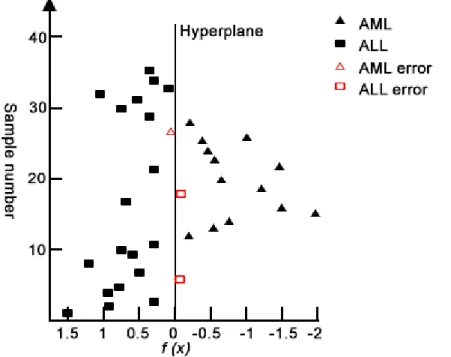
The SVM works by identifying training samples that are closest to the hyperplane and classifies an unseen sample based on this information. However, the performance of the SVM degrades when there are training samples which are very close to the hyperplane. This is illustrated in Figure 2.3.
Figure 2.3: Support Vector Machine (SVM) applied to the leukaemia dataset. Fig-ure showing the application of the Support Vector Machine approach to the leukaemia dataset. Samples indicated by hollow triangle and rectangles are closest to the hyperplane and are therefore misclassified by the Support Vector Machine [80].
k-NN works by looking at distance between an unknown test sample and known training samples and classifying the unknown sample according to the majority of its closest neighbours.
Xiaoqiao and Lin [80] used Signal-to-Noise Metric (S2N) for feature selection and used KSVM for classification.
Their results indicate that KSVM has better accuracy than eitherk-NN or SVM alone. They conclude that this may be due to the fact that KSVM gathers more support vectors during training and therefore carries more information.
Furthermore, the number of genes used in the training process has less effect on KSVM as opposed to SVM also due to the fact that KSVM carries more information. Mei et al. [52] also propose a similar hybridized k-NN-SVM approach. However, they only use an SVM for classification when k-NN classification is indecisive.
2.3
Evolutionary Algorithm/
k
-Nearest Neighbours
Algorithm
The EA/k-NN algorithm uses an EA as the search technique and k-NN algorithm as the classifier. The EA/k-NN algorithm was first reported by Siedlecki & Skalan-sky [71].
k-NN works by assigning a classification to a sample based on its closest neigh-bours.
Figure 2.4: k-Nearest Neighbours (k-NN) Technique. Figure illustrating k-Nearest Neighbours technique. Unknown type is classified as Type X using three closest neighbours.
In Figure 2.4, it is assumed that there are only two features (A & B). They are assigned to x axis and y axis. Samples are then placed in this space using their known values. A sample of unknown type can then be placed in this space by its feature values. This unknown sample can then be classified by looking at its k-NN. In Figure 2.4, unknown type can be classified as type X by looking at its 3 closest neighbours [62].
EA/k-NN algorithm was applied to Surface-Enhanced Laser Desorption and Ion-isation Time-Of-Flight (SELDI-TOF) Proteomic data by Li et al. [47]. SELDI-TOF data is usually more complicated than DNA microarray data as SELDI-TOF tends to contain more samples (hundreds of samples) and more features for each sam-ple [47].
Li et al. [47] applied EA/k-NN algorithm to find many near optimal feature sub-sets. Features were then ranked by frequency of occurrence and the most frequently occurring features were used to classify unseen data.
They concluded that EA/k-NN algorithm was able to find a subset of 10 features that was able to classify optimally between cancer and non-cancer cases in the
ovarian cancer SELDI-TOF Proteomic dataset.
Therefore, it is apparent that EA/k-NN algorithm is suited for feature selection in predictive data mining.
2.4
Two-Phase Evolutionary Algorithm/
k
-Nearest
Neighbours Algorithm
k-NN algorithm, first introduced by Fix & Hodges [18] is a fast and simple algorithm with the advantage of having good classification performance on a wide range of real world datasets [38, 64].
Siedlecki & Sklansky [38, 71], who first introduced the idea of combining an EA with k-NN algorithm, showed that a combined EA/k-NN is very efficient at finding near optimal subsets of features from a large dataset.
Jirapech-Umpai & Aitken [38, 33] showed that classification performance of se-lected subsets of features improved significantly when prior feature selection was employed. They showed this by applying EA/k-NN algorithm without prior feature selection to Golub’s leukaemia dataset [38, 22].
They used chromosomes with initial size set to 10 and a small population. This produced 68% accuracy at best on the test set, which is poor. The EA converged quickly due to the fact that the risk of getting stuck in local optima is very high with a large dataset and small chromosome size [38].
They then used RankGene software for initial feature selection. EA/k-NN algo-rithm was then applied to the 100 best genes from the initial feature selection phase. This resulted in 95% accuracy on the test set which is a very significant increase from 68%. This clearly showed that EA/k-NN performs better when applied to a reduced dataset after prior feature selection.
Stochastic search methods such as EAs return different results for different runs when applied to truly complex problems [38]. Although this could be considered an unfavourable outcome under certain circumstances, in the case of feature selection and classification, it is desirable to get different results for different runs. This is because the search method could be run multiple times and results could be pooled to produce a reduced yet diverse dataset to which further selection and classification methods could be applied.
It is also favourable as it is possible to run either the further selection & classifica-tion step or the whole process multiple times to obtain a diverse set of near optimal feature subsets. Then, it is possible to analyse frequently occurring genes within these subsets and conclude, with some confidence, that these genes are significant to the case under study [38].
Juliusdottir et al. [38], in taking this idea forward, decided to use EA/k-NN for initial feature selection as well as further selection and classification. During the first phase, the algorithm was applied to the whole dataset for feature selection. This enabled them to reduce the datasets down to smaller sizes and apply the same algorithm to these smaller datasets. Unlike filter methods, this approach has the benefit of good feature discovery without initial dimensionality reduction. They showed that the application of EA/k-NN algorithm as the pre-processing method (phase one) is capable of competitive, if not better results, compared to other more complex pre-processing methods.
It has been shown that problems with unimodal fitness landscapes where there is only one isolated global optimum with little or no information available elsewhere in the landscape are difficult to solve. Problems with such isolated peaks in the land-scape have been called needle-in-a-haystack (NIAH) problems. It has been shown that in order to make such a problem solvable by Genetic Algorithms (GAs), the fitness landscape has to be modified to decrease the isolation of the single optimum and to increase its basin of attraction [30, 7]. On the other hand, in the context of feature selection, a generally flat fitness landscape would also prevent an EA from selecting a set of genes that are relevant to the case under study.
In a feature selection and classification context, a highly sophisticated classi-fier such as an SVM may contribute to the flattening of the fitness landscape and therefore decrease the amount of useful information that is available to the EA. For example, an SVM may classify a sub-optimal feature subset with 95% accuracy. k-NN on the other hand may classify the same subset with 80% accuracy. As the classification accuracy is measured as a percentage, the maximum possible accuracy is 100%. An SVM will therefore reduce the gap between this sub-optimal feature subset and the optimal feature subset leading to a flattening of the fitness landscape. k-NN on the other hand will not flatten the landscape to the same extent as an SVM. Therefore,k-NN will guide the EA towards optimal feature subsets. Juliusdottir et al. [38] argue that, in a combined feature selection/classification context, it is highly
valuable to concentrate on classification methods that are straightforward as they will put the onus on the EA to search for subsets of genes that are strongly corre-lated to the case under study. Only then does it become possible to save money and time by letting domain experts concentrate on these genes to either find a cure for the underlying disease or come up with early diagnostic tests, which is the ultimate goal of feature selection classification on these datasets.
2.4.1
Two-Phase Evolutionary Algorithm/
k
-Nearest
Neigh-bours Algorithm Explained
Juliusdottir et al. [38] configured phase one of the two-phase EA/k-NN as described below:
• Chromosome length = 200
• Population = 30
• Generations = 500
• Selection type = Roulette wheel selection
• Elitism = Yes, elite count of 2
• Mutation rate = 0.3 (30% chance of mutating to a non-zero gene, 70% chance of removing a gene)
• Crossover = Single point crossover
• Number of neighbours (k) = 3
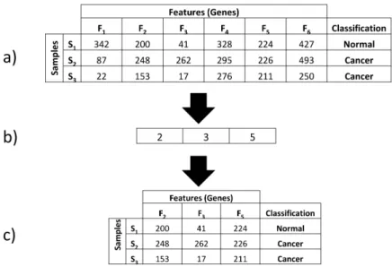
Figure 2.5 shows how a chromosome encodes a subset of features from a dataset (adapted from Juliusdottir et al. [38]).
In Figure 2.5:
a) S1, S2, S3 represents three samples from a dataset. F1 - F6 represents values for each feature in a sample.
b) An integer encoded chromosome. This chromosome is encoding features 2, 3 & 5 from the initial dataset. 2, 3 & 5 can be referred to as “selected feature subset”.
Figure 2.5: Feature selection using an integer encoded chromosome. a) An example of a dataset that has 3 samples with 6 features in each sample. b) An integer encoded chromosome that encodes 3 features. c) The dataset after it has been reduced in size using the chromosome.
c) This table shows how the dataset can be reduced using the chromosome shown in b).
Juliusdottir et al. [38] chose to represent a subset of features (i.e. a chromosome) as a variable length list of integers as shown in Figure 2.5. They argued that this encoding had the benefit of limitinga priori the size of a feature subset. They also argued that this approach had the added benefit of scalability. For large datasets (e.g. microarray data), a binary chromosome would need to contain many thousands of bits as the number of bits need to be equal to the number of attributes in the dataset.
Algorithms used in this thesis have been implemented using Java. In Java, the most efficient way of representing a binary chromosome is to represent it as an array of bytes. A byte is a primitive data type in Java that takes up exactly 1 byte of memory [23]. As the number of bits in a binary encoded chromosome needs to be equal to the number of attributes in a dataset, a binary chromosome represented in memory as a byte array will take memory equal to the number of attributes in the dataset in bytes. For example, the ovarian cancer dataset used in this thesis consists of 15154 attributes. A binary encoded chromosome can be implemented in Java using a byte array that can hold 15154 bytes. This array would take 15154 bytes of memory (excluding the overhead imposed by the Java Virtual Machine (JVM)).
An integer encoded chromosome can be implemented as an array of integers in Java. An integer takes up 4 bytes of memory in Java [23]. If an integer encoded chromosome is to represent the entire feature set (worst case scenario) of the dataset, then for the ovarian dataset, the chromosome would take up 60616 bytes (15154 x 4 bytes) of memory. However, the initial chromosome is limited to 400 features. Therefore, the initial memory imprint would be limited to 1600 bytes (400 x 4 bytes) per chromosome. One of the objectives of the algorithm is to minimise the size of the feature subset encoded by the chromosome. Therefore, most chromosomes in the population are likely to be reduced to a few features. As shown above, the shorter the chromosome, the more efficient integer encoding becomes.
There is also evidence in the literature to suggest that integer or floating point representation of a chromosome is a faster and more consistent form to run [32]. Also, an integer encoding is obvious, easy to decode and meaningful crossover and mutation operators can be applied with relative ease [12].
Fitness of a given chromosome is calculated using the Equation 2.1.
F itness= ((100−class acc)/100) + ((n/N/α) (2.1)
Where:
• class acc = mean classification performance over the three three-fold cross-validation runs
• n = size of chromosome
• N = maximum possible length for a chromosome
• α = parameter controlling trade-off between preference for accuracy and pref-erence for small subset sizes
Classification accuracy (class acc) for a given chromosome is calculated by look-ing at how many samples in the dataset that it is able to classify accurately uslook-ing k-NN algorithm.
To determine if a given chromosome (x) is capable of classifying a given sample (s1) in the dataset:
features encoded in x. E.g. for s1, calculate distance from s1 to s2, s1 to s3 and so on.
• Pick three closest neighbours to s1 from these distances.
• Determine the class of the majority of neighbours of s1. Assign this class to s1.
• Compare the known class of s1 with the assigned class. If they match, then x is capable of classifying s1 correctly using the k-NN algorithm.
The above procedure is repeated for all the data samples for a given chromosome and number of data samples that the chromosome is able to classify accurately is counted. Classification accuracy is then calculated as number of correct classifica-tions/total data samples. Once classification accuracy is known, the fitness for a given chromosome can be calculated using the Equation 2.1.
2.4.2
The Two-Phase Evolutionary Algorithm/
k
-Nearest
Neigh-bours Experimental Design
In this thesis, the two-phase EA/k-NN algorithm introduced by Juliusdottir et al. [38] is used as the baseline. In Chapter 3, a thorough investigation is carried out into the optimal way of arranging the two-phase EA/k-NN algorithm so that it performs well across a range of datasets. In Chapter 4, a weighting scheme fork-NN is investigated and a novel weighted centroid classifier is introduced in place of k-NN. Chapter 5 investigates a correlation guided mutation operator for the EA/k-NN algorithm. As the experimental design used by Juliusdottir et al. [38] is used as the basis for the following chapters, a detailed explanation of the experimental design is given in this section.
Juliusdottir et al. [38] conducted all their experiments in two phases. EA/k-NN algorithm was run on two datasets (colon [2]; prostate [72]) repeatedly during phase one. Genes that appeared in final populations were pooled together to create two large but much reduced datasets from the original datasets. EA/k-NN was then run on these reduced datasets for further selection and classification.
2.4.2.1 Phase One
This experiment was carried out on the prostate cancer dataset. The dataset had:
• 12600 features
• 52 prostate cancer samples
• 50 normal samples
The dataset was divided into training and test sets. The training set had 39 cancer and 36 normal samples. The remaining 27 samples were used as the validation set.
Set-up of the EA:
• Total number of runs = 10
• Generations = 400
• Chromosome length = 400
• Population size: 80
• Elite count: 2
• Selection: Roulette wheel selection
• Crossover: Single point crossover
• Number of neighbours fork-NN: 3
After running EA/k-NN for ten runs, the final best subsets were pooled together to form a dataset that contained 245 unique genes. This dataset was then used as the starting point for experiment 1B.
Experiment 2A
This experiment was carried out on the colon cancer dataset. The dataset had:
• 2000 features
• 40 colon cancer samples
The dataset was divided into 4 subsets of similar sizes. Three of these were used for 3-fold cross-validation (2 training, 1 testing) while the other was used as the validation set.
Set-up of the EA:
• Total number of runs = 10
• Generations = 400
• Chromosome length = 200
• Population size: 30
• Elite count: 2
• Selection: Roulette wheel selection
• Crossover: Single point crossover
• Number of neighbours fork-NN: 3
After running EA/k-NN for ten runs, the final best subsets were pooled together to form a dataset that contained 151 unique genes. This dataset was then used as the starting point for experiment 2B.
2.4.2.2 Phase Two
Experiment 1B
This experiment was run using 245 genes discovered from experiment 1A in phase one.
Set-up of the EA:
• Total number of runs = 10
• Generations = 100
• Chromosome length = 100
• Population size: 30
• Selection: Roulette wheel selection
• Crossover: Single point crossover
• Number of neighbours fork-NN: 3
The final best subsets were pooled to form a best subset of size 20. Experiment 2B
This experiment was run using 151 genes discovered from experiment 2A in phase one.
Set-up of the EA:
• Total number of runs = 8
• Generations = 100
• Chromosome length = 70
• Population size: 30
• Elite count: 2
• Selection: Roulette wheel selection
• Crossover: Single point crossover
• Number of neighbours fork-NN: 3
The final best subsets were pooled to form a best subset of size 37.
2.4.3
Results from Two-Phase Evolutionary Algorithm/
k
-Nearest Neighbours Algorithm
Using a Probabilistic Model Building Genetic Algorithm(PMBGA) with Support Vector Machine as a classifier, Topon & Iba [38, 58] managed to collect 177 different subsets. Out of these, the best subsets returned a test set accuracy of 94.12%. This subset included 24 unique genes. The smallest subset they obtained contained only 6 genes and returned 82.35% testing accuracy. They obtained an average of 84.29%
± 4.57 test set accuracy with the average number of selected genes being 17.14 ±
Singh et al. [72] used signal/noise stats together with k-NN to obtain a 16 gene subset that returned 93.12% training accuracy.
Juliusdottir et al. [38] managed to obtain 10 subsets including an average of 28 genes after applying EA/k-NN algorithm once for the whole dataset. The average test set accuracy was 87.04%. This improved to 88.88% when EA/k-NN algorithm was applied in two phases.
Although it is not possible to compare Juliusdottir et al. [38] results with others’ due to incompatibilities in experimental methodologies, Juliusdottir et al. [38] point out that it is possible to make a tentative and qualified comparison.
Singh et al. [72] used all data for training. This is not the preferred method as it is not possible to get an accurate estimate of the performance of selected subsets on unseen data if all data is used for training. The preferred method isk-fold cross-validation where the algorithm is trained on some data and other (hitherto unseen) data samples can be used to get an accurate estimate of how the selected subset would perform on unseen data. Topon & Iba [58] used a 50/50 split for training and testing. Although this is better than Singh et al. method, k-fold cross-validation is preferred over 50/50 split.
The result obtained by Juliusdottir et al. [38] on prostate cancer dataset is slightly better than Topon & Iba [58] but not as good as Singh et al. [72].
Li et al. [48] obtained 65% accuracy from a 50 gene subset using EA/k-NN approach. Liu et al. [49] achieved 91.94% classification accuracy using Leave One out Cross Validation (LOOCV).
Juliusdottir et al. [38] obtained 82.35% classification accuracy after applying EA/k-NN algorithm to the whole dataset. This improved to 94.12% when EA/k -NN method was applied in two phases. This result is better than previous reported work on this dataset.
Table 2.1 below summarises results for various approaches to feature selection and classification in prostate cancer dataset.
2.5
Multi-Objective Evolutionary Algorithms
As described in Chapter 1, it was decided that the two-phase EA/k-NN algorithm introduced by Juliusdottir et al. [38] would be used as the baseline algorithm for this thesis. As explained in Chapter 1, the objective function of the EA in the
Algorithm Classification Accuracy Length
PMBGA / SVM 94.12% 24
PMBGA / SVM 82.35% 6
Signal / noise stats with k-NN 93.12% 16
EA/k-NN 87.04% 28
Two-phase EA/k-NN 88.86% 28
Table 2.1: Summary of results for various approaches to feature selection and clas-sification in prostate cancer dataset.
two-phase EA/k-NN algorithm combines the classification error of the model with the length of the feature subset encoded by it to create a single objective value. A variable, termed α, is used in the two-phase EA/k-NN algorithm to control the trade-off between preference for classification accuracy and preference for shorter feature subsets. The effectiveness of the algorithm depends on the correct tuning of this parameter.
Therefore, the trade-off between the accuracy and the length of the model has to be calculated for each dataset the algorithm is applied to as this trade-off is critical in obtaining the best performance from the algorithm. The best way of estimating the optimal value for this parameter for a dataset is to carry out a series of experiments on the dataset. This is both resource-intensive and time-consuming.
One way of avoiding this resource-intensive and time-consuming step is to use a multi-objective EA in the two-phase EA/k-NN algorithm instead of a single ob-jective EA. The multi-obob-jective EA maximises the accuracy of the model while si-multaneously minimising the length of the selected feature subset. Therefore, with a multi-objective EA, there is no need for the parameter α.
As this problem has more than one objective (classification accuracy and the length of the feature subset) that needs to be optimised, it can be classified as a Multi-objective Optimisation Problem (MOP). A MOP can be mathematically formulated as follows [85]:
minimise F(x) = (f1(x), ..., fm(x))T
s.t. x∈Ω
(2.2)
Where Ω is the decision space and x ∈ Ω is a decision vector. F(x) consists of
The objectives in 2.2 conflict with each other and therefore multi-objective op-timisation algorithms concentrate on finding Pareto optimal solutions [76]. Pareto optimality was first introduced by Edgeworth and Pareto [85]. A solution is termed Pareto optimal if it is non-dominated with respect to all the objectives [76]. In this case, a solution can be termed Pareto optimal if there are no other solutions that are better either on classification accuracy or the length of the chromosome. All the Pareto optimal solutions, when plotted in objective space is termed as the Pareto front [76]. EAs are population based, therefore, they are able to approximate the whole Pareto front in a single run [85].
Konak et al. [1] states that the aims of a multi-objective optimisation approach should be:
1. The best-known Pareto front should be as close as possible to the true Pareto front. Ideally, the best-known Pareto set should be a subset of the Pareto optimal set.
2. Solutions in the best-known Pareto set should be uniformly distributed and diverse over the whole Pareto front in order to provide the decision-maker a true picture of trade-offs.
3. The best-known Pareto front should capture the whole spectrum of the Pareto front. This requires investigating solutions at the extreme ends of the objective function space.
These aims are readily applicable to the feature selection and classification prob-lem in large datasets as the ultimate aim is to identify feature subsets that can classify unseen samples with accuracy and robustness. If a multi-objective EA can fulfil the above aims, then the resulting Pareto front should contain feature subsets that give domain experts (e.g. oncologists) a good indication as to the promising areas for further research or putative drug targets.
Tables 2.2, 2.3 & 2.4, adapted from Konak et al. [1], lists the following multi-objective GAs:
• Vector Evaluated Genetic Algorithm (VEGA)
• Multi-Objective Genetic Algorithm (MOGA)
• Niched Pareto Genetic Algorithm (NPGA)
• Random Weighted Genetic Algorithm (RWGA)
• Pareto Envelope-based Selection Algorithm (PESA)
• Pareto Archived Evolution Strategy (PAES)
• Nondominated Sorting Genetic Algorithm (NSGA)
• Nondominated Sorting Genetic Algorithm-II (NSGA-II)
• Strength Pareto Evolutionary Algorithm (SPEA)
• Strength Pareto Evolutionary Algorithm-2 (SPEA-2)
• Rank Density-based Genetic Algorithm (RDGA)
• Dynamic Multi-Objective Evolutionary Algorithm (DMOEA)
2.6
Related Results from Literature for the Datasets
Used in This Thesis
2.6.1
Leukaemia Dataset
Bangpeng and Shao [4] introduced a novel Additive Non-parametric Margin Max-imum for Case-Based Reasoning (ANMM4CBR) method for feature selection and classification in DNA microarray datasets. They managed to obtain a best classi-fication accuracy of 97%±2.3 with 50 features on the leukaemia dataset. With 10 features, they managed to obtain an accuracy of 96.3%±2.4.
Zhu et al. [86] used a Memetic feature selection method with Filter Ranking (FR), Approximate Markov Blanket (AMB) & Affinity Propagation (AP) for fea-ture selection and classification in the leukaemia dataset. They managed to obtain 98.08% accuracy with 28.1 features.
Debnath and Kurita [15] used an evolutionary approach together with an SVM. Their approach selects new subsets of features based on the estimates of generalisa-tion error of the SVM and frequency of occurrence of the features in the evolugeneralisa-tionary approach. With this method, they managed to obtain an accuracy of 100% with 3 features on the leukaemia dataset.
Algorithm Fitness assignmen t Div ersit y mec hanism Elitism External population Adv an tages Disadv an tages VEGA [70 ] Eac h su b p op ulation is ev aluated with regards to a differen t ob jec ti v e No No No First MOGA Straigh tforw ard implemen tation T end to con v erge to the extreme of eac h ob jectiv e MOGA [19 ] P areto ranking Fitness sharing b y n ic hing No No Simple extension of single ob jectiv e GA Usually slo w con v ergence Problems related to nic he size parameter WBGA [26 ] W eigh ted a v erage of normalised ob jectiv es Nic hing Predefined w eigh ts No No Simple extension of single ob jectiv e GA Difficulties in non con v ex ob jec tiv e function space NPGA [31 ] No fitness assignmen t, tournamen t se lection Nic he coun t as tie-break er in tournamen t selection No No V ery simple selec ti on pro cess with tournamen t selection Problems related to nic he size parameter Extra parameter for tournamen t selection R W GA [55 ] W eigh ted a v erage of normalised ob jectiv es Randomly assigned w eigh ts Y es Y e s Efficien t and easy to implemen t Difficulties in non con v ex ob jec tiv e function space PESA [11 ] No fitness assignmen t Cell-based densit y Pure elitist Y es Easy to implemen t Computationally efficien t P erformance d e p ends on cell sizes Prior information needed ab out ob je ctiv e space T able 2.2: Some w ell kno wn m ulti-ob jectiv e Genetic Algo rithms adapted from Konak et al. [1 ] -part I.
Algorithm Fitness assignm e n t Div ersit y mec hanism Elitism External population Adv an tages Disadv an tages P AES [40 ] P areto domin ance is used to replace a paren t if offspring dominates Cell-based densit y as tie-break er b et w een offspring and par e n t Y es Y es Random m utation hill-clim bing str ate gy Easy to implemen t Computationally efficien t Not a p opulation based approac h P erformance dep ends on cell sizes NSGA [75 ] Ranking based on non-domination sorting Fitness sharing b y nic hing No No F ast con v ergence Problems related to nic he size parameter NSGA-I I [14 ] Ranking based on non-domination sorting Cro wding distance Y es No Single parameter (N) W ell tested Efficien t Cro wding distance w orks in ob jectiv e space only SPEA [88 ] Raking based on the external arc hiv e of non-dominated solutions Clustering to truncate external p opulation Y es Y es W ell tested No parameter for clustering Complex clustering algorithm SPEA-2 [87 ] Strength of d om in ators Densit y based on the k-th nearest neigh b or Y es Y es Impro v ed SPEA Mak e sure extreme p oin ts are preserv ed Computationally exp ensiv e fitness and densit y calculation T able 2.3: Some w ell kno wn m ulti-ob jectiv e Genetic Algo rithms adapted from Konak et al. [1 ] -part II.
Algorithm Fitness assignmen t Div ersit y mec hanism Elitism External population Adv an tages Disadv an tages RDGA [51 ] The problem reduced to bi-ob je ctiv e problem with solution rank an d densit y as ob jectiv es F orbidd e n region cell-based densit y Y es Y es Dynamic cell up date Robust with resp ec t to the n um b er of ob jectiv es More difficult to implemen t than others DMOEA [82 ] Cell-based ranking Adaptiv e c ell-based densit y Y es (implicitly) No Includes effic ie n t tec hniques to up date cellvdensities Adaptiv e ap proac hes to v set GA parameters More difficult to implemen t than others T able 2.4: Some w ell kno wn m ulti-ob jectiv e Genetic Algo rithms adapted from Konak et al. [1 ] -part II I.
2.6.2
Prostate Cancer Dataset
Mundra and Rajapakse [54] introduced an improved version of Support Vector Ma-chine - Recursive Feature Elimination (SVM-RFE) by incorporating a Minimum-Redundancy Maximum-Relevancy (MRMR) filter. With this approach, they man-aged to isolate 10 features with 98.29%±2.30 accuracy from the prostate cancer dataset.
2.6.3
Ovarian Cancer Dataset
Zhu et al. [86] also used ovarian cancer dataset with their Memetic feature selection approach. They managed to obtain 99.52% accuracy with 9 features.
2.6.4
Colon Cancer Dataset
Guyon et al. [25] proposed a feature selection method that used SVM based on Re-cursive Feature Elimination (RFE). They demonstrated that this method is