AUSTRALIAN JOURNAL OF BASIC AND APPLIED SCIENCES

(1)

AUSTRALIAN JOURNAL OF BASIC AND

APPLIED SCIENCES

ISSN:1991-8178 EISSN: 2309-8414 Journal home page: www.ajbasweb.com

Open Access Journal

Published BY AENSI Publication

This work is licensed under the Creative Commons Attribution International License (CC BY).

http://creativecommons.org/licenses/by/4.0/

To Cite This Article: Dr.D.Selvaraj and S.Satheesh kumar., Acoustic Guidance For Hearing Impaired People. Aust. J. Basic & Appl. Sci.,

10(1): 219-216, 2016

Acoustic Guidance For Hearing Impaired People

1

Dr.D.Selvaraj and 2S.Satheesh kumar

1_{Dept. of Electronics and Communication Engineering Panimalar Engineering College Chennai, India}

[email protected]

2_{Dept. of Electronics and Communication Engineering Sree Sastha Institute of Science and Technology Chennai, India}

Address For Correspondence:

Dr.D.Selvaraj, Dept. of Electronics and Communication Engineering Panimalar Engineering College Chennai, India. E-mail: [email protected]

A R T I C L E I N F O A B S T R A C T Article history:

Received 10 December 2015 Accepted 28 January 2016 Available online 10 February 2016

Keywords:

Hearing impaired, Voice recognition

This paper presents a technique for guide the people who are hearing impaired using audio classification and categorization. Here we are going to get the audio signal as the input from the environment and display the output in the form of either text or symbol. This is done in two steps namely wavelet transform which finds the features of audio signal and support vector machine which classifies and categorizes the audio signal. Even though many methods are available to classify and categorize the audio signal, the above mentioned techniques give 90% to 100% accuracy and classification errors are reduced from 8% to 3%.

INTRODUCTION

In the age of digital information, audio data has become an important part in many modern computer applications. A typical multimedia database often contains millions of audio clips, including environmental sounds, machine noise, music, animal sounds, speech sounds, and other nonspeech utterances. The need to automatically recognize to which class an audio sound belongs makes audio classification and categorization an emerging and important research area. In general, audio classification and categorization can be performed in two steps. In the first step, an audio sound is reduced to a small set of parameters using various feature extraction techniques, and in the second step, classification or categorization algorithms ranging from simple Euclidean distance methods to sophisticated statistical techniques are carried out over these parameters. The efficacy of an audio classification or categorization system depends on the ability to capture proper audio features and to accurately classify each feature set corresponding to its own class.

(2)

better than the nearest neighbor (NN), nearest center (NC), and the 5-NN classifiers, resulting in 40 classification errors when classifying 198 sounds selected from the Muscle Fish database.

Several statistical techniques, such as neural networks, hidden Markov models (HMMs), or support vector machines (SVMs), can also be applied to these parameters for audio classification and categorization. Among these techniques, SVMs, which were proposed by Vapnik (1998), have been regarded as a new learning algorithm for various applications, such as audio classification (Guo, G. and S.Z. Li, 2003; Clarkson, P. and P.J. Moreno, 1999) and pattern recognition [11]–[15]. By using SVMs instead of the NFL method, Guo and Li (2003) managed to significantly improve the previous work on classification performance. They achieved as few as 16 classification errors in classifying 198 sounds into 16 classes, or an equivalent error rate of 8.1%.

This paper adopts Guo and Li’s method and creates an improved audio classification and categorization system by incorporating additional wavelet functions and a bottom-up SVM. The improvement can be attributed to better feature extraction and SVM construction. Wavelets (Mallat, S., 1998; Burrus, C.S., 1998)] are a widely used technique that have also been applied to speech and audio feature extraction. In contrast with conventional methods using the Fourier transform, the pitch information (Chen, S.H. and J.F. Wang, 2002) and subband power (Hsieh, C.T., 2002) extracted from the wavelet domain can improve performance, as shown in various experimental results. To increase the discriminability of sounds, the overlap size between windowed frames of the proposed feature extraction algorithm is redesigned, and a normalization process is carried out after feature extraction. It is worth noting that wavelets also help the proposed method in reducing the size of the feature vector from (18+2L) to(14+2L) . In addition, this paper modifies two SVM training parameters–the upper bound C and the variance σ2 of the exponential radial basis function (ERBF)–to improve the accuracy of classification. Experimental results show that our method reduces the number of classification errors in from 16 (an error rate of 8.1%) to 6 (3.0%).

Proposed Method:

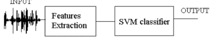
The block diagram of the proposed technique is shown in figure 1. It involves two stages to identify the audio signals

1) Feature Extraction 2) Support vector machine

Fig. 1:Block diagram of the complete process.

In first stage, the features such as sub band power, pitch frequency, bandwidth, brightness and frequency cepstral coefficient are extracted from audio signal. In second stage, support vector machine classifies or identifies the audio signals based on the training samples. The preprocessing is done before the features extraction. This is used for make the several frames. Then hamming window method pre-emphasizes the frame and calculates the power of each frame. If the power exceeds the certain threshold value, then it considers as a non silent frame. Otherwise it will consider as a silent frame and it will be neglected. Hence the features will extract from non silent frame.

Feature Extraction :

Several features are extracted from each input sound to facilitate further classification or categorization. In this paper, a (14+2L)-dimensional feature vector is proposed for audio classification and categorization. The (14+2L)-dimensional feature vector is constructed from perceptual features and frequency cepstral coefficients. Detailed preprocessing and feature extraction processes are described as follows.

A. Preprocessing:

The original audio sounds in Muscle Fish were sampled at 8000 Hz with 16-bit resolution. Each sound is divided into frames. The frame length is 256 samples (32 ms) with a 192-sample (75%) overlap between adjacent frames. Due to radiation effects of the sound from lips, high-frequency components have relatively low amplitude, which will influence the capture of the features at the high end of the spectrum. One simple solution (Chu, W. C., 2003) is to augment the energy of the high-frequency spectrum. This procedure can be implemented via a pre-emphasizing filter that is defined as

,255 1,... n for 1 n S * 0.96 n S ' n

(3)

Where sn is the nth sample of the frame s and 0 ' 0

s

=

. Then, the pre-emphasized frame is Hamming-windowed by

..,255 0,... i for i h * ' i S h i

S = =

With hi=0.54-0.46*Cos(2πi/255). The pre-processed frame will be detected as a nonsilent frame for feature extraction if the total power is large, i.e.,

2 400 2 ) h i (S 255

0 i

>

∑

=

where 400 is an experience value (Li, S.Z., 2000).

B. Feature Extraction From Nonsilent Frames:

The Fourier transform is the most popular method that maps audio signals from the time domain to the frequency domain. The wavelet transform (Mallat, S., 1998; Burrus, C.S., 1998) is another choice in many previous works. It follows from (Chen, S.H. and J.F. Wang, 2002; Hsieh, C.T., 2002) that a three-level wavelet transform, as shown in Fig. 1, gives a better performance for an audio signal with a sampling rate of 8000 Hz. Hence, this paper applies both Fourier and wavelet transforms to increase the ability to capture proper audio features.

1) Brief Introduction to the Wavelet Transform:

The wavelet transform discussed here is implemented via a filterbank structure. A fast discrete algorithm proposed by Mallat (1998) is shown in Fig.2, where h(n)and g(n) are the analysis lowpass and highpass filters. In addition, the symbol ↓2denotes the downsampling by 2.

Fig. 2: Three level wavelet transform.

Let {a3(n)}nЄz be the input to the analysis filterbank. Then, the outputs of the analysis filterbank are given by

(n) 1 i a * 2k) (n n

~ h (k) i

a =∑ − ₊ and (n 2k)*a_i ₁(n)

n ~ g (k) i

d =∑ − ₊

Where ai(k) and di(k) are called the approximation and detail coefficients of the wavelet decomposition of ai+1(n), respectively. In this paper, the calculation of the wavelet transform is implemented using the length-8 orthogonal wavelet introduced by Daubechies (Mallat, S., 1998; Burrus, C.S., 1998). Wavelet transform is nothing but a subband coding.

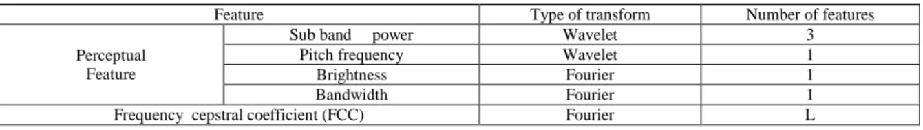
Table 1: List of extracted features.

Feature Type of transform Number of features

Perceptual Feature

Sub band power Wavelet 3

Pitch frequency Wavelet 1

Brightness Fourier 1

Bandwidth Fourier 1

Frequency cepstral coefficient (FCC) Fourier L

2) Perceptual and FCC Feature Extractions:

There are in total (6+L) features, shown in Table I, derived from wavelet coefficients and fast Fourier transform (FFT) coefficients F(u) of each nonsilent frame sih . The (6+L) features contain perceptual features and an L- order frequency cepstral coefficient (FCC). The detailed extraction process of each feature is given in the following.

a) Subband Power Pj:

(4)

approximation and detail coefficients a0(k),d0(k),and d1(k) of a given audio sound a3(k) ,respectively. The subband power pj is calculated by

(k) kz2_j j

P =∑

where zj(k) is the corresponding approximation or detail coefficients of subband.

b) Pitch Frequency fp :

A noise-robust wavelet-based pitch detection method is used to extract the pitch frequency. The first stage of the pitch-detection method is to apply the wavelet transform with aliasing compensation to decompose the input sound into three subbands. Then, this method makes use of a modified spatial correlation function, which was determined from the approximation signals obtained in the previous stage to extract the pitch frequency.

An improved wavelet-based method is developed for extracting pitch information from noisy sounds. It uses a modified spatial correlation function which is originally applied to wavelet based signal denoising to improve the performance of pitch detection in a noisy environment. The modified spatial correlation function needed in the proposed pitch detection method makes use of an aliasing compensation algorithm to eliminate the aliasing distortion that arises from the down sampling and upsampling operations of the wavelet transform. As a consequence, this allows one to further increase the accuracy of pitch detection.

c) Brightness ω_c:

The brightness is the frequency centroid of the Fourier transform and is computed as

du 2

ω

0 F(u) du/ 2

ω

0 F(u) u c

ω = ∫ ∫

d) Bandwidth B:

It is the square root of the power-weighted average of the squared difference between the spectral components and the frequency centroid, i.e.,

du 2 ω

0F(u) du/ 2 ω

0 F(u)

2 ) c ω (u

B= ∫ − ∫

e) Frequency Cepstral Coefficient (FCC): The L-order coefficients are calculated as

( )

(

log₁₀Fu

)

cos

(

n

(

u 0.5

)

π/256

)

, 2/256

n

c 255

0

u −

∑

= =

Where n=1,…., L

C. Feature Vector Formation:

The mean and the standard deviation of each of the (6+L) features are computed to result in a (12+2L) – dimensional feature vector. Furthermore, the pitch ratio (number of pitched frames/total number of frames) and the silence ratio (number of silent frames/total number of frames) are added to the above feature vector to form a (14+2L)-dimensional feature vector.

D. Normalization for Training and Testing:

An experimental audio feature set is partitioned into a training Set T and a testing set E. The detailed partition process is given in Section IV. The training set T can be defined as an nT*(14+2L) array of elements T(i,j), where nT is the number of training vectors, and the subscripts i and j denote the row and column positions, respectively.

Support Vector Machine (Svm):

Support vector machine (Pontil, M. and A. Verri, 1998; Guo, G. and S.Z. Li, 2003) have recently been proposed as popular tools for learning from experimental data. The reason is that SVMs are much more effective than other conventional nonparametric classifiers (e.g., the RBF neural networks, nearest neighbor (NN), nearest center (NC), and the -NN classifier (Schwenker, F., 2000) in terms of classification accuracy, computational time, and stability to parameter setting. They also prove to be more effective than the traditional pattern recognition approaches based on the combination of a feature selection procedure and a conventional classifier. SVMs use a known kernel function to define a hyperplane in order to separate given points into two predefined classes. An improved SVM called the soft-margin SVM can tolerate minor misclassifications. It is considered to be more suitable for classification and, therefore, is used in this paper.

A. Introduction to SVMs:

(5)

Є{-1,1}. We would like to find the equation of the hyperplane that divides S by leaving all the points of the same class on the same side, and maximizing the distance between the two classes and the hyperplane.

Definition 1. The set S is linearly separable if there exists w Є Rn such that yi(w · xi + b)>=1

for i = 1, 2, ...., N

The pair (w,b) defines a hyperplane of equation w · x + b = 0

Let w be the norm of w, then the distance di of a point xi from the hyperplane is di =(w · xi + b)/w

which combined with the above equations yields a minimum distance of 1/w. However, since our goal is to also maximize the smallest distance. The problem can be represented as

Minimize 1/2w · w

Subject to yi(w · xi + b) >=1, i = 1, 2, ...,N

B. Linearly Separable Case:

The above problem p1 can be solved by using Lagrange Multipliers. Assuming α = (α1, α 2, ..., αN)represent the N Lagrange multipliers, the problem becomes

1) b] ) x [(w, (y w

2

1 N i i

i + −

−

=

∑

−1 j 2

α

L

At the saddle point dl/db = dl/dw = 0. Thus creating a new problem called the dual problem Minimize 1/2_αTDα +∑αi

Subject to ∑yiαi = 0, for α>= 0

where both sums are for i = 1, 2, ...., N, and D is an NxN matric such that Dij = YiYjXi·Xj.

Fig. 3: Linear separation.

The only αs in the above equation are ones that satisfy the constraint (1) with the equality sign. Therefore most of the αs are null, hence making the vector w a linear combination of relatively small percentage of points. These points are called support vectors as they represent only the points in S that are needed to determine the optimal separating hyperplane. The problem of classifying a new data point x is now to check the sign of w*x + b.

C. Linearly Non-Separable Case:

If the points in set S cannot be separated into two classes on different sides of a line, OSH cannot be found as in the linear case. Therefore, N nonnegative variables ξ = (ξ1, ξ2, ..., ξn) are introduced that allow a small fraction of points in one class to be classifies on the other side. Equation (1) now becomes

[

i

]

i,

i

ξ 1 b x w,

y + ≥ −

for i = 1, 2, ...., N

The generalized problem then becomes Minimize

∑

+ ,

2 2 1

i C

w ξ

subject

[

]

i, i

i

ξ 1 b x w,

y + ≥ −

(6)

Fig. 4: Margin and slack variable for a classification.

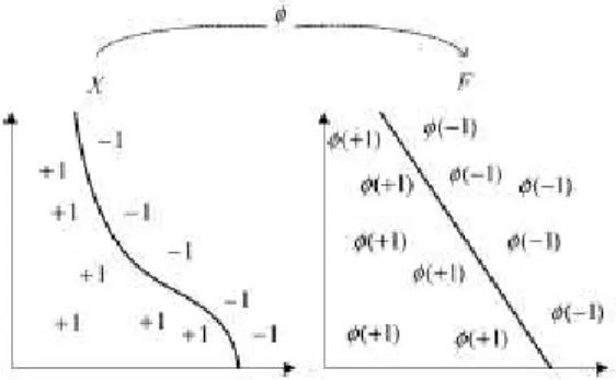
Fig. 5: Feature map can simplify the classification task.

The purpose of C is to act as a regularization parameter. It leads to a more robust solution in the sense that for small C the OSH maximizes the minimum distance 1/w, and for large C the OSH minimizes the number of misclassified points.

Minimize 1/2_αTDα +∑αi

Subject to ∑yiαi = 0, for 0<=αi<=c And i = 1, 2, ...., N

There are three common kernel functions for the nonlinear feature mapping, shown in Figure. 5

1)ERBF

    

   ₋

−

= ₂

' '

2 exp ) , (

σ

x x x

x k

2) Gaussian function:

 

 

 



 ₋

−

= 2

2 / '

2 exp ) , (

σ x x x

x k

where parameter σ2 is the variance of the Gaussian function, and

3) polynomial function

:_k₍_x_,_x'₎=

(

_x_,_x' +₁

)

d

where parameter d is the degree of the polynomial. Many classification problems are always separable in feature space and are able to obtain better accuracy by using the Gaussian kernel function than the linear and polynomial kernel functions (Melgani, F. and L. Bruzzone, 2004; Clarkson, P. and P.J. Moreno, 1999; Ganapathiraju, A., 2004; Schwenker, F., 2000). Recently, Guo and Li (2003) proposed the ERBF function as the kernel function and produced vastly improved results.

D. Multicase Classification in SVMs:

(7)

ii. One-against-all: Classify between each class and all other remaining classes.

iii. Top-down binary tree: An initial group contains all classes. A recursive process is done to separate and reduce a larger candidate group of classes into a smaller one until the test pattern is assigned to a final class. iv. Bottom-up binary tree: A recursive comparison process is performed between pairs of classes. The class

with a shorter distance from the test pattern is retained for further comparison until the test pattern is assigned to a final class.

Experimental results:

We performed different sets of experiments with different audio signals. We applied the support vector machine algorithm. It classifies the audio signals with less misclassification errors. The result will be displayed in the form of image and text. The training audio signals are taken for train the machine according to the features which is extracted from training samples. While testing, the features of test signal is calculated as shown in figure 6. If test signal is clap, then features are 0.0112 0.0870 1.2642 25.3731 0.0064 0.0808 0.4673 0.4376 9.7954. If the test signal is voice of Selvaraj, then the features are 0.5528 0.7325 1.5020 23.5751 1.0372 1.0077 1.2725 0.7011 12.6078

(a) Audio Signal

(b) Voice Signal

Fig. 6: Test Signal.

Conclusion:

In this paper, we are going to guide the people who are hearing impaired. Audio signal is classified or identified using support vector machine algorithm. Even thought many method such as nearest feature line, nearest neighbor, neural networks, hidden Markov models (HMMs) are available, SVM is faster than other techniques. Experimental results show that our method reduces the number of classification errors from 16 (an error rate of 8.1%) to 6 (3.0%). The categorization accuracy of a given audio sound can achieve 97.0% and 100%..

REFERENCES

Wood, E., T. Blum, D. Keislar, J. Wheaton, 1996. “Content-based classification, search and retrieval of audio,” IEEE Multimedia, 3(3): 27–36.

Li, S.Z., 2000. “Content-based audio classification and retrieval using the nearest feature line method,” IEEE Trans. Speech Audio Process., 8(5): 619–625.

Zhang, T. and C.C.J. Kuo, 2001. “Audio content analysis for online audiovisual data segmentation and classification,” IEEE Trans. Speech Audio Process., 9(4): 441–457.

Lu, L., H.J. Zhang, H. Jiang, 2002. “Content analysis for audio classification and segmentation,” IEEE Trans. Speech Audio Process., 10(7): 504–516.

Guo, G. and S.Z. Li, 2003. “Content-based audio classification and retrieval by support vector machines,” IEEE Trans. Neural Networks, 14(1): 209–215.

Melgani, F. and L. Bruzzone, 2004. “Classification of hyperspectral remote sensing images with support vector machines,” IEEE Trans. Geosci. Remote Sens., 42(8): 1778–1790.

Clarkson, P. and P.J. Moreno, 1999. “On the use of support vector machines for phonetic classification,” in Proc. IEEE Int. Conf. Acoustics, Speech, Signal Process., 2: 585–588.

Vapnik, V.N., 1998. Statistical Learning Theory. New York: Wiley.

(8)

Ding, P., Z. Chen, Y. Liu, B. Xu, 2002. “Asymmetrical support vector machines and applications in speech processing,” in Proc. IEEE Int. Conf. Acoustics, Speech, Signal Process., 1: I-73–I-76.

Ganapathiraju, A., J.E. Hamaker, J. Picone, 2004. “Applications of support vector machines to speech recognition,” IEEE Trans. Signal Process., 52(8): 2348–2355.

Schwenker, F., 2000. “Hierarchical support vector machines for multi-class pattern recognition,” in Proc. IEEE Fourth Int. Conf. Knowledge-Based Intelligent Eng. Syst. Allied Technologies, 2: 561–565.

Luo, T., K. Kramer, D.B. Goldgof, L.O. Hall, S. Samson, A. Remsen, T. Hopkins, 2004. “Recognizing plankton images from the shadow image particle profiling evaluation recorder,” IEEE Trans. Syst., Man Cybern.—B: Cybern., 34(4): 1753–1762.

Fenglei, H. and W. Bingxi, 2001. “Text-independent speaker recognition using support vector machine,” in Proc. Int. Conf. Info-Tech Info-Net, 3: 402–407.

Pontil, M. and A. Verri, 1998. “Support vector machines for 3-D object recognition,” IEEE Trans. Pattern Anal. Machine Intell., 20(6): 637–646.

Mallat, S., 1998. A Wavelet Tour of Signal Processing. New York: Academic.

Burrus, C.S., R.A. Gopinath, H. Guo, 1998. Introduction to Wavelets and Wavelet Transforms. Englewood Cliffs, NJ: Prentice-Hall.

Chen, S.H. and J.F. Wang, 2002. “Noise-robust pitch detection method using wavelet transform with aliasing compensation,” Proc. Inst. Elect. Eng. Vision, Image Signal Process., 149(6): 327–334.

Hsieh, C.T., E. Lai, Y.C. Wang, 2002. “Robust speech features based on wavelet transform with application to speaker identification,” Proc. Inst. Elect. Eng. Vision, Image Signal Process., 149(2): 108–114.