HAL Id: lirmm-01083542
https://hal-lirmm.ccsd.cnrs.fr/lirmm-01083542
Submitted on 17 Nov 2014
HAL
is a multi-disciplinary open access
archive for the deposit and dissemination of
sci-entific research documents, whether they are
pub-lished or not. The documents may come from
teaching and research institutions in France or
abroad, or from public or private research centers.
L’archive ouverte pluridisciplinaire
HAL
, est
destinée au dépôt et à la diffusion de documents
scientifiques de niveau recherche, publiés ou non,
émanant des établissements d’enseignement et de
recherche français ou étrangers, des laboratoires
publics ou privés.
Graph Minors and Parameterized Algorithm Design
Dimitrios M. Thilikos
To cite this version:
Dimitrios M. Thilikos. Graph Minors and Parameterized Algorithm Design. The Multivariate
Al-gorithmic Revolution and Beyond, LNCS (7370), pp.228-256, 2012, Essays Dedicated to Michael R.
Fellows on the Occasion of His 60th Birthday - Part II, 978-3-642-30890-1.
�10.1007/978-3-642-30891-8_13�. �lirmm-01083542�
Graph Minors and Parameterized
Algorithm Design
?Dimitrios M. Thilikos??
Department of Mathematics, National and Kapodistrian University of Athens, Panepistimioupolis, GR-15784, Athens, Greece
Abstract The Graph Minors Theory, developed by Robertson and Sey-mour, has been one of the most influential mathematical theories in pa-rameterized algorithm design. We present some of the basic algorithmic techniques and methods that emerged from this theory. We discuss its direct meta-algorithmic consequences, we present the algorithmic appli-cations of core theorems such as the grid-exclusion theorem, and we give a brief description of the irrelevant vertex technique.
Keywords:graph minors, parameterized algorithms, treewidth, bidimensional-ity, irrelevant vertex technique, linkages.
1
Introduction
Graph Minors Theory (GMT) was developed by Robertson and Seymour in a series of 23 papers, between 1984 and 2009. Among them, the second paper of the series was published in the Journal of Algorithms while all the rest were pub-lished in the Journal of Combinatorial Theory Series B. The main theoretical achievement of this project was the proof of Wagner’s conjecture, now known as theRobertson & Seymour Theorem, stating that graphs are well-quasi-ordered under the minor containment relation. Besides its purely mathematical impor-tance, GMT induced a series of powerful algorithmic results and techniques that had a deep influence on theoretical computer science. More particularly, GMT has been one of the most powerful “mathematical engines” in the theory and design of parameterized algorithms. In particular, a considerable part of the ba-sic techniques in parameterized algorithm design is directly or indirectly linked to results from GMT. Moreover, GMT offered the theoretical base for the un-derstanding and resolution of some of the most prominent graph-algorithmic problems in parameterized complexity. In what follows, we give a brief presen-tation of the main results and techniques in this area.
?
This research has been co-financed by the European Union (European Social Fund – ESF) and Greek national funds through the Operational Program “Education and Lifelong Learning” of the National Strategic Reference Framework (NSRF) -Research Funding Program: “Thalis. Investing in knowledge society through the European Social Fund”.
??
Our presentation is organized as follows. In Section 2 we give the definitions of some basic combinatorial and algorithmic concepts. In Section 3.1 we present the main algorithmic consequences of the GMT, mainly from the parameterized complexity viewpoint. Section 4 is devoted to the celebrated grid-exclusion theo-rem and its applications to bidimensionality theory. Finally, Section 5, attempts a short presentation of the irrelevant vertex technique and its applications.
2
Basic definitions
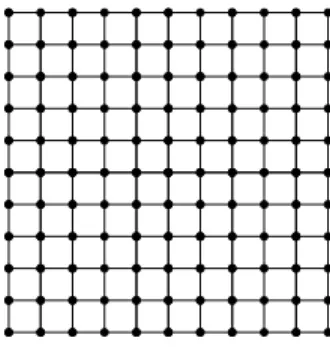
All graphs we consider are finite, undirected and simple, i.e., they do not have multiple edges or loops. Given a graph G we denote by V(G) and E(G) its vertex and edge set respectively. Thesize(reps.magnetite) of a graph Gis the number of its vertices (reps. edges) and is denoted by n(G) (reps. m(G)), i.e., n(G) = |V(G)| (m(G) = |E(G)|). We denote by G\v the graph obtained by removingv (along with its incident edges) fromG. Theneighborhoodof a vertex v ∈V(G), denoted by NG(v), is the set of edges in G that are adjacent to v. The degree of a vertex v ∈ V(G) is the cardinality of its neighborhood in G. We denote by Kr the complete graph on r vertices and by Kr,q the complete bipartite graph with r vertices in its one part and q in the other. Finally, we denote byGk the (k×k)-grid, i.e., the Cartesian product of two paths of length k−1 (see Figure 1).
Our presentation is organized as follows. In Section 2 we give the definitions of some basic combinatorial and algorithmic concepts. In Section 3.1 we present the main algorithmic consequences of the GMT, mainly from the parameterized complexity viewpoint. Section 4 is devoted to the celebrated grid-exclusion theo-rem and its applications to bidimensionality theory. Finally, Section 5, attempts a short presentation of the irrelevant vertex technique and its applications.
2
Basic definitions
All graphs we consider are finite, undirected and simple, i.e., they do not have multiple edges or loops. Given a graph G we denote by V(G) and E(G) its vertex and edge set respectively. Thesize (reps.magnetite) of a graphGis the number of its vertices (reps. edges) and is denoted by n(G) (reps. m(G)), i.e., n(G) = |V(G)| (m(G) = |E(G)|). We denote by G\v the graph obtained by removingv(along with its incident edges) fromG. Theneighborhoodof a vertex v 2 V(G), denoted byNG(v), is the set of edges inG that are adjacent to v. The degreeof a vertex v 2 V(G) is the cardinality of its neighborhood in G. We denote by Kr the complete graph on r vertices and by Kr,q the complete bipartite graph with r vertices in its one part and q in the other. Finally, we denote byGk the (k⇥k)-grid, i.e., the Cartesian product of two paths of length k 1 (see Figure 1).
Figure 1.The (11,11)-gridG11.
2.1 Relations on graphs and obstructions
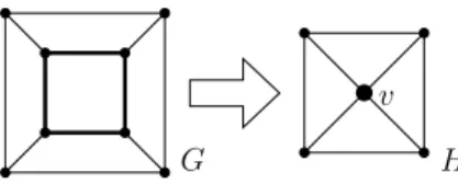
We say that a graphH is asubgraphof a graphGifH can be obtained byGby removing edges or vertices. The contraction of an edgee={x, y}fromGis the removal fromGof all edges incident toxoryand the insertion of a new vertex ve that is made adjacent to all the vertices of (NG(x)\ {y})[(NG(y)\ {x}). Given two graphs H and G, we say that H is a contractionof G, denoted by
Figure 1.The (11,11)-gridG11.
2.1 Relations on graphs and obstructions
We say that a graphH is asubgraphof a graphGifH can be obtained byGby removing edges or vertices. The contraction of an edgee={x, y}from Gis the removal fromGof all edges incident toxor yand the insertion of a new vertex ve that is made adjacent to all the vertices of (NG(x)\ {y})∪(NG(y)\ {x}).
Given two graphs H and G, we say that H is a contraction of G, denoted by H ≤c G, if H can be obtained from G by a (possibly empty) series of edge contractions.
H c G, if H can be obtained from G by a (possibly empty) series of edge
contractions.
G H
v
Figure 2. The graphH is the result of the contractions of the bold edges inG
to the vertexv.
H is aminorofGifHis a contraction of some subgraph ofG. A graphH is atopological minorofG(denoted byHtG) ifGcontains as a subgraph some
subdivision ofH(asubdivisionof a graphH is any graph obtained by replacing some of its edges by paths between the same endpoints). Given a partial ordering relationon graphs, we say that a graph class G isclosed under if for every
G2 G, HG implies thatH 2 G. LetG be a graph class that is closed under the minor relation. An -anti-chain is a set of graphs that are pairwise non-comparable with respect to. For example the set of graphsA={K2,r |r 2}
is a c-antichain but not anm-antichain or at-antichain.
We define the -obstruction setof a graph class G, denoted byobs(G), as the set of all -minimal graphs thatdo notbelong to G. Clearly, by definition, the-obstruction set of a graph class is an-anti-chain. Obstruction sets can be seen as alternative characterizations of graph classes and, in many cases, reveal a good deal from their structural characteristics. For example, it easy to verify that
obsm(T) = obst(T) = {K3}, obsm(O) =obst(O) = {K4, K2,3}, where
T and O are the classes of all acyclic and all outerplanar graphs respectively, and obsc(O⇤) = {K4, K2,3, K
+
2,3} where O⇤ are the connected outerplanar
graphs and K2+,3 is the graph obtained from K5 by removing a triangle. The
most classic theorems on obstruction characterization of graph classes are the Kuratowski-Pontryagin’s theorem [87] and Wagner’s theorem [121], stating that
obsm(P) = {K5, K3,3} and obst(P) = {K5, K3,3} respectively, where P is
the class of all planar graphs.
2.2 Parameterized problems and algorithms
The idea of problem parameterization is to treat algorithmic problems as param-eterized entities and to evaluate the complexity of the corresponding algorithms by considering the way parameters appear in their running times. As here we deal with problems on graphs, we adapt the classic definitions of parameterized complexity to the case where problem inputs represent graphs.
Formally, a parameterized problem on graphsis a subset⇧ of⌃⇤⇥N, where ⌃ is some alphabet and, in each (I, k) 2 ⌃⇤ ⇥N, I encodes a combinatorial
Figure 2.The graph H is the result of the contractions of the bold edges inG to the vertexv.
H is aminorofGifH is a contraction of some subgraph ofG. A graphH is atopological minorofG(denoted byH ≤tG) ifGcontains as a subgraph some subdivision ofH (asubdivisionof a graphH is any graph obtained by replacing some of its edges by paths between the same endpoints). Given a partial ordering relation≤on graphs, we say that a graph classG isclosed under≤if for every G∈ G,H ≤Gimplies that H ∈ G. LetG be a graph class that is closed under the minor relation. An ≤-anti-chain is a set of graphs that are pairwise non-comparable with respect to≤. For example the set of graphsA={K2,r |r≥2} is a ≤c-antichain but not an ≤m-antichain or a≤t-antichain.
We define the≤-obstruction set of a graph classG, denoted byobs≤(G), as the set of all≤-minimal graphs thatdo notbelong toG. Clearly, by definition, the≤-obstruction set of a graph class is an≤-anti-chain. Obstruction sets can be seen as alternative characterizations of graph classes and, in many cases, reveal a good deal from their structural characteristics. For example, it easy to verify that obs≤m(T) = obs≤t(T) = {K3}, obs≤m(O) = obs≤t(O) = {K4, K2,3}, where
T and O are the classes of all acyclic and all outerplanar graphs respectively, and obs≤c(O∗) = {K4, K2,3, K
+
2,3} where O∗ are the connected outerplanar graphs and K2+,3 is the graph obtained from K5 by removing a triangle. The most classic theorems on obstruction characterization of graph classes are the Kuratowski-Pontryagin’s theorem [87] and Wagner’s theorem [121], stating that obs≤m(P) = {K5, K3,3} and obs≤t(P) = {K5, K3,3} respectively, where P is
the class of all planar graphs.
2.2 Parameterized problems and algorithms
The idea of problem parameterization is to treat algorithmic problems as param-eterized entities and to evaluate the complexity of the corresponding algorithms by considering the way parameters appear in their running times. As here we deal with problems on graphs, we adapt the classic definitions of parameterized complexity to the case where problem inputs represent graphs.
Formally, aparameterized problem on graphsis a subsetΠ ofΣ∗×N, where Σ is some alphabet and, in each (I, k) ∈ Σ∗×N, I encodes a combinatorial structure related to one, or more, graphs. For this, we agree thatn(resp.m) is the maximum size (resp. magnitude) of the graphs encoded in I and we insist that |(I, k)| = O(m). We call I the main part of the input and we say that k is the parameter of the problem. Two instances (I, k),(I0, k0) ∈ Σ∗×N are equivalent with respect to Π if (I, k)∈Π ⇐⇒ (I0, k0)∈Π.
We say thatΠ isfixed parameter tractableif there exists a function1f :N
→
Nand an algorithm deciding whether (I, k)∈Π in O(f(k)·nc) steps, wherec is a constant not depending on the parameter k of the problem. We call such an algorithmFPT-algorithmor, to express concretely the choice of f andc, we say thatΠ ∈O(f(k)·nc)-FPT. A parameterized problem on graphs belongs to the parameterized class FPT if it can be solved by an FPT-algorithm. In fact, not all parameterized problems belong to the classFPT. There is a hierarchy of parameterized complexity classes, namely
FPT⊆W[1]⊆W[2]⊆W[3]⊆. . .⊆W[SAT]⊆W[P]⊆XP,
and appropriate parameter-preservingreductions such that, when a problem is hard for some of them (other than FPT), it is not expected to have an FPT -algorithm (all inclusions in this hierarchy are believed to be strict). See the monographs [39, 44, 97] for more details on parameterized complexity.
Time bounds for parameterized algorithms have two parts. The termf(k) is called parameter dependenceand, is typically a super-polynomial function. On the other hand, the term nc is a polynomial function and we call itpolynomial part. In most of the problems that we examine here,Iwill encode a simple graph. To simplify notation, we frequently write “Ok(nc)” instead of “f(k)·(nc)” for somerecursive functionf :N→N” and, in this case, we refer to the functionf hidden in theOk notation as theparameter dependence.
3
Algorithmic consequences of the GMT
3.1 Well-Quasi-Ordering
The main combinatorial result of the GMT fits in the more general framework of the theory of Well-Quasi-Orderings, first developed by Graham Higman2under the name “finite basis property” [65]. Given a set X and a partial ordering ≤ on X we say that X is well-quasi-ordered under ≤ if none of its subsets is an infinite≤-antichain.
Theorem 1 (Robertson & Seymour Theorem [110]).The set of all graphs is well-quasi-ordered under minors.
1
Notice that in the definition ofFPTf is not necessarily a recursive function.
2 As mentioned in [86], the same theory was also developed in some unpublished
manuscript of Erd˝os and Rado, while its first hints can be traced back to B. H. Neu-mann [96]
In other words, Theorem 1 says that If G is an infinite set of graphs then there exist two graphs H, G ∈ G such that H is a minor of G. The proof of theorem 1 was concluded in paper XX of the Graph Minors Series. Before its proof, the statement of Theorem 1 was known as Wagner’s conjecture. However, as mentioned by Diestel in [32], Wagner said that he had never made such a conjecture. A similar conjecture, on the well-quasi-ordering of trees under the topological minor relation was made by V´azsonyi and was proved in 1960 inde-pendently3 by Joseph Kruskal and S. Tarkowski [91]. Interesting results on the meta-mathematics of Kruskal’s tree theorem as well as Roberson & Seymour’s theorem can be found in [55] and [54] respectively.
Consider the following parameterized problem: H-Minor Checking
Instance: Two graphsGandH.
Parameter:k=|V(H)|.
Question: IsH a minor ofG?
The main algorithmic contribution of the GMT is the following result.
Theorem 2 (Robertson and Seymour [108]). One can construct an algo-rithm that, given an-vertex graphGand a k-vertex graphH, checks whetherH is a minor of a graphGinOk(n3)steps. In other words,H-Minor Checking∈ Ok(n3)-FPT.
Actually, Robertson and Seymour in [108] describe anOk(n3)-step algorithm that solves a generalization of theH-Minor Checkingand another celebrated problem, namely thek-Disjoint Pathsproblem. In Section 5, we give a rough description of the main ingredients of the algorithm in Theorem 2 especially for thek-Disjoint Pathsproblem. Recently, this running time was improved to a quadratic one for thek-Disjoint Pathsproblem in [74].
The good news about Theorem 2 is that it is constructive (contrary to The-orem 1) and there is a recursive function hidden in the Ok notation. The bad news is that, according to the algorithm in [108] and the proof of its correctness in [111] and [107], the values of this function areimmense4, even for small values ofk. David Johnson mentioned in [67]:
“for any instanceG= (V, E)that one could fit into the known universe, one would easily prefer|V|70to even constant time, if that constant had
to be one of Robertson and Seymour’s”.
Moreover, in [67], David Johnson estimates that just one constant in the param-eter dependence of Theorem 2 is roughly
2↑222
2↑2↑Θ(r)
3
A shorter and quite elegant proof of V´azsonyi’s conjecture was given by Nash-Williams in 1963 [95].
4
Perhaps the word “immense” is somehow moderate here. Instead, Fellows and Langston used the expression “mind-boggling” in [43].
where 2↑r denotes a tower 222. . .
involvingr2’s. Clearly, such type of constants may create reasonable doubts to computer scientists on whether such an algo-rithm may be considered to be an “algoalgo-rithm” of some practical meaning. In fact, to investigate until which point these constants can be improved is an open and challenging problem in parameterized complexity and algorithms (see e.g. [3]).
3.2 Minor-closed graph parameters
Aparameter on graphs(ora graph parameter) is any function that maps graphs to integers and with the property that it is invariant under graph isomorphism. Let≤be a relation on graphs. We say that a graph parameterpisclosed under
≤(or, simply, ≤-closed) if for every two graph H and G, H ≤Gimplies that p(H) ≤ p(G). We define the ≤-obstruction family of p as the parameterized graph class
O≤p,k=obs≤({G|p(G)≤k}). Consider the following parameterized meta-problem.
k-Parameter Checking forp
Instance: a graphGand an integerk≥0.
Parameter:k
Question: p(G)≤k?
Theorems 1 and 2 together have the following dramatic consequence. Theorem 3. For every parameterpthat is closed under minors there exists an algorithm that solves the problem k-Parameter Checking for pinf(k)·n3 steps for some functionf.
Proof. Recall that, by definition, no two graphs in O≤m
p,k can be comparable graphs under the minor relation. It follows, from Theorem 1, that O≤m
p,k is a finite set. Let g(k) =|O≤m
p,k|. Aspis closed under minors, it holds that p(G)≤k ⇐⇒ ∀H ∈ O≤m
p,k H 6≤mG.
Therefore, to check whether p(G) ≤ k it is enough to apply g(k) times the Ok(n3) step algorithm of Theorem 2 and check whether some member of Op≤,km is contained as a minor inG.
Theorem 3 had a great impact in parameterized complexity as it implied a massive classification of problems in the class FPT. In that sense, Theorem 3 is an algorithmic meta-theorem because it provides a generic condition (minor-closedness) for a parameterized problem that automatically implies the existence of an FPT-algorithm for it. Unfortunately, the proof of Theorem 1 does not provide any general “meta-algorithm” to compute the set O≤m
p,k and, that way, construct the claimed algorithm for eachp. In fact, due to the meta-mathematics
of Theorem 1 [54], such an meta-algorithm does not exist. As observed in [43], there is no algorithm that, given a Turing machine accepting precisely the graphs of a minor-closed graph class F, outputs obs≤m(F) (see also [119]). However,
Theorem 3 gave important (mathematical) energy to Parameterized Algorithms as it acted as an “encouraging factor”. The knowledge that an algorithm exists for a specific problem, induces the challenge to construct one and, in a sense, provides the courage to try to accomplish such a task.
In order to cope with the inherent non-constructivity of Theorem 3 one may study specific parameters where the computation of the setO≤m
p,k (or, at least, of some upper bound to the function g(k)) in the proof of Theorem 3 is possible. However, this is not an easy task, even for simple parameters. According to [34], if the problem of checking whether p(G) ≤ k is NP-complete, then |O≤m
p,k| is a super-polynomial function of k, unless the polynomial hierarchy collapses to ΣP
3. Characterizations of p(G) ≤ k (yielding better lower bounds for |Op≤,km|) have been provided for several parameters [10, 20, 40, 58, 84, 98, 99, 115, 117, 118]. However, to our knowledge, there is not yet a natural parameterpfor which a complete characterization ofO≤m
p,k is known. A more promising strategy towards detecting constructive fragments of Theorem 3, is to detect parameters – or families of parameters – whereO≤m
p,k is recursive. For this one may either prove upper bounds for|O≤m
p,k|, as done in [57] for the case of branchwidth5, or provide partial characterizations of O≤m
p,k, as done in [2, 19, 21, 89, 94], that permit its recursive computation.
At this point, we should mention that all theorems of this section have their counterparts in another partial relation on graphs, the one of immersion. The lift of two incident edges is the operation of removing two edges e1 = {x, y} and e2 ={x, z} (incident to a common vertex x) and adding the edge {y, z}. We say that a graph H can be immersed in a graphG, denoted byH ≤im G, ifH can be obtained from a subgraph of Gby a (possibly empty) sequence of edge lifts. According to the last paper of the Graph Minor series [112], graphs are well-quasi-ordered under immersions, i.e., Theorem 1 holds also if we replace minors by immersions. Therefore, in order to prove a counterpart of Theorem 3 for the case of immersion-closed parameters, we need an algorithm that given an n-vertex graphGand ak-vertex graphH, checks whereH ≤imGinOk·(n(G))3 steps. Recently, a construction of such an algorithm was given in [61]. This makes it possible to derive the following meta-algorthmic result.
Theorem 4. If p is a parameter that is closed under immersions, then there exists an algorithm that solves the problem k-Parameter Checking forpin f0(k)·n3 steps for some functionf0.
In fact, the main result of [61] proves theFPT membership of topological minor testing, i.e., given two graphsH andG, check whether H ≤tG(the
pa-5
Branchwidth was introduced in the paper X of the Graph Minor Series [106] and, from that point and then, was used as an alternative for treewidth (defined formally in Section 4). Treewidth and branchwidth can be seen as twin parameters, as the one is a constant factor approximation of the other.
rameter is the size of H). This means that there is a counterpart of Theorem 2 for the topological minor relation as well. This might create some hope that Theorem 3 holds for topological minors as well. Unfortunately, this requires an analogue of the combinatorial Theorem 1 which does not exist as it is possible to construct an infinite class of graphs that are pairwise non-comparable with respect to the topological minor relation: just take all cycles with their edges duplicated. An other argument for the non-existence of analogues of Theorems 1 and 3 for topological minors is given by theTopological Bandwidth prob-lem asking whether the topological bandwidth of a graph is at most k. The topological bandwidth of a graphGis denoted by tbw(G) and is defined as
tbw(G) = min{k| ∃q≥1 :G≤tPqk} (Pk
q is obtained by a pathPq of lengthqif we make adjacent any two vertices of distance ≤kin Pq). It is easy to observe that tbw is closed under topological minors. In [42] it is mentioned thatTopological BandwidthisW[t]-hard for allt ≥1 – the proof is a modification of the proof for the case of Bandwidth
in [15]. This implies that, under reasonable assumptions in parameterized com-plexity theory, the anti-chain corresponding to the≤t-obstruction familyO≤tbwt ,k is infinite for an infinite set of values ofk.
4
Grid-exclusion and bidimensionality
4.1 Treewidth
Treewidth has been one of the main contributions of GMT to algorithmic graph theory. While, as a concept, its indices can be traced back to the work of Gavril in [56], its formal birth as a graph parameter occurred in the second paper of the Graph Minors series [104]. Currently, there are at least six equivalent definitions of tree-width. We present the original one from [104].
A tree decomposition of a graph G is a pair (X, T) where T is a tree and
X ={Xi|i∈V(T)} is a collection of subsets ofV(G) such that: 1. Si∈V(T)Xi=V(G);
2. for each edge{x, y} ∈E(G),{x, y} ⊆Xi for somei∈V(T), and
3. for eachx∈V(G) the set{i|x∈Xi}induces a connected subtree ofT. Thewidthof a tree decomposition ({Xi|i∈V(T)}, T) is maxi∈V(T){|Xi| −1}. Thetreewidth of a graphG, denoted by tw(G), is the minimum width over all tree decompositions ofG.
If, in the above definitions, we restrict the treeT to be a path then we define the notions ofpath decomposition andpathwidth. We writepw(G) to denote the pathwidth of a graph G. Pathwidth was defined earlier than treewidth in the first paper is the Graph Minors Series [102].
Treewidth can intuitively be seen as a measure of the topological resemblance of a graph to a tree or, alternatively, as a measure of the “global connectivity”
of a graph. Similarly, pathwidth can be seen as a measure of the topological resemblance of a graph to a path.
Counting Monadic Second Order Logic (CMSOL) is a logic on graphs6where the domain is the set of vertices and edges, there are predicates for vertex-vertex adjacency and edge-vertex incidence, there is quantification over edges, vertices, edge sets and vertex sets, and there is a predicate Cardr,p(S) which expresses whether the size of a setS isrmodulop.
The importance of treewidth for algorithmic graph theory is illustrated by the celebrated Courcelle’s theorem stating that ifΠkis a parameterized property of graphs expressible by a CMSOL formulaφk, then there is an algorithm that, given as input a graphG, can check whetherGsatisfies propertyΠk(i.e., whether G∈Πk) inO|φk|+tw(G)(n) steps. Moreover, there exists a meta-algorithm that,
given φk, outputs such an algorithm. A proof of Courcelle’s theorem can be found in [39, Chapter 6.5] and [44, Chapter 10] and similar results appeared by Arnborg, Lagergren, and Seese in [8] and Borie, Parker, and Tovey in [17]. An alternative game-theoretic proof has appeared recently in [81, 82].
Courcelle’s theorem had a deep influence in parameterized algorithms as it automatically yieldsFPT-algoriths for a wide family of problems, provided that the treewidth of their instances is bounded by a function of the parameterk. The natural challenge is whether and when a parameterized problem can be reduced to its bounded treewidth variant. For this, an important step is to detect what kind of combinatorial structures are contained in a graph with big treewidth. The most prominent structure of this type is the grid Gk. Let gm(G) be the maximumkfor whichGcontainsGk as a minor. A valuable theoretical tool in this direction was given by the following result of the GMT.
Theorem 5 ( [105]). There exists a recursive function f : N → N such that tw(G)≤f(gm(G)).
While the above result appeared in the fifth paper of the series, a prelimi-nary variant of it, where Gis planar, appeared earlier in [103]. As every graph containingGk as a minor has treewidth at leastk, Theorem 5 implies thattw and gm are parametrically equivalent: a bound to the one of them implies a bound to the other. The initial estimation of the parameter dependence in The-orem 5 was huge. However, a better one appeared in [113] where it was proven thattw(G) = 202·(gm(G))5
. An alternative, and relatively simpler, proof of The-orem 5 was given in [33]. To see the use of TheThe-orem 5 in parameterized algorithm design, consider a parameterpthat satisfies the following properties:
i. pis closed under taking of minors.
ii. there exists a recursive functiont:N→Nsuch that p(Gt(k))> kfor every non-negative integerk.
iii. One can construct an algorithm that, given a tree-decomposition of G of width at mostqand an integerk, checks whetherp(G)≤kinl(k, q)·nO(1) steps for some recursive functionl:N×N→N.
6
We should stress that CMSOL is not only a logic on graphs but also on more general combinatorial objects calledstrucures.
Clearly, the first two conditions are easy to check for most instantiations of p. Moreover, the third one follows directly from Courcelle’s theorem if for each k, Πk = {G | p(G) ≤ k} is expressible by a CMSOL formula φk. There are many examples of such parameters. Typical examples are the vertex cover of a graph, i.e., the minimum number of vertices that meets all vertices ofGand the feedback vertex set of a graph, i.e., the minimum number of vertices meeting all cycles ofG. A direct consequence of Theorem 5 is the following (constructive) special case of Theorem 3:
Lemma 1. Letpbe a parameter satisfying conditionsi–iiiabove for sometand l. Then it is possible to construct an algorithm that, given as input a graph G and an integerk, checks whetherp(G)≤kin(2O(f(t(k))+l(k,4
·f(t(k))))·nO(1) steps wheref is the function in Theorem 5.
Proof. The algorithm in Lemma 1 works as follows: First of all, it uses anFPT -approximation algorithm for treewidth, i.e., an algorithm that given a graphG and an integer q, either outputs a tree decomposition of G of width at most α·q or reports that tw(G) > q in z(q)·nβ steps. Various algorithms of this type have been proposed in [7, 14, 88, 100, 108] for different trade-offs betweenz, α, and β. Among them, we pick the one form [7] where z(q) = 24.38·q, α= 4, and β = 2. We run this algorithm for Gand q = f(t(k)). If it outputs a tree decomposition of width≤4·f(t(k)) then we use the algorithm of Property iii and solve the problem inl(k,4·f(t(k)))·nO(1)steps. If the algorithm reports that the treewidth ofGis more thanf(t(k)), then from Theorem 5,GcontainsGt(k) as a minor. In such a case, the algorithm directly outputs a negative answer as, from Propertiesiandii,p(G)≥p(Gt(k))> k.
The idea of the above proof is also known as theWin/win approach: we either have an answer to the problems directly because the treewidth is big enough or we solve the problems use dynamic programming on a tree-decomposition of bounded width.
Clearly, the running time of the algorithm in Lemma 1 depends on the func-tions f, t, and l. In what follows, we comment on the current bounds on each one of them.
l: As we have already mentioned, the (constructive) existence ofl, follows from Courcelle’s theorem for the wide family of problems that are expressible in CMSOL. However, the bounds onl, derived from the proof, are huge and this may dismiss any hope for a good parameter dependence (see [53]). However, for many problems it is possible to directly apply dynamic programing on the tree decomposition and derive moderate bounds on l such as l(k, q) = 2O(q2)·kO(1), orl(k, q) = 2O(qlogq)·kO(1)or, even better,l(k, q) = 2O(q)·kO(1). Clearly, time bounds of the third type are more attractive. For this reason, we say that a parameter p is single exponentially solvable with respect to treewidth if there exists an algorithm that, given Gand k, checks whether p(G)≤k in 2O(tw(G))
·nO(1) steps. There is a quite extended bibliography on how to do fast dynamic programming on graphs of bounded treewidth;
as a sample of this, we just mention [5, 6,9,11,13,16,22,35,35–37,37,38,114, 120, 120].
t: Bounds are much better for the functiont. For most natural graph param-eters, it holds that t(k) = O(k) while for some of them, includingtw and pw, it holds thatt(k) =Θ(k). However, there is a wide family of parameters where t(k) = O(√k). This intuitively says that a certificate for the value of such a parameter spreads “bidimensionally” inside a (k×k)-grid. For in-stance any vertex cover ofGkshould have size at leastk·bk2c=Ω(k2) as the vertices of such a set should cover edges all over the “area” of the grid. Sim-ilarly, a feedback vertex set ofGk should have size at least (bk2c)2 =Ω(k2) as the vertices of such a set should cover all (bk
2c)2 members of a packing of “squares” inGk.
If such a parameter is also closed under taking of minors then we call it minor bidimensional.
f: To improve the function f, i.e., the parameter dependence in Theorem 5, is an important challenge as, even for the parameters with most moderate instantiations oflandt,k-Parameter Checking forpcould be only clas-sified in 22kO(1)
·nO(1)-FPT. Robertson, Seymour, and Thomas conjectured in [113] thatf can be a polynomial function. This would directly imply that k-Parameter Checking for p belongs to 2kO(1) ·nO(1)-FPT for a wide family of parameters (see [30] for more discussions and conjectures on this issue).
Another interesting problem is to lower bound the contribution off in The-orem 5. As mentioned by Robertson, Seymour, and Thomas in [113] there are graphs excludingGk as a minor that have treewidth Ω(k2·logk). To see this, one may use the result in [23] (see also [41, 122]) to construct an O(1)-regular Ramanujan graphGonnvertices that has girthΩ(logn). One can easily verify thatgm(G) =O(log√nn). The claimed bound follows because Ramanujan graphs are expanders and thustw(G) =Ω(n). It is a challenging question whether any bound better than this one can be proven.
Towards achieving a polynomial dependance between treewidth and the size of an excluded grid, Reed and Wood defined in [101] the notion of a grid-like-minor. Agrid-like-minor of orderk in a graphGis a set of paths inG whose intersection graph is bipartite and contains aKk as a minor. Clearly, the rows and columns of the (k×k)-grid are a grid-like-minor of orderk+ 1. In [101] it is proved that every graph with treewidthΩ(k4√logk) contains a grid-like minor of order k. Meta-algorithmic implications of the results in [101], analogous to those of Theorem 1, can be found in [85].
4.2 Bidimensionality
Theorem 5 has several refinements that are important for improving the pa-rameter dependence of the algorithm in Lemma 1. The first variant of Theo-rem 5 for special graph classes appeared in [113] (proved for the twin param-eter of branchwidth) from which it follows that if G is a planar graph, then
tw(G)≤6·gm(G). Actually, with some more careful application of the results of [113] it can also be proven thattw(G)≤5·gm(G), which can be improved further to tw(G) ≤ 9
2 ·gm(G) using the results of [62]. An analogous upper bound holds also for graphs embedded in surfaces. From the results in [27], it follows that tw(G)≤6·(eg(G) + 1)·gm(G) where eg(G) is the Euler genus of G. Also in [30], it was proven that if G is a K3,r-minor free graph, then tw(G)≤204r
·gm(G). At this point, the natural question is whether this lin-ear dependence holds for every non-trivial minor-closed graph class. This was resolved in [29], where the following theorem has been proved.
Theorem 6. Let r be a positive integer. If G is a Kr-minor free graph, then tw(G) =Or(gm(G)).
The proof of Theorem 6 is heavily based on GMT. More specifically, it depends on the Structure Theorem of the GMT [109] which implies immense bounds for the parameter dependence of the bound in Theorem 6. The improve-ment of the parameter dependance of Theorem 6 is an interesting problem and this might be possible without making use of the structural results of [109].
As mentioned in the previous Section, a parameterpisminor-bidimensional if it is closed under taking of minors and for every non-negative integerkit holds that p(Gd√
ke) =Ω(k). A major consequence of Lemma 1, Theorem 6, and the discussion above is the following meta-algorithmic result.
Theorem 7. LetH be anr-vertex graph and letpbe a graph parameter that is minor-bidimensional and single exponentially solvable with respect to treewidth. Thenk-Parameter Checking forprestricted toH-minor free graphs belongs (constructively) to2Or(
√ k)
·nO(1)-FPT, i.e., one can construct a sub-exponential FPT-algorithm that solves it.
Notice that the above result is, in a sense, optimal, as, due to the complexity bounds in [18], a 2O(√k)
·nO(1)-step parameterized algorithm is the best we may expect for several bidimensional parameters, even on planar graphs. The meta-algorithmic machinery that we employed above in order to prove Theorem 7 is known asBidimensionality Theoryand was introduced for the first time in [27], while some preliminary ideas had already appeared in [4, 52].
Theorem 7 concerns only minor-closed parameters. A typical parameter that does not fit in the framework of minor-bidimensionality is the dominating set number, denoted byds(G) and defined as the minimum size of adominating set in G, i.e., a setS of vertices such that every vertex not inS has some neighbor in S.
The dominating set number is not minor-closed as it may increase by remov-ing edges. However this is not the case when we do only contractions. To develop the contraction counterpart of bidimensionality, one has to find a counterpart of Theorem 6 for contractions, i.e., to detect what types of graphs appear as contractions in graphs with big treewidth. This line of research was developed in [26, 31] and concluded in [46]. Before we present the the results in [46], we need first some definitions.
LetΓk (k≥2) be the graph obtained from the (k×k)-grid by triangulating internal faces of the (k×k)-grid such that all internal vertices become of degree 6, all non-corner external vertices are of degree 4, and then one corner of degree two is joined by edges with all vertices of the external face (the corners are the vertices that in the underlying grid have degree two). Graph Γ6 is shown in Fig. 3. Let also Πk be the graph obtained from Γk by adding a new vertex
Let
k(
k
2) be the graph obtained from the (
k
⇥
k
)-grid by triangulating
internal faces of the (
k
⇥
k
)-grid such that all internal vertices become of degree
6, all non-corner external vertices are of degree 4, and then one corner of degree
two is joined by edges with all vertices of the external face (the
corners
are
the vertices that in the underlying grid have degree two). Graph
6is shown
in Fig. 3. Let also
⇧
kbe the graph obtained from
kby adding a new vertex
Figure 3.
The graph
6.
adjacent to all vertices of
k.
A consequence of the results in [46] is the following.
Theorem 8.
There exists a function
↵
:
N
!
N
such that every connected
graph of treewidth at least
↵
(
k
)
contains some of the graphs in
{
K
k,
k, ⇧
k}
as
a contraction.
Theorem 8 has several refinements. One of them is the following counterpart
of Theorem 6.
Theorem 9.
There exists a function
:
N
!
N
such that every connected
K
r-minor-free graph of treewidth at least
(
r
)
·
k
2contains either
kor
⇧
kas a
contraction.
Notice that in the above theorem, the quadratic dependence (on
k
) is optimal.
Indeed, let
Z
k2be the graph obtained by adding to
G
k2a new vertex adjacent
to all the
k
2vertices with both coordinates in the underlying grid divisible by
k
.
Then
Z
k2excludes
K
6,
G
k+2, and
⇧
k+2as contractions and is of treewidth at
least
k
2. This means that, in order to have a “linear counterpart” of Theorem 6,
we should restrict further the graphs that we exclude. An
apex graph
is a graph
that can become planar by the removal of one vertex. It appears that the linear
dependence in the bound of Theorem 6 is also possible for contractions when
we consider graphs excluding some apex graph as a minor. For this, we define
tgm
(
G
) as the maximum
k
for which
G
contains
kas a contraction.
Figure 3.The graphΓ6.adjacent to all vertices ofΓk.
A consequence of the results in [46] is the following.
Theorem 8. There exists a function α : N → N such that every connected graph of treewidth at least α(k)contains some of the graphs in {Kk, Γk, Πk} as a contraction.
Theorem 8 has several refinements. One of them is the following counterpart of Theorem 6.
Theorem 9. There exists a functionβ:N→Nsuch that every connectedK r-minor-free graph of treewidth at least β(r)·k2 contains either Γ
k or Πk as a contraction.
Notice that in the above theorem, the quadratic dependence (onk) is optimal. Indeed, letZk2 be the graph obtained by adding toGk2 a new vertex adjacent
to all thek2vertices with both coordinates in the underlying grid divisible byk. Then Zk2 excludes K6, Gk+2, andΠk+2 as contractions and is of treewidth at
leastk2. This means that, in order to have a “linear counterpart” of Theorem 6, we should restrict further the graphs that we exclude. Anapex graphis a graph that can become planar by the removal of one vertex. It appears that the linear dependence in the bound of Theorem 6 is also possible for contractions when
we consider graphs excluding some apex graph as a minor. For this, we define tgm(G) as the maximumkfor whichGcontainsΓk as a contraction.
Theorem 10. Let H be an apex graph with r vertices. If Gis a connected H -minor-free graph, then tw(G) =Or(tgm(G)).
We say that a parameterpiscontraction bidimensionalif it is closed under taking of contractions and if p(Γd√
ke) = Ω(k) for every non-negative integer k. Using now Theorem 10 one can derive the following contraction counterpart of Theorem 7.
Theorem 11. Let H be an r-vertex apex graph and let p be graph parameter that is contraction-bidimensional and single exponentially solvable with respect to treewidth. Then k-Parameter Checking for prestricted toH-minor free graphs belongs (constructively) to2Or(
√ k)
·nO(1)-FPT, i.e., one can construct a sub-exponential FPT-algorithm that solves it.
The algorithmic consequence of Theorems 6 and 10 are not restricted in the design of sub-exponential parameterized algorithms (i.e., Theorems 7 and 11). Bidimensionality theory had meta-algorthmic applications in the automatic deriva-tion of linear-time kernels for wide families of parameterized problems [12, 51]. Apart from its applications to parameterized complexity, Bidimensionality The-ory was also used for the automated design of Fast Polynomial Time Approxi-mation Schemes (FPTAS) in [28] and [48].
Proving extensions of Theorems 7 and 11 for wider families of graph classes (possibly with worse – but still moderate – time bounds) is a open challenge in parameterized algorithm design. For this, one may either need to find extensions of Theorems 6 and 10 for graph classes that are wider than H-minor free and apex-minor free graphs respectively (see [50] for an important step in this direc-tion) or to invent alternative notions of grid-like structures whose presence in a graph is still able to certify a big enough value for the parameterp(see [85,101] and the end of Subsection 4.1).
5
The irrelevant vertex technique
One of the most powerful tools in parameterized algorithm design is the irrel-evant vertex technique, introduced in [108] in order to derive (among others)
FPT-algorithms for theH-Minor Checking(Theorem 2) and thek-Disjoint PathsProblem. The formal definition of the latter is the following.
k-Disjoint Paths
Instance: A graphGand a sequence of pairs
terminalsT = (s1, t1), . . . ,(sk, tk)∈(V(G)×V(G))k.
Parameter:k.
Question: Are therekpairwise vertex disjoint paths
P1, . . . , Pk inGsuch that for everyi∈ {1, . . . , k}, Pi has endpointssi andti?
We stress that, in [108], bothH-Minor Checkingandk-Disjoint Paths
where treated simultaneously and the methodology that we present below is sim-ilar for both of them. In this section we give an outline of theOk(n3) algorithm in [108] for the k-Disjoint Paths problem and we present some of the most important combinatorial results that supported the proof of its correctness. 5.1 The general framework
Given an instance (G, T, k) of the k-Disjoint Paths problem, we say that a vertex v ∈ V(G) is an irrelevant vertex of G if (G, T, k) and (G\v, T, k) are equivalent instances of the problem.
The general scheme of the algorithm in [108] is the following: Irrelevant Vertex for the classGk
Input:An instance (G, T, k) ofk-Disjoint Paths
Output:A (reduced) equivalent instance ofk-Disjoint Paths
1.whileG6∈ Gk,
2. findan irrelevant vertexv inG 3. set G←G\v
4.output(G, T, k)
Clearly, each variant of the above scheme depends on the parameterized class
Gk and creates an equivalent instance that belongs toGk. The algorithm in [108] applies the above scheme in twophases: the first phase considers
Gk ={G|Gis aKh(k)-minor free graph}
for some recursive functionhand produces equivalent instances where the input graph does not contain a “big clique” as a minor. The second phase assumes that the input graph excludes such a clique and considers
Gk ={G|Gis aGg(k)-minor free graph},
for some recursive functiong:N→N. This produces an equivalent instance that, from Theorem 5, has treewidth bounded byOk(1) and, in this case, the problem can by solved in Ok(n) steps, using dynamic programming or, alternatively, by just using Courcelle’s theorem.
It now remains to explain how Step 2 of the above scheme (i.e., finding an irrelevant vertex) is implemented in each of these two phases.
We omit the description of the first phase. Instead, we restrict ourselves to the second phase, as it encompasses the most combinatorially rich part of [108]. We just mention that the function his determined from the results in [108] on the correctness of the first phase. The functiongwill be defined in the course of the description of the second phase below.
Assume now that we have an instance (G, T, k) ofk-Disjoint Pathswhere G excludes a clique Kh(k) as a minor but, however, it still contains a the grid Gg(k)as a minor which means thattw(G)≥g(k). A big part of [108] is devoted
to the characterization of such graphs, i.e., of H-minor free graphs with “big” treewidth. In particular, a major achievement of [108] was to show the Weak Structure Theorem of GMT, stating that such graphs contain some portion that is, in a sense, “almost flat”. At this point we postpone the description of the irrelevant vertex technique to Subsection 5.3 in order to give the precise statement of this theorem.
5.2 The weak structure graph minors theorem
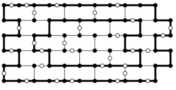
Walls. Awall of heightk,k≥1, is the graph obtained from a ((k+1)×(2·k +2))-grid with vertices (x, y),x∈ {1, . . . ,2·k+ 2},y∈ {1, . . . , k+ 1}, by the removal of the “vertical” edges {(x, y),(x, y+ 1)} for oddx+y, and then the removal of all vertices of degree 1. We denote such a wall by Wk. The corners of the wall Wk are the verticesc1 = (1,1), c2= (2·k+ 1,0), c3 = (2·k+ 1 + (k+ 1 mod 2), k+ 1) andc4= (1 + (k+ 1 mod 2), k+ 1). We letC={c1, c2, c3, c4}. A subdivided wallW of heightkis a graph obtained fromWk by replacing some of its edges by paths without common internal vertices. We call the resulting graph W asubdivisionofWk. TheperimeterPof a subdivided wall is the cycle defined by its boundary. Thelayers of a subdivided wallW of heightk are recursively defined as follows. The first layer of W is its perimeter. For i = 2,· · · ,bk
2c, the i-th layer ofW is the (i−1)-th layer of the subwall W0 obtained from W by removing from W its perimeter and all occurring vertices of degree 1 (see Figure 4).
to the characterization of such graphs, i.e., of H-minor free graphs with “big” treewidth. In particular, a major achievement of [108] was to show the Weak Structure Theorem of GMT, stating that such graphs contain some portion that is, in a sense, “almost flat”. At this point we postpone the description of the irrelevant vertex technique to Subsection 5.3 in order to give the precise statement of this theorem.
5.2 The weak structure graph minors theorem
Walls. Awall of heightk,k 1, is the graph obtained from a ((k+1)⇥(2·k +2))-grid with vertices (x, y),x2 {1, . . . ,2·k+ 2},y2 {1, . . . , k+ 1}, by the removal of the “vertical” edges{(x, y),(x, y+ 1)} for odd x+y, and then the removal of all vertices of degree 1. We denote such a wall by Wk. The corners of the wallWk are the vertices c1 = (1,1), c2 = (2·k+ 1,0),c3= (2·k+ 1 + (k+ 1 mod 2), k+ 1) andc4= (1 + (k+ 1 mod 2), k+ 1). We letC ={c1, c2, c3, c4}. A subdivided wallW of heightkis a graph obtained fromWk by replacing some of its edges by paths without common internal vertices. We call the resulting graph W asubdivisionofWk. TheperimeterP of a subdivided wall is the cycle defined by its boundary. Thelayersof a subdivided wall W of heightk are recursively defined as follows. The first layer of W is its perimeter. For i = 2,· · ·,bk
2c, the i-th layer ofW is the (i 1)-th layer of the subwallW0 obtained fromW by removing from W its perimeter and all occurring vertices of degree 1 (see Figure 4).
Figure 4.A subdivided wall of height 5 and its two first layers. The first layer is its boundary.
Compasses and rural divisions. LetW be a subdivided wall inG. LetK0be the connected component of G\P that containsW \P. The compassK ofW in Gis the graph G[V(K0)[V(P)]. Observe that W is a subgraph of K and K is connected. We say that a path of K is perimetric if its endpoints lie in the Figure 4.A subdivided wall of height 5 and its two first layers. The first layer is its boundary.
Compasses and rural divisions. LetW be a subdivided wall inG. LetK0be the connected component of G\P that containsW \P. Thecompass K of W in G is the graph G[V(K0)∪V(P)]. Observe thatW is a subgraph of K and K is connected. We say that a path of K is perimetric if its endpoints lie in the perimeterP ofW. LetP1 andP2 be two perimetric paths ofK with endpoints
a1, b1anda2, b2respectively. We say thatP1 andP2 crossinKif (a1, a2, b1, b2) is the cyclic ordering of their endpoints inP. We say that a wall isflat in Gif K does not contain any pair of crossing and vertex-disjoint perimetric paths.
IfJ is a subgraph ofK, we denote by ∂KJ the set of all verticesv ∈V(J) such that either v ∈C or v is incident with an edge ofK that is not in J. A rural divisionDof the compassKis a collection (D1, D2, . . . , Dm) of subgraphs ofK with the following properties:
1. {E(D1), E(D2), . . . , E(Dm)} is a partition of non-empty subsets ofE(K), 2. for i, j ∈[m], if i 6=j then ∂KDi 6=∂KDj and V(Di)∩V(Dj) =∂KDi∩
∂KDj,
3. for each i∈[m] and allx, y∈∂KDi there exists a (x, y)-path inDi with no internal vertex in∂KDi,
4. for eachi∈[m],|∂KDi| ≤3, and 5. the hypergraph HK = (
[ i∈[m]
∂KDi,{∂KDi|i∈[m]}) can be embedded in a closed disk∆such thatc1, c2, c3andc4appear in this order on the boundary of∆and for each hyperedgeeofHK there exist|e|mutually vertex-disjoint paths betweeneandC inK.
We call the elements ofDflaps. A flapD∈ DisinternalifV(D)∩V(P) =∅. We can now state one of the main results in [108], known as theWeak Structure Graph Minors theorem.
Theorem 12 ( [108]). There exist recursive functions g1 : N×N → N and g2 : N→N, such that for every two graphsH andG and every q∈N, one of the following holds:
1. H is a minor ofG,
2. tw(G)≤g1(q, r), wherer=|V(H)|
3. ∃X ⊆V(G) with|X| ≤g2(r) such that G\X contains as a subgraph a flat subdivided wallW whereW has height qand the compass of W has a rural divisionD such that each internal flap ofDhas treewidth at most g1(r, q). While the statement of Theorem 12 above is somehow complicated, the in-tuition behind it is simpler. It says that when a graph excludes some “small” graph H as a minor and has “big enough” treewidth, it is enough to remove a “few” vertices from it, i.e., the vertices inX, and take a graphG\X where it is possible to detect a subdivided wallW that is situated in a “flat” territory inside its perimeter P. The part of Gthat is inside P is the compass K ofW which can be seen as the union of a collection of graphs (flaps) that are tree-like (have bounded treewidth) and are “planted” in that territory. Theorem 12 was used also in [2, 24] with the name “the Trinity Lemma”. However, a more depictive alternative nomenclature might be the “Sunny Forest Lemma”, in the sense that the compassK is a forest, whose trees are the flaps, andX is the sun throwing its rays at it!
In [59], an optimized version of the above result was proved whereg1(r, q) = Or(q) and g2(r) is equal to the apex number of H, i.e., the minimum number
of vertices that, when removed from H, leave a planar graph. This improved version can easily yield both Theorems 6 and 10. In case H is an apex graph, i.e., it can become planar with the removal of a single vertex, the result in [59] implies thatX =∅ which gives an analogue of Theorem 12 for apex minor-free graphs. As, in this case, the “sun”X does not exist, we are tempted to call this “apex”-variant of Theorem 12 the “Dark Forest Lemma”.
5.3 Irrelevant vertices and linkages
We now go back to the task of detecting an irrelevant vertex in a graphGthat excludesKh(k) and has treewidth bigger thang(k). Recall that, at this point,h has already been determined so that the previous phase of the algorithm runs correctly. In what follows, we setg(k) =g1(f0(k)·f1(λ(k)), h(k)) whereg1is the function in Theorem 12, f0(k) =d√2ke+ 1, andf1 and λ will be determined later.
According to [108], it is possible, inOk(n2) steps, to detect inGa setX and a subdivided wallW of heightq=f0(k)·f1(λ(k)) ofG\X where|X| ≤g2(h(k)), as indicated in Theorem 12. For simplicity, we restrict our presentation to the case whereXis an empty set, i.e.,|X|= 0. Even if the ideas for the more general case are of the same flavor, they are quite more complicated and we prefer to omit them here.
Using a counting argument based on the definition of f0, it is easy to see that W contains a subdivided wall W0 of height q0 =f1(λ(k)) whose compass K0 avoids all terminals of the pairs inT.
The next step of the algorithm in [108] is based on the claim that if we take q0 to be “big enough”, then any vertex vmid of the inner layerLin ofW0 is an irrelevant vertex and therefore it can be safely removed from G. While such a vertex is easy to detect, to proof that it is indeed irrelevant – for some suitable choice ofq0– is not easy. We just mention that papers XXI [111] and XXII [107] of the Graph Minor series where devoted to it. Below, we present only some basic notions and ideas used in this proof. For this, we first need the definition of a k-linkage, introduced in [111].
A k-linkage in a graph G is a set of k pairwise disjoint paths of it. The endpointsof a linkageLare the endpoints of the paths inL. ThepatternofLis defined as
π(L) ={{s, t} | Lcontains a path from stot}
Twok-linkages areequivalentif they have the same pattern.
W.l.o.g. we assume that all terminals involved inT are distinct. This implies that every solution to the k-Disjoint Paths problem is a k-linkage, whose pattern is determined by the pairs inT. To prove the irrelevance of the vertex vmid, it is enough to show that any linkage L whose paths meet Lin can be replaced with an equivalent one that avoids it. To obtain an idea of how paths in Lmay reside insideK0, we need to make some observations.
LetRbe the linkage defined by the connected components of (SL∈LL)∩K0, i.e., the subpaths of the paths inLthat are “cropped” by the compassK0(notice
Figure 5. A subdivided wall W0 and the way a 13-linkage L is traversing its compassK0. The only vertices that are depicted are the endpoints of the paths inL(white vertices). The only edges that are depicted are those of the paths in
L and the edges ofW0. The grey area contains the vertices and the edges of the
graphGthat do not belong to K0.
LetRbe the linkage defined by the connected components of (SL2LL)\K0, i.e., the subpaths of the paths inLthat are “cropped” by the compassK0(notice
that all paths inRare perimetric). By the flatness ofW0, it is not possible that
two paths inRcross inK0. Moreover, by the definition of the the rural division
D0 of K0, each layer of W0, di↵erent than the inner one, is a separator of G.
Therefore, if a path in Rmeets layers Li and Lj fori j, then it should also
meet layerLµfor everyµ2 {i, . . . , j}. These observations argue that, intuitively,
paths inRcrossK0 as ifK0 where a graph embedded in a disk bounded byP –
see Figure 5 for a visualization of this. One may now claim that the infrastructure of a “big enough” subdivided wall W0 should provide enough space inside K0
so that the paths ofL could be rerouted to an equivalent linkage that does not enter very deeply inside K0. To formalize this claim Robertson and Seymour
defined the notion of a vital linkage in [111].
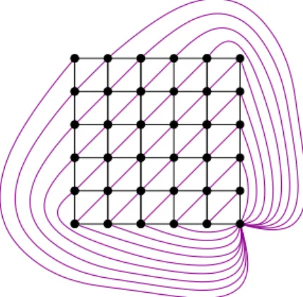
A linkageL in a graphGis calledvitalif its vertices meet all the vertices of
G and if there is no other linkage inG that is equivalent toL. An example of a vital k-linkage in a graph is depicted in Figure 6. Clearly, if a solution of the
k-Disjoint Paths Problem corresponds to a vital linkage, then no irrelevant vertex can be detected. The main result of [111] asserts that this possible “lack of flexibility” of linkages vanishes when graphs have big enough treewidth.
Theorem 13. There exists a recursive function : N ! N such that every graph with a vital k-linkage has treewidth at most (k).
Figure 5. A subdivided wall W0 and the way a 13-linkage L is traversing its compassK0. The only vertices that are depicted are the endpoints of the paths inL(white vertices). The only edges that are depicted are those of the paths in
Land the edges ofW0. The grey area contains the vertices and the edges of the graph Gthat do not belong toK0.
that all paths inRare perimetric). By the flatness ofW0, it is not possible that two paths inRcross inK0. Moreover, by the definition of the the rural division
D0 of K0, each layer of W0, different than the inner one, is a separator of G. Therefore, if a path in Rmeets layers Li and Lj fori ≤j, then it should also meet layerLµfor everyµ∈ {i, . . . , j}. These observations argue that, intuitively, paths inRcrossK0 as ifK0where a graph embedded in a disk bounded byP – see Figure 5 for a visualization of this. One may now claim that the infrastructure of a “big enough” subdivided wall W0 should provide enough space inside K0 so that the paths ofLcould be rerouted to an equivalent linkage that does not enter very deeply inside K0. To formalize this claim Robertson and Seymour defined the notion of a vital linkage in [111].
A linkageLin a graphGis calledvitalif its vertices meet all the vertices of G and if there is no other linkage inGthat is equivalent to L. An example of a vital k-linkage in a graph is depicted in Figure 6. Clearly, if a solution of the k-Disjoint Paths Problem corresponds to a vital linkage, then no irrelevant vertex can be detected. The main result of [111] asserts that this possible “lack of flexibility” of linkages vanishes when graphs have big enough treewidth. Theorem 13. There exists a recursive function λ : N → N such that every graph with a vitalk-linkage has treewidth at mostλ(k).
Actually, it was also proved in [111] that treewidth can be replaced by path-width in Theorem 13. As the proof of 13 uses the Structure Theorem of the
GMT [109], the upper bound forλthat follows from [111] is immense. However it was proved in [3] that in the case of planar graphs it holds thatλ(k) = 2O(k). Moreover, this bound is, in a sense, tight: as argued in [3], for eachkit is possible to construct a planar graph that contains a vital k-linkage and has treewidth 2Ω(k) (the 5-linkage in the graph of Figure 6 already gives the flavor of such a construction).
Actually, it was also proved in [111] that treewidth can be replaced by path-width in Theorem 13. As the proof of 13 uses the Structure Theorem of the GMT [109], the upper bound for that follows from [111] is immense. However it was proved in [3] that in the case of planar graphs it holds that (k) = 2O(k).
Moreover, this bound is, in a sense, tight: as argued in [3], for eachkit is possible to construct a planar graph that contains a vital k-linkage and has treewidth 2⌦(k) (the 5-linkage in the graph of Figure 6 already gives the flavor of such a
construction).
Figure 6.A graph of treewidth 17 and a vital 5-linkage in it.
Let nowG0be the subgraph ofGdefined by the union of the paths inL, and
the compass K0 of W0. At this point, a naive idea might be to directly apply Theorem 13 and set q0 = (k) so that the linkage Lof G0, corresponding to a
solution of thek-Disjoint Pathsproblem, cannot be vital. However, from this alone, we cannot expect nothing better than avoiding some vertices that will not necessarily be the vertices in Lin. Therefore, a non-vital linkage alone does not
provide the flexibility we need in order to reroute inG0the paths ofLin a way
that Lin is avoided.
Curiously, it appears that the importance of non-vital linkages is rather qual-itative than quantqual-itative. Based on their “elementary” flexibility, it is possible to prove that none of the paths in R “bounces” much. In particular,L can be chosen in a way that if a path inRmeets some layerLi in two di↵erent vertices x and y, then its subpath between x and y will not meet any layer Lj where
|i j| f1( (k)), for some recursive function f1. This directly implies that
paths in Rdo not go deeper than layerLf1( (k))and thus they avoidLin when q0 = f1( (k)). That way, it is possible to prove what we need: if the height of W0isf1( (k)), then another linkage, equivalent toLexists inG0(and therefore
inG as well) that avoidsLin.
We should stress that even if the above sketch might be “convincing” for a good-tempered reader, it is far from being a formal proof. In the more realistic case where X is non-empty, a more complicated criterion for the choice of the
Figure 6.A graph of treewidth 17 and a vital 5-linkage in it.
Let nowG0be the subgraph ofGdefined by the union of the paths inL, and the compass K0 of W0. At this point, a naive idea might be to directly apply Theorem 13 and setq0 =λ(k) so that the linkage L of G0, corresponding to a solution of thek-Disjoint Pathsproblem, cannot be vital. However, from this alone, we cannot expect nothing better than avoiding some vertices that will not necessarily be the vertices inLin. Therefore, a non-vital linkage alone does not provide the flexibility we need in order to reroute inG0 the paths of Lin a way that Linis avoided.
Curiously, it appears that the importance of non-vital linkages is rather qual-itative than quantqual-itative. Based on their “elementary” flexibility, it is possible to prove that none of the paths in R“bounces” much. In particular, L can be chosen in a way that if a path inRmeets some layerLiin two different vertices x and y, then its subpath between xand y will not meet any layer Lj where
|i−j| ≥ f1(λ(k)), for some recursive function f1. This directly implies that paths in Rdo not go deeper than layerLf1(λ(k)) and thus they avoid Lin when
q0 =f1(λ(k)). That way, it is possible to prove what we need: if the height of W0 isf1(λ(k)), then another linkage, equivalent toLexists inG0 (and therefore in Gas well) that avoidsLin.
We should stress that even if the above sketch might be “convincing” for a good-tempered reader, it is far from being a formal proof. In the more realistic case whereX is non-empty, a more complicated criterion for the choice of the
subdivided wall W0 should be devised and a bigger lower bound for the height ofW0 is necessary so that it contains an irrelevant vertex. In fact, this requires bigger lower bounds for bothf0 andf1. The whole proof is quite technical and has been the main purpose of [107].
According to the above discussion, the second phase of the algorithm runs in Ok(n3) steps and outputs a graph of treewidth at most g(k). As proved in [116], thek-Disjoint Pathsproblem can be solved by af2(k)·nstep dynamic programming algorithm wheref2(k) = 2O(klogk)(see [1,90] for results related to this problem). As the parameter dependence of the running time of this last step is dominant in the running time of the algorithm, we conclude that the overall parameter dependence is:
O(f2(g1(f0(k)·f1(λ(k)), h(k)))).
Clearly, an improvement on the existing bounds for any of the functionsg1, h, f0, f1, f2, and λwould be an important step towards reducing the parameter depen-dence of the algorithm for thek-Disjoint Pathsproblem. In fact, the only func-tion that is “really immense” isλ, because the proof of its existence was based on the Structure Theorem of the GMT [109]. In this direction an alternative, rela-tively simpler, proof was given in [80] that avoids the core results of [109]. Using a rough estimation, the proof in [80] should give that thatλ(k) = 222O(k) which changes the status of the parameter dependence in Roberson and Seymour’s al-gorithm from “immense” to “huge”. Clearly, any further improvements, even for special cases or variants of the problem, are highly welcome (see [3]).
5.4 Applications
The above description already outlines a powerful algorithmic framework that could not be of use for just one problem. Below, we mention a series of results in parameterized algorithms where the irrelevant vertex technique (or extensions of it) has been applied. We sort them in chronological order of their appearance. [24] A proof of the following meta-agorithmic result: LetC be a class of graphs excluding andh-vertex graphH as a minor. Then any first-order definable decision problem can be solved in time Oh+|φ|(nO(1)), where f is a
com-putable function andφis the sentence defining the decision problem. [77] A 2O(g)·nstep algorithm that, given a graphGand a non-negative integer
g either outputs an embedding of G in a surface of genus g or a minor of G that belongs toobs≤m(Gg) where Gg contains all graphs embeddible
in a surface of Euler genus g. A previous result of this type, but not with single-exponential parameter dependence appeared previously in [94]. [2] A proof that it is possible to construct an algorithm that, given the
obstruc-tion sets of two minor-closed graph classesG1andG2, outputs the obstruction set of the classG=G1∪ G2. Also, in the same paper, it was proved that it is possible to construct an algorithm that given the obstruction set of a minor-closed graph classG and a non-negative integerk, outputs the obstruction