IP Traffic Aggregation:
Headroom Needed for QOS and Application to TDM transport
Paul Julian Harper
Turin Networks, 1415 N McDowell Ave, Petaluma CA 9495, USA
Email: [email protected]
Abstract
The current Internet infra-structure includes a mix-ture of packet routers and TDM transport. In this paper we examine how much headroom1
a given bandwidth of IP traffic needs for transport over the TDM optical infrastructure in order to meet certain QoS objectives. This question has implications for the correct sizing of the traffic engineered TDM tun-nels that are used for the bulk of today’s long haul optical transport.
Aggregated traces of IP traffic collected by NLANR/Moat [10] were input to a simulator to eval-uate the delay and packet loss incurred using differ-ent amounts of transport headroom. We found that for general Internet traffic with a target delay bound of 1 msec and a target packet loss ratio of 1 in 105
per switch, an optimum for aggregation occurs at a bandwidth of approximately 150 Mbps (OC3 in the USA or STM1 in Europe). We observe that the head-room needed to ensure a given QoS decreases with the square root of the bandwidth: thush∝1/√b.
Internet traffic is known to be self similar across a wide range of time scales. However, there is evi-dence that suggests that packet interarrival times of many aggregated flows follows the Poisson distribu-tion. The aggregated NLANR/Moat traces confirm that the packet interarrival times are approximately exponentially distributed.
Finally we develop a simple model to evaluate the 1Letbdenote the average flow (Mbps) on a link. Lete+b
denote the capacity (Mbps) that the link requires in order to meet a QoS target. The headroomh=e/b.
headroom needed to assure a certain packet loss and packet delay. The model is used to derive the 1/√b
headroom law.
1
Introduction
IP Traffic today is primarily carried by the TDM infrastructure (SONET in the USA and Japan and SDH elsewhere) once it leaves the ISP. This is for a number of reasons.
• Historical: the TDM infrastructure was built for voice needs and had spare capacity to accom-modate Internet growth until about 2002 when the data traffic volume overtook the voice traffic volume.
• Cost: TDM switching nodes are approximately 6 times cheaper than router nodes (2002 prices) and will most likely remain cheaper, as the TDM nodes do not require routing tables, packet buffers, lookup logic or sophisticated routing software.
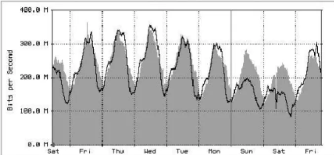
• Traffic Engineering: The TDM tunnels carry IP traffic for hundreds or thousands of users. Traf-fic from large collections of individuals tends to have recurring patterns similar to water or elec-tricity usage corresponding to human’s diurnal cycle, see Figure 1. The TDM tunnels are sized according to peak load (much like the mains electricity supply) and change on a weekly or monthly basis except in the case of emergency
Figure 1: Weekly traffic usage on an OC48 backbone or the automatic fail over of routes. The mil-lisecond routing decisions taken by routers are therefore not needed and a human can make long timescale traffic-engineered decisions over a time period of weeks by monitoring the peak load graphs.
Other authors [9] have realized this cyclical na-ture of the Internet, and the inherent problem [8] with router scalability as Internet traffic continues to grow at a rate of some 100% per year or more [12] – routers apparently do not scale with Moore’s law and they are too slow to accommodate the current rapid growth rates. The authors propose solutions from optical circuit switching [1] to electronic circuit switching on a per TCP flow basis [6, 9]. We contend that this is unnecessary and un-economic.
We suggest that the Internet will be operated most efficiently with a combination of routers for local traf-fic, and TDM tunnels between major traffic centres. The need for core routers that can handle huge vol-umes of traffic can be reduced if we route the bulk of traffic (not destined for that particular node) past the router in TDM pipes. This hybrid (TDM trans-port/packet routing) network conforms to the exist-ing hierarchical design of the Internet and will fur-ther alleviate the N2
problem as the network size increases.
If the hybrid (TDM transport/packet routing) net-work will be with us for the foreseeable future, the question arises: how much headroom does the IP traf-fic inside the TDM transport pipes need in order to realize a given Quality of Service? This question can be answered on many levels, from the technical ideal
to the economic, to the likely practical implementa-tion given past carrier deployment patterns. In this paper we answer the question from the packet delay and packet loss point of view.
2
The simulation experiments
We based our estimate of headroom requirements on a previous simulation for video stream aggrega-tion [2]. In this simulaaggrega-tion the authors used up to 15 MPEG video traces to test the effects of aggregation on video streams. They found that the headroom needed to meet a QoS agreement decreased with in-creasing aggregation. Their results are summarized in Table 1, which agrees with the trend that we ob-serve (Figure 11) although the video traffic seems to need more headroom. This might be because video traffic is more structured than the general Internet traffic that we used in our experiments.
2.1
The sample data
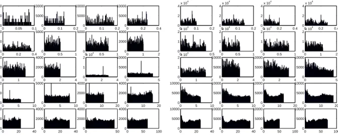
Several traces from NLANR/MOAT [10] were used as the source data for our simulation experiments. These traces represent core traffic collected at differ-ent aggregation points in the Internet. The traces were processed to extract the packet start times in microseconds and the packet lengths in bytes. Several of the traces were examined for anomalies. A class of data (Coral Traces) from the NLANR/MOAT archive was discarded after we determined that nearly all the traces in this class contained a spurious spike of ar-rivals between two and three seconds into the trace. See Figure 2 for an example of one of the anomalous traces.
The traces show packets arriving per second, and number total average % headroom needed of traces bandwidth Mbps for QOS
5 20 150
10 39 85
15 61 58
0 0.05 0.1 0 5000 10000 0 0.1 0.2 0 5000 10000 0 0.1 0.2 0 5000 10000 0 0.2 0.4 0 5000 10000 0 0.2 0.4 0 5000 10000 0 0.5 1 0 5000 0 0.5 1 0 5000 0 1 2 0 2000 4000 0 1 2 0 2000 4000 0 2 4 0 2000 4000 0 2 4 0 1 2x 10 4 0 5 0 5000 10000 0 5 10 0 5000 10000 0 5 10 0 5000 0 10 20 0 2000 4000 0 10 20 0 2000 4000 0 20 40 0 2000 4000 0 20 40 0 2000 4000 0 50 0 2000 4000 0 50 100 0 2000 4000
Figure 2: Anomalous Coral trace
0 0.1 0.2 0 2 4x 10 4 0 0.1 0.2 0 2 4x 10 4 0 0.2 0.4 0 2 4x 10 4 0 0.2 0.4 0 2 4x 10 4 0 0.5 0 1 2x 10 4 0 0.5 1 0 1 2x 10 4 0 0.5 1 0 1 2x 10 4 0 1 2 0 1 2x 10 4 0 1 2 0 1 2x 10 4 0 2 4 0 5000 10000 0 2 4 0 5000 10000 0 5 0 5000 10000 0 5 10 0 5000 10000 0 5 10 0 5000 10000 0 10 20 0 5000 10000 0 10 20 0 5000 10000 0 20 40 0 5000 10000 0 20 40 0 5000 10000 0 50 100 0 5000 10000 0 50 100 0 5000 10000
Figure 3: Bursty but anomaly-free Tsh trace each trace is a collection of 150-point histograms over
larger and larger time intervals. We determined that the data collected in another format (TSH traces) were free of anomalies and we used these traces as our source data. See Figure 3 for an example of the TSH traces.
We used two sets of TSH traces from two different days, Jan 30 2001 and Feb 14 2001. We used a total of fourteen traces from each day, each trace having a timespan of 90 seconds. The average bandwidth of each trace varied from 15 to 70 Mbps, with the average bandwidth of all the traces being 44 Mbps.
2.2
The simulator
Flow aggregation was simulated by inputing the traces to a single FIFO buffer and extracting the packets at a constant rate determined by the output link bandwidth. The FIFO depth and the output link bandwidth could be adjusted. Packets arriving to a full FIFO buffer were discarded. A representation of the switch is shown in Figure 4.
The time between the arrival of a packet and the packet leaving the FIFO was used to measure the de-lay of the packet through the switch. All internal pro-cesses in the switch were assumed to occur with zero delay. The switch was simulated in time units equal
Multiple Queue of packets (one per trace)
fixed length FIFO
Output Link
Figure 4: Simple switch schematic
to the time taken to transmit the minimum packet size (40 bytes) across the output link bandwidth
2.3
The simulation results
We performed various simulation experiments using different levels of aggregation, buffer sizes and output link speeds. We aggregated 2, 4, 6, 8 and 12 traces giving average aggregated bandwidths varying from 35 to 500 Mbps. Initially we used buffer sizes of 4, 8, 16, 32, 64, 128 and 256 Kbytes. For each aggrega-tion level, we determined the average total bandwidth and then increased the output bandwidth to obtain a headroom of 2, 5, 7, 10, 15, 20, 25, 30, 35, 50 and 70%.
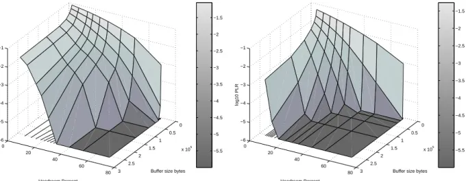
Sample plots of the packet loss ratios at two dif-ferent levels of aggregation are shown in Figures 5
−5.5 −5 −4.5 −4 −3.5 −3 −2.5 −2 −1.5 0 0.5 1 1.5 2 2.5 3 x 10⁵ 0 20 40 60 80 −6 −5 −4 −3 −2 −1
Buffer size bytes Headroom Percent
log10 PLR
Figure 5: Packet loss ratio for an aggregation of 2 traces (35 Mbps) −5.5 −5 −4.5 −4 −3.5 −3 −2.5 −2 −1.5 0 0.5 1 1.5 2 2.5 3 x 10⁵ 0 20 40 60 80 −6 −5 −4 −3 −2 −1
Buffer size bytes Headroom Percent
log10 PLR
Figure 6: Packet loss ratio for an aggregation of 12 traces (491 Mbps)
and 6. The vertical axis displays the logarithm of the packet loss ratio. The x-axis displays the the headroom, namely the spare capacity (100 - percent-age load) of the output link. They-axis displays the buffer size in Mbytes.
Note that the optimal region – the dark floor corre-sponding to low packet loss – is larger for the highly aggregated case (12 flows) than the lightly aggregated case (2 flows). This implies that less headroom is needed to achieve similar packet loss ratios as more flows are aggregated. For example with the largest buffer size of 256 Kbytes, we need a 40% headroom at a bandwidth of 35 Mbps and only a 20% headroom at a bandwidth of 500 Mbps to achieve a packet loss of one in a million.
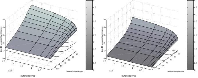
Similar graphs of the average packet delay are shown in Figures 7 and 8. Although the graphs have the same form, we see that the delay is lower for the more aggregated case for the same percentage head-room.
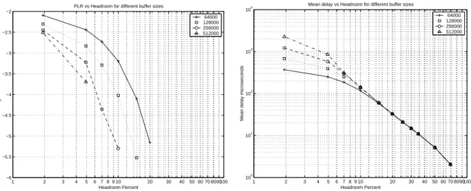
The simulator revealed that smaller buffer sizes gave rise to unacceptable packet losses. Most of the simulation experiments were therefore performed with four buffer sizes namely 64, 128, 256 and 512 Kbytes. The results of these experiments are shown in Figures 9 and 10.
The amount of headroom required by IP traffic de-pends on the QoS criteria applied. We therefore need to specify QoS criteria such as packet loss ratios and packet delays for each class of traffic. Traffic such as real time voice and video streams needs more spare capacity (that is to say, more headroom) than FTP or email traffic. We fixed the packet loss ratio at one in 105
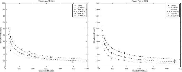
and the average packet delay at 1 msec. These values correspond to an acceptable compressed video stream [2] and they yield the graphs in Figures 11 and 12 which show the headroom required for differ-ent aggregation levels for the two days (Jan 31 and Feb 14 2001) for which traces were collected.
Each graph displays three curves: the lower curve is the average delay, the middle curve is the 95th percentile delay and the top curve is the 99th per-centile delay. On both days and for all three delay measurements (average, 95th and 99th percentile) the headroom follows a power law that decreases with the square root of the bandwidth. The three curves can be represented by the equation
h=ab−p
wherehis headroom needed for the given delay and loss,bis the aggregated average bandwidth in Mbps andaandpare constants wherep∼0.5. A derivation
0 0.5 1 1.5 2 2.5 3 3.5 4 4.5 5 0.5 1 1.5 2 2.5 x 10⁵ 10 20 30 40 50 60 0 1 2 3 4 5 Headroom Percent Buffer size bytes
Log 10 Mean delay microsec
Figure 7: Log average delay for aggregated flows: 2 traces (35 Mbps) 0 0.5 1 1.5 2 2.5 3 3.5 4 4.5 5 0.5 1 1.5 2 2.5 x 10⁵ 10 20 30 40 50 60 0 1 2 3 4 5 Headroom Percent Buffer size bytes
Log 10 Mean delay microsec
Figure 8: Log average delay for aggregated flows: 12 traces (491 Mbps) date delay a p R2 goodness of fit Jan 21 2001 mean 135 0.43 0.93 Jan 21 2001 95th 281 0.54 0.98 Jan 21 2001 99th 308 0.51 0.98 Feb 14 2001 mean 185 0.53 0.96 Feb 14 2001 95th 295 0.56 0.99 Feb 14 2001 99th 317 0.52 0.99
Table 2: Fit results for 1 msec delay, packet loss ratio = 10−5
of the power law in the case where the packet lengths are normally distributed is presented in Section 4.
Table 2 summarizes the results of the fit to the simulation results.
We also performed headroom simulations using more relaxed QoS criteria namely a packet loss ra-tio of one in 104
and a delay constraint of 10 msec. The results are shown in Figure 13. The graph is of the same form as the earlier ones, with two excep-tions: the headroom requirement of 10% is reached at a lower aggregated bandwidth (150 Mbps for the re-laxed constraints vs. 300 to 400 Mbps for the tighter constraints), and the curves for average, 95th
per-date delay a p R2
goodness of fit Feb 14 2001 Mean 141 0.53 0.92 Feb 14 2001 95th 158 0.55 0.95 Feb 14 2001 99th 216 0.59 0.97
Table 3: Fit results for 10 msec delay, packet loss ratio = 10−4
centile and 99th percentile delays nearly coincide. This is because the packet loss constraint dominates over the delay constraint, so the different ways of measuring delay coincide.
2.4
The optimal aggregation point
From the graphs displayed in Figure 11 and Figure 12 (which agree surprisingly well, given that the data were collected two weeks apart), we see that the opti-mal point for aggregating this type of IP traffic with a target packet loss ratio of 1 in 105
and a target delay of 1 msec is around 150 to 200 Mbps. Aggre-gating beyond this level, when we already only need 25% headroom, is in the region of diminishing returns and is not necessary.
1 2 3 4 5 6 7 8 9 10 20 30 40 50 60 70 8090100 −6 −5.5 −5 −4.5 −4 −3.5 −3 −2.5 −2 Headroom Percent Log 10 PLR
PLR vs Headroom for different buffer sizes
64000 128000 256000 512000
Figure 9: Packet loss ratio vs. capacity and buffer size, 12 trace aggregation (550 Mbps) 1 2 3 4 5 6 7 8 9 10 20 30 40 50 60 70 8090100 100 101 102 103 104 Headroom Percent
Mean delay microseconds
Mean delay vs Headroom for different buffer sizes
64000 128000 256000 512000
Figure 10: Mean delay vs. capacity and buffer size, 12 trace aggregation (550 Mbps) 0 100 200 300 400 500 600 0 10 20 30 40 50 60 70 80 90 100 Bandwith Mbit/sec Headroom Percent
Traces Feb 14 2001 Relaxed Contraints
mean fit mean 95th % fit 95th % 99th % fit 99th %
Figure 13: Headroom vs. aggregation level, Feb 14, relaxed constraints
3
The traffic model
It is commonly accepted that Ethernet and Internet traffic is fractal in nature [11]. Such traffic exhibits long-range dependence across many time scales so that aggregating traffic streams does not provide the statistical smoothing that would be expected from random traffic. The Hurst parameter for all the traces was estimated using the slope of the variance vs. the aggregation level [4]. The Hurst parameters for the traces varied in the range 0.77 to 0.89. A Hurst parameter of 0.5 implies random traffic, while Hurst parameters nearer 1 imply traffic that contains bursts over many time scales. Traffic with a Hurst pa-rameter near 1 needs more headroom, as the bursti-ness is not smoothed away by statistical multiplexing. However, there is an advantage to aggregation as the variation in the bandwidth per unit time (the instantaneous bandwidth) declines as we aggregate more streams [5]. Paxton and Floyd [11] showed that the arrival times of the first packet of a flow fits a Poisson model, but that the interarrival times be-tween packets of the same flow are not Poisson but exhibit fractal or self-similar characteristics. How-ever, the interarrival times of many aggregated flows of 50 Mbps and higher are known to follow the the
0 100 200 300 400 500 600 0 10 20 30 40 50 60 70 80 90 100 Bandwith Mbit/sec Headroom Percent Traces Jan 31 2001 mean fit mean 95th % fit 95th % 99th % fit 99th %
Figure 11: Headroom vs. aggregation level Jan31
0 100 200 300 400 500 600 0 10 20 30 40 50 60 70 80 90 100 Bandwith Mbit/sec Headroom Percent Traces Feb 14 2001 mean fit mean 95th % fit 95th % 99th % fit 99th %
Figure 12: Headroom vs. aggregation level Feb 14 Poisson distribution reasonable well [3].
Our sample traces contained over 5000 individual flows, identified by unique source and destination ad-dresses and port numbers. Of these 5000 flows, about 200 flows transmitted over 10 Kbytes during the 90 second trace. The graphs in Figure 14 present the in-terarrival times of short (40 bytes), medium (500-650 bytes) and long (1500 bytes) packets. The graphs on the left of Figure 14 show the number of packets ar-riving in a given interarrival bin (microseconds), and the graphs on the right show the logarithm of the number of packets arriving in a given interarrival bin (microseconds). In each case a spike is observed cor-responding to the bandwidth limit of the incoming pipe (155 Mbit OC3 in this case) followed by a lin-early (in the log case) decreasing tail. These graphs show that the interarrival times are approximately exponentially distributed.
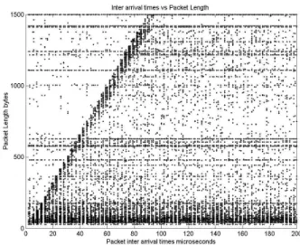
Figure 15 plots the packet lengths vs. the interar-rival times. This graph shows the prominent packet lengths (40, 620 and 1500 bytes) as horizontal bands. The diagonal band gives a link rate of approximately 132 Mbps which represents the cut off limit of the monitored OC3 (155 Mbps) input stream.
The reason that the maximum data rate is 132 Mbps instead of 155 Mbps is due to ATM cell header
−5000 0 500 1000 1500 1
2 3x 10
4
interarrivals microsec short packets trace102
0 200 400 600 800 1000 1 2 3 4 5
log10 interarrivals microsec short packets trace102
−5000 0 500 1000 1500 1000
2000 3000 4000
interarrivals microsec medium packets trace102
0 200 400 600 800 1000 0 1 2 3 4
log10 interarrivals microsec medium packets trace102
−5000 0 500 1000 1500 1 2 3 4x 10 4
interarrivals microsec long packets trace102
0 200 400 600 800 1000 0
2 4 6
log10 interarrivals microsec long packets trace102
Figure 14: Interarrival times for short, medium and long packets
overhead, as these traces were collected on ATM links. Furthermore, there should be no data points to the left of the diagonal band. The fact that such points are present indicate errors in either the trace collection hardware or software. Such errors are well known and are documented in Katabi and Blake [7]. If we re-examine the logarithm plots of the 600 and 1500 byte interarrival times (the lower right two sub-plots of Figure 14) we see that the data points to the left of the spikes at 30 and 90 microseconds are approximately an order of magnitude below their ex-pected value, if we extrapolate the straight line tail back to the time of zero. We chose to omit the “erro-neous” packets in the statistics, as they were an order of magnitude lower than the regular packets.
Figure 15: Packet length vs. interarrival time
4
A simple model
In this Section we describe the flow aggregation pro-cess in terms of a Poisson arrival stream of packets. The average packet length determined as an average of the 15 traces is 612 bytes. The packet average ar-rival rate is thus 0.2042b packets/msec. A random sequence of packet interarrival times was sampled from an exponential distribution with parameter 1/ (0.2042b), and a random sequence of packet lengths
was generated from a tri-modal function that yields a distribution similar to that observed in the real traces as shown in Figure 17.
4.1
The simulation results
Consider the packets which arrive during a time in-terval of say 1 msec. We will evaluate the probability that the data in these packets (header plus payloads bits) divided by the bandwidth of the link is longer than 1 msec.
The following simulation experiments were per-formed. The bandwidth of the output link was varied from 50 to 500 Mbps in steps of 50, and the head-room took the values 10, 20, 30, 40, 50, 75 and 100%. For each (bandwidth, headroom) pair we performed 10,000 experiments. In each experiment we generated a sequence of exponentially distributed packet inter-arrival times. We generated three times as many in-terarrival times as we estimated were needed based on the average packet inter-arrival time. The cumu-lative sum of the packet inter-arrival times yields the simulated arrival time of each packet.
In each experiment, consider the packets which ar-rive during 1 msec. For each arrival we generate a random packet length using the the packet length function that was used to model the observed packet lengths in the traces. The bits that arrived during the 1 msec interval are summed. For each (band-width, headroom) pair we recorded the percentage of the experiments where the arriving bits fitted within the bandwidth.
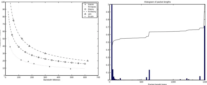
Figure 16 presents the results from (1) simulations using real traces, (2) simulations using exponential packet arrivals, and (3) the headroom power law. The three curves have similar shapes: the simulation pre-dicts a higher headroom than the real traces which is further discussed below.
4.2
Different packet length
distribu-tions
We examined two other packet length distributions:
• constant length packets with length equal to the average of the observed distribution, and
0 100 200 300 400 500 600 700 0 10 20 30 40 50 60 70 80 90 100 Bandwith Mbit/sec Headroom Percent traces fit traces theory fit theory sim fit sim
Figure 16: Headroom for 95% pass vs. bandwidth. Theoretical, simulation and real traces
• packet lengths with a normal distribution with the same mean and variance as the observed packet length distribution.
Constant length packets were observed to have neg-ligable headroom requirements. From this we con-cluded that the main factor contributing to buffer overflow was the packet length variation, and the ex-ponential arrival process contributed only minimally. The normal packet length distribution produced almost identical results to the tri-modal distribution observed with real packet traces. This suggests that the observed statistical gain to be had from aggrega-tion depends only on the mean and standard devia-tion of packet length distribudevia-tion.
4.3
The headroom power law
The simulation results presented in Figures 11, 12 and 13 show that the headroom h follows a power law
h=ab−p
wherebis the bandwidth of the offered traffic in Mbps and a is a constant. The power p is obtained by regression fitting to the traffic data andp∼0.5.
0 500 1000 1500 0 0.1 0.2 0.3 0.4 0.5 0.6 0.7 0.8 0.9 1
Histogram of packet lengths
Packet length bytes
Figure 17: Observed packet length distribution In seeking to explain the power law we observe that the packet length distribution, and hence the mo-ments of the packet length distribution remain con-stant as we aggregate to higher bandwidths.
Let M be a random variable denoting the length of a packet in bits. Assume thatM is normally dis-tributed with mean m and variance σ2
. Consider the random variableB =M1+· · ·+Mn with mean
b=nmand varianceS=nσ2
. If we regardnas the average (rounded up to the nearest integer) number of packets arriving per second, then b is the band-width in bps of the offered traffic.
The additional bandwidthe in bps needed to en-sure that 95% of the offered traffic is transmitted in 1 second isE= 1.64√S. The headroomhis
h=e/b= 1.64√S/b= 1.64σ/√mb.
The measurement from the 15 traces yieldm = 612 andσ= 679 bytes. Substituting these values into the above equation yields
h= 127/√b (1)
Equation (1) is plotted as the circles in Figure 16 and gives a better fit to the observed traces than the simulation model with an exponential packet arrival process and normally distributed packet lengths.
The fact that the simulation results differ from the simulation results when real traffic traces are used can be attributed to the assumption of exponential packet arrivals and also to the fact that no lower bound was placed on the packet length. Real traf-fic is shaped by the absolute hard bandwidth limits of the incoming pipes (for example the 133/155 Mbit limit observed in Figure 15. Further investigation is needed to confirm this.
5
Conclusions
QoS can be defined in terms of packet delay and packet loss. The packet delay can be assumed to be reasonably constant, as it is determined by the ratio of the maximal allowable delay detectable by the human ear/eye divided by the number of jitter-inducing switches that the traffic must cross. We as-sume that 1 msec is an acceptable delay per switch. For toll quality voice telephone conversations a max-imal round trip delay is 300 msec or 150 msec for one way delay [13]. Most one-way trace routes are maximally 15 to 20 hops long. If we assume 40 router hops for a round trip, and allow each router 1 msec of delay, we will be within our delay budget. We must also remember to allow for switching and transmis-sion time in the TDM network which from the G.114 document mentioned above can be calculated as (3 + 0.005×distance in kilometers) msecs.
The packet length distribution can be assumed to stay reasonably constant with time (the only param-eters of the distribution that affect our simulations are the mean and variance). Thus as the total aggre-gated bandwidth increases, we can expect to fit more and more packets into a 1 msec window, and the ad-ditional bandwidth needed to ensure the desired QoS increases with√n wherenis the average number of packets that arrive per second.
Aggregation of IP traffic gives substantial statis-tical multiplexing gains, especially at higher band-widths. TDM tunnels can be sized from the aggregate maximum daily demand using graphs similar to those shown in Figure 1. Network engineers will probably size the tunnels with a safety factor of 100%, as in-stalling new fiber and routers occurs on a timescale
of months.
The conclusions for network design are that we can build simpler, more economical networks by using a collection of cheaper TDM switches to carry fixed bandwidth pipes between major population centers, and fewer and cheaper routers to handle local switch-ing and routswitch-ing in the metro areas.
6
Further Work
Further study is required to determine if the hard shaping of the tributary pipes affects the amount of headroom needed. It might also be useful to do a cost benefit analysis of building a complete network based on TDM switches between major centres with STS1 (50 Mbit) pipe granularity increments and large routers at major cities handling the traffic for that region
Acknowledgments
Thanks to Steve West at Turin Networks for many fruitful discussions, and the encouragement to do this research. Thanks also to Tony Krzesinski at the Uni-versity of Stellenbosch, South Africa for suggestions for improvements to this paper. The traces used for this study were provided by the National Sci-ence Foundation Cooperative Agreement No. ANI-9807479, and the National Laboratory for Applied Network Research
References
[1] Bannister, J.J. Touch, A. Willner, and S. Suryaputra,How Many Wavelengths Do We really Need? A Study of the Performance Limits of Packet Over Wavelengths,
SPIE/Baltzer Optical Networks, Vol. 1, No. 2, Feb. 2000, pp. 17-28.
[2] B. Bashforth and C. Williamson,Statistical Multiplexing of Self Similar Video Stream: Simulation Study and Performance Results, Modeling, Analysis and Simulation of
Computer and Telecommunication Systems 1998
[3] J. Cao, W.S. Cleveland, D. Lin, and D.X. Sun,
Internet Traffic Tends Toward Poisson and Independent as the Load Increases, Nonlinear Estimation and Classification , Eds. C. Holmes, D. Denison, M. Hansen, B. Yu, and B. Mallick, Springer, New York, 2002.
[4] Y. Chen, Z. Deng and C. Williamson,A Model for Self-Similar Ethernet LAN Traffic: Design, Implementation, and Performance
Implications, Proceedings of the 1995 Summer Computer Simulation Conference (SCSC’95), Ottawa, Ontario, pp. 831-837, July 1995. [5] A. Erramilli, W. Willinger,A case for fractal
traffic modeling, Second Australian
Telecommunication and Network Applications Conference ‘96, Sydney, December 1996. [6] A.Feldmann, J.Rexford, and R.Caceres.
Efficient policies for carrying web traffic over flow-switched networks. In IEEE/ACM Transactions on Networking, pp. 673–685, December 1998.
[7] D. Katabi and C. Blake.Inferring Congestion Sharing and Path Characteristics for Packet Interarrival times. MIT-LCSTR -828, December 2001.
[8] N. McKeown,Weren’t routers supposed to be simple? ICSI informal talk, May 2002. [9] P. Molinero-Fernandez and N. McKeownTCP
Switching: Exposing circuits to IP, IEEE Micro, January 2002
[10] The National Laboratory for Applied Network Research (NLANR),
http://moat.nlanr.net/Traces/
[11] V. Paxson and S. Floyd,Wide-area Traffic: The Failure of Poisson Modeling,IEEE/ACM Transactions on Networking, pp.226-244, June 1995.
[12] J. Roberts et al., 2001. US Internet Traffic 8-15-2001, c2001 Caspian Networks, Inc. http://www.caspiannetworks.com/library/ presentations/traffic/
Internet Traffic 011602.ppt
[13] ITU-T recommendation G.114, One-way transmission time, (05/00) Approved 2000-05.