Evaluation of ensemble NWP models for dynamical downscaling of air temperature over complex topography in a hot climate: A case study from the Sultanate of Oman

(1)

Evaluation of ensemble NWP models for dynamical downscaling of air

temperature over complex topography in a hot climate: A case study from the

Sultanate of Oman

YASSINE CHARABI

Department of Geography, Sultan Qaboos University, Oman

Corresponding author; e-mail: [email protected]

SULTAN AL-YAHYAI

Department of Information Technology, Mazoon Electricity Company, Oman

Received: January 16, 2014; accepted: August 5, 2015

RESUMEN

Este trabajo evalúa el uso de modelos numéricos de predicción del tiempo (NWP, por sus siglas en inglés) por conjuntos para la reducción dinámica de escala de la temperatura en una región cálida y compleja. Este enfoque ofrece información sobre la incertidumbre de los modelos NWP y proporciona información probabilística para compararlos con los modelos NWP sencillos que se utilizan en la actualidad. Se construyó un sistema por conjuntos utilizando cuatro partes con una resolución de 7 km sobre Omán. Dichas partes estuvieron conformadas por dos modelos de área limitada (LAM, por sus siglas en inglés), el modelo de alta resolución y el modelo del Consorcio para la Modelación de Pequeña Escala. Los dos LAM se derivaron e inicializaron utilizando datos del modelo de circulación general del modelo global alemán, que opera con una resolución de 40 km con base en dos estados atmosféricos iniciales. El primer estado inicial fue proporcionado por el sistema de asimilación de datos 3Dvar del Servicio Meteorológico Alemán, y el segundo estado inicial se obtuvo a partir de los datos de reanálisis (ERA-Interim) del Centro Europeo para la Predicción del Tiempo

con la incertidumbre de los modelos NWP utilizados, e indican que no hay un modelo idóneo para la totalidad del dominio. En general, el promedio del conjunto tuvo un mejor desempeño que las partes individuales.

ABSTRACT

This paper evaluates the use of ensemble numerical weather prediction (NWP) models for dynamical down-scaling of temperature over a complex, hot region. This approach delivers information about the uncertainty of the NWP models and provides probabilistic information for comparison with the currently used single NWP model. An ensemble system was constructed using four members with a 7 km resolution over Oman. Two limited-area models (LAMs), the high-resolution model (HRM) and the model from the Consortium for Small-Scale Modeling (COSMO) formed the ensemble members. The two LAMs were derived and initialized using the general circulation model (GCM) data from the German Global Model (GME), which

by the 3Dvar data assimilation system at the German Weather Service (Deutscher Wetterdienst, DWD), and the second initial state was provided from the reanalysis data (ERA-Interim) from the European Centre for Medium-Range Weather Forecasts (ECMWF). The results reveal the uncertainty in temperature prediction related to the uncertainty of the NWP models that were used and indicate that there is no best model for the entire domain. On average, the ensemble mean performed better than individual members.

Keywords: Dynamical downscaling, ensemble NWP models, temperature, complex hot area.

(2)

1. Introduction

Over the last decade, the availability of increasing computing power has supported concerted efforts to improve the resolution of numerical weather prediction

(NWP) models (Ruby Leung et al., 2003). Despite

these efforts, the resolution of NWPs remains coarse. The typical resolution ranges from a few dozen kilo-meters for general circulation models (GCMs) down to a few kilometers for limited-area models (LAMs)

(Eccel et al., 2007). The air temperature at 2 m above

the ground is one of the main meteorological parame-ters forecasted by NWP models, but this prediction is closely tied to the topographic position assigned by the model to each grid point. Air temperature is strongly affected by topography, and large-scale models can be a source of strong bias in complex terrain. The lowest model layer is much higher than 2 m, adding to the bias introduced by the horizontal resolution. Therefore, the 2 m temperature is not a prognostic model vari-able but is interpolated from the lowest model layer. The type of interpolation will contribute to the bias in the forecasted 2 m temperature compared with the measured one. Therefore, a downscaling approach is

used as a post-processing step for deriving finer reso -lution information from large-scale NWP models and to relate grid point predictions to the actual physical

sites (Hewitson and Crane, 1996; Eccel et al., 2007).

There are two principal types of downscaling techniques: statistical/probabilistic and dynamical. Statistical/probabilistic downscaling methods use his-torical data and archived forecasts to generate down-scaled data from large-scale forecasts (Murphy, 1998; Rummukainen, 2010). Statistical downscaling consists in identifying empirical links between large-scale patterns of climate elements (predictors) and local climate (the predictands), and applying them to output from global or regional models. This approach is very

simple to implement, fits well with areas with large

datasets and generates consistent estimates for periods similar to those used for their calibration. Successful downscaling depends on long, reliable observational series of predictors and predictands.Dynamical down-scaling methods encompass dynamic models of the atmosphere nested within the grids of the large-scale forecast models. Typically, one-way nested LAMs are

implemented to generate finer resolutions for different

applications, with GCMs providing initial and lateral boundary conditions. Dynamic downscaling has be-come very popular; the physical model formulation

offers strong justification for its application under a

variety of climate and weather conditions, particularly for locations with strong boundary forcing, such as complex terrain with irregular orography (Murphy, 1998; Rummukainen, 2010). The disadvantage of this approach is related to the high computational cost and data requirements (e.g., three dimensional boundary and initial conditions).

Statistical and dynamic downscaling techniques have been used, separately or combined, in meteorol-ogy and hydrolmeteorol-ogy to improve understanding of local

climate variability (Al-Yahyai et al., 2011; Burger,

1996; Fowler et al., 2007; Fuentes and Heimann, 2000;

Haas and Born, 2011; Hubener and Kerschgens, 2007;

Kidson and Thompson, 1998; Maraun et al., 2010;

Michelangeli et al., 2009; Pinto et al., 2010; Wilby

et al., 1998; Wilby and Wigley, 1997). Ensemble ap-proaches were introduced in meteorology (Galmarini et al., 2001) and hydrology (Stedinger and Kim, 2009) to improve model forecasts and reduce the model uncertainty. Any group of model forecasts with the same valid time is called an ensemble (UCAR, 2009), and each forecast is called an ensemble member. The extent of agreement among the members can be considered a measure of forecast certainty (Stensrud et al., 1999). Ensemble forecasting can quantify and propagate forecast uncertainty (Tiwari and Chatterjee, 2010; National Research Council, 2006).

The implementation of downscaling techniques in developing countries poses a real challenge due to the modest computational infrastructure. The main motivation of this study is to construct an ensemble of forecasts over a complex, hot area. Several techniques for constructing the ensemble have been developed and exhibit better performance than any single model

system (Callado et al., 2013). The proposed

method-ology suggests using various sources of NWP model uncertainty as a starting point to generate an ensemble of NWP predictions for temperature data. This meth-od can be achieved by using different LAMs (initial/ boundary) derived by different GCMs. The Sultan-ate of Oman, characterized by a hyper-arid climSultan-ate because of its position astride the tropic of Cancer, was selected as a reference area for this application (Fig. 1). The rainfall regime, the teleconnections and the wet- and dry-spell patterns have been analyzed on a regional scale in this region (Charabi, 2009; Charabi and Hatrushi, 2010; Charabi and Al-Yahyai, 2011).

(3)

different atmospheric mechanisms which contribute to local climate diversity and that are characterized by a strong gradient of temperature induced by the complexity of the topography. There are no studies of this region that address the interaction between such complex topography and temperature at local scales. The outline of the paper is as follows: section 2 details the proposed approach; section 3 discusses the

main findings based on a case study over Oman; and

section 4 concludes the paper.

2. Data sets and methodology

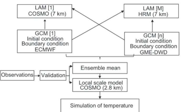
Figure 2 gives a comprehensive overview of the ensemble NWP model approach for dynamical downscaling of temperature. It shows that initial and lateral boundary conditions from [M] GCMs (40 × 40 km) are used to derive and initialize [N] LAMs (7 × 7 km). This permutation generates an ensemble system [M × N] member. In this combination, each LAM will be initialized by [M] different GCMs. The models are equally weighted, meaning the ensemble

members for each model are calculated first and then

averaged to form the multi-model mean. This regional scale ensemble prediction is validated with the ground observations and used to derive and initialize a local scale high-resolution model (2.8 × 2.8 km). Notice that the number of ensemble members is controlled by the

availability of the GCMs data and the computational power. The higher the number of members, the more

confident the derived statistics but the more computa

-tional power required (Al-Yahyai et al., 2011). For this

application, an ensemble system was constructed using four members and covering the domain 49.0-64.0º E and 13.0-28.0º N with a 7 km resolution with 241 × 241 grid points and 41 vertical layers. Two LAMs, namely the high-resolution model (HRM), which is hydrostatic (Majewski, 2009), and the model from the Consortium for Small-Scale Modeling (COSMO), which is non-hydrostatic (Doms and Schattler, 2008), formed the ensemble members.

Each model run is initialized at 00:00 UTC and

generates output for 30 hours. The first six hours are

discarded due to the spin-up of the model. The two LAMs are derived and initialized by the GCMs’ data from the German Global Model (GME), which runs at 40 km resolution using two different initial states of

the atmosphere. The first initial state of the atmosphere

is provided by the 3Dvar data assimilation system at the German Weather Service (Deutscher Wetterdienst, DWD), and the second initial state is provided from the reanalysis data ERA-Interim from the European Cen-tre for Medium-Range Weather Forecasts (ECMWF, 2006). The HRM model has been an operational model at the Directorate General of Meteorology and Air Nav-igation (DGMAN), Oman, since 1999. The COSMO model has recently been implemented as a test bed under the research agreement between DGMAN and DWD. Through this cooperative agreement, DWD provided the initial and lateral boundary conditions for 2009 for this study; the study therefore covers only 2009. The PC cluster of the DGMAN was used to run the case study after the operational runs of its operational models.

Latitude N (º

)

27

26

25

24

23

22

21

20

19

18

17

16

Longitude E (º)

2400

2200 2000

1600

1400

1200

800

600 500

300

200

100

52 53 54 55 56 57 58 59 60 61

Fig. 1. 2.8 km averaged elevation (m) of the study area.

GCM [n] Initial condition Boundary condition

GME-DWD LAM [1]

COSMO (7 km) HRM (7 km)LAM [M]

GCM [1] Initial condition Boundary condition

ECMWF

Ensemble mean Local scale model

COSMO (2.8 km) Validation

Observations

Simulation of temperature

(4)

3. Results and discussion

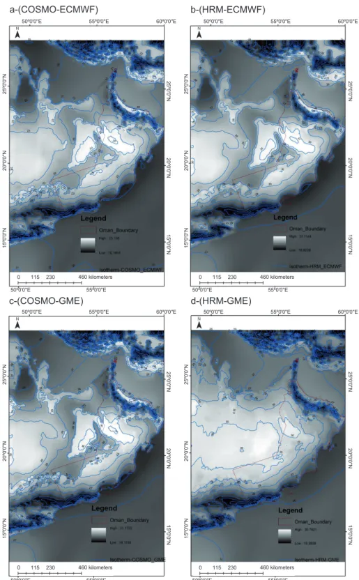
Figure 3 shows the annual mean temperature at 2 m above the ground from the four ensemble members. This figure shows the uncertainty of the NWP models

a-(COSMO-ECMWF)

25º0'0''N

50º0'0''E 55º0'0''E 60º0'0''E

50º0'0''E 55º0'0''E

20º0'0''N

15º0'0''N

25º0'0''N

20º0'0''N

15º0'0''N

b-(HRM-ECMWF)

N

460 kilometers 0 115 230

25º0'0''N

50º0'0''E 55º0'0''E 60º0'0''E

50º0'0''E 55º0'0''E

20º0'0''N

15º0'0''N

25º0'0''N

20º0'0''N

15º0'0''N

N

c-(COSMO-GME) d-(HRM-GME)

25º0'0''N

50º0'0''E 55º0'0''E 60º0'0''E

50º0'0''E 55º0'0''E

20º0'0''N

15º0'0''N

25º0'0''N

20º0'0''N

15º0'0''N

N

25º0'0''N

50º0'0''E 55º0'0''E 60º0'0''E

50º0'0''E 55º0'0''E

20º0'0''N

15º0'0''N

25º0'0''N

20º0'0''N

15º0'0''N

N

(5)

and illustrates the effects of model dynamics, numerical schemes and the initial conditions. The HRM-DWD and COSMO-DWD maps clearly highlight the effect of the model dynamic and numerical schemes. The two LAMs are initialized with the same atmospheric states engendered in two different forecasts. The effect of the initial state is clearly shown, with maps of the same model (e.g. HRM) using different initial states engen-dering two different forecasts. Notice that the effects of the model dynamics and numerical schemes are more pronounced than the effect of the initial state. It can be seen that the HRM model is more sensitive to the initial and boundary condition data than the COSMO model. The HRM model initialized by the DWD 3D data assimilation produced high temperatures over the Empty Quarter desert.

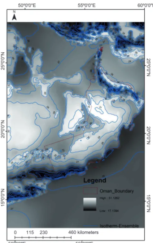
Figure 4 shows the annual ensemble mean of the system. The ensemble mean smoothed out the unpredictable events, such as the high temperature over the Empty Quarter desert. On the other hand, the more predictable events, such as low air tem-perature over the mountains, were maintained in the ensemble mean.

Eleven meteorological stations were selected to verify the robustness of the temperature simulation

of the four ensemble members and the ensemble mean against ground observations. Figure 5 shows the scatter plot for different forecasts over Salalah. In most cases, the model underestimated the low temperature values and overestimated the high temperature values. Therefore, the NWP models have warm and cold biases over Salalah. Due to the variation in bias of the models, the ensemble mean showed outliers in the scatter plot. Monthly time se-ries of the mean temperature were also computed. The diagram at the lower right corner shows the model validation data over Salalah against the observation data (black curve). All models underestimated the temperature during winter and overestimated the tem-perature during summer. The model discrimination over Salalah is believed to be related to the complex terrain surrounding the observational station and the large seasonal temperature variation. The southern

part of Oman, where Salalah is located, is influenced

by the Arabian summer monsoon from June to Sep-tember, which considerably reduces the temperature. Compared with Salalah, the scatter plot over Sohar shows a better correlation with the measurement observations, as shown in Figure 6. Similar results from the ensemble mean model were observed for the other stations.

The mean error (bias) of the four ensemble mem-bers and the ensemble mean is calculated as described by Eq. (1):

i N

i O

F N Bias=

∑

−

i=1

1 ₍₁₎

where F is the model forecast, O is the observation and N is the total number of data sets.

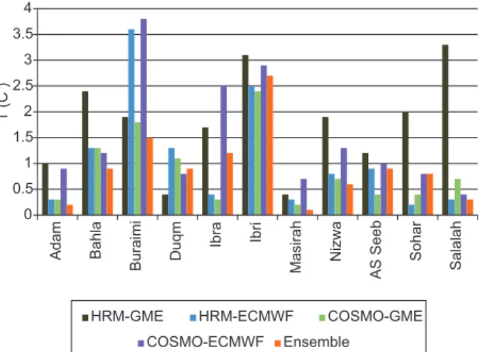
The mean error is determined from the means of the closest points of the model to an observational station and the bi-linearly interpolated value of the four surrounding points. Figure 7 shows the mean error (bias) of the four ensemble members, the mean error of the ensemble mean using the closest grid point approach and the bi-linear interpolation of the four surrounding grid points for eleven meteorolog-ical stations. It clearly shows that all members are overestimating the temperature for all stations by 1-3.5 ºC. The highest overestimation is shown in

Buraimi and Ibri. This significant difference can be

explained by the topographic divergence between

Fig. 4. Annual mean temperature at 2 m above the ground from the ensemble mean.

25º0'0''N

50º0'0''E 55º0'0''E 60º0'0''E

50º0'0''E 55º0'0''E

20º0'0''N

15º0'0''N

25º0'0''N

20º0'0''N

15º0'0''N

N

(6)

0 10 20 30 40 50

10 30 50

T (C) Observe

d

T (C) Forecasted

0 10 20 30 40 50

T (C) Observe

d

T (C) Forecasted 0

10 20 30 40 50

0 10 20 30 40 50

T (C) Observe

d

T (C) Forecasted 0

10 20 30 40 50

0 10 20 30 40 50

T (C) Observe

d

T (C) Forecasted

0 10 20 30 40 50

T (C) Observed

T (C) foracasted

a-Temperature HRM-GME b-Temperature-HRM-ECMWF

c-Temperature COSMO-GME d-Temperature COSMO-ECMWF

d-Temperature -Ensemble

20 22 24 26 28 30 32

Jan Feb Mar Apr May Jun Jul Aug Sep Oct Nov Dec

T (C

)

T_hrm_gme T_hrm_ecmwf T_cosmo_gme

T_cosmo_ecmwf T_ensemble T_obs

f-(Comparisonofensemble members,ensemble mean and observed monthly mean time series)

Fig. 5. Verification results for the Salalah station scatter plots for different forecasts: (a) T

(7)

0 10 20 30 40 50 60

0 10 20 30 40

T (C ) Observed

T (C ) Forecasted a-Temperature HRM-GME

0 10 20 30 40 50 60

0 10 20 30 40

T (C ) Observed

T (C ) Forecasted

0 10 20 30 40 50 60

0 10 20 30 40

T (C ) Observe

d

T (C ) Forecasted

0 10 20 30 40 50 60

0 10 20 30 40

T (C) Observation

T (C) Forecasted

0 10 20 30 40 50 60

0 10 20 30 40

T (C) Observation

T (C) Forecasted

b-Temperature HRM-ECMWF

c-Temperature COSMO-GME

e-Temperature Ensemble

d-Temperature COSMO-ECMWF

18 23 28 33 38

Jan Feb Mar Apr May Jun Jul Aug Sep Oct Nov Dec

T (C

)

T_hrm_gme T_hrm_ecmwf T_cosmo_gme

T_cosmo_ecmwf T_ensemble T_obs

f-Comparison of ensemble members, ensemble mean and observed monthly mean time series

Fig. 6. Verification results for the Sohar station scatter plots for different forecasts. (a) T

(8)

the elevation of the station and the elevation per-ceived by the model. For these two stations, the difference is more than 100 m. Moreover, these differences in temperatures may be related to plan-etary boundary layer (PBL) heights. PBL heights are underestimated in those regions, which may be a result of differences in land cover between our downscaling models data set and the ground-truth data. Furthermore, Burimi and Ibri are highly

in-fluenced by the strong sea breeze blowing from the

northeast coast of the United Arab Emirates. This

deep penetration of sea breezes over a large flat area

contributes to a reduction in the air temperature (Charabi and Al-Yahyai, 2011).

Among the four members and the mean error of the ensemble mean, HRM-GME performed better for Duqum; HRM-ECMWF performed better in the case of Sohar; and Ibra, Ibri and As Seeb were forecasted better by COSMO-GME. Adam, Buraimi, Masirah, Nizwa, and Salalah were forecasted better by the en-semble mean. These results highlight the uncertainty of the NWP model and show that there is no best model for the entire domain. The bi-linear approach indicated that the ensemble mean performed better for six stations.

4. Conclusion

This paper assesses the use of ensemble NWP models for dynamical downscaling of temperature over a complex hot area. The results show the uncertainty in temperature prediction due to the uncertainties in the NWP models that were used and indicate that

there is no best model for the entire domain. The NWP models performed relatively poorly in pre-dicting temperature; this is mainly because the NWP

models reliance on simple soil physics is insufficient

to capture the temperature cycle over the different topographic settings. The multilayer soil model used in NWP models mainly simulates soil temperature evolution; soil vegetation, humidity and canopy are based on seasonal variations in land cover and are not explicitly computed. In Oman, accurate topo-graphical information and advanced surface physics are required to improve temperature prediction. Therefore, soil hydrological models and plant cano-py models are important for realistic assessments of evaporation, evapotranspiration and their impacts on

the latent and sensible surface heat fluxes that directly influence the air temperature.

¡The ensemble mean performed better on aver-age than individual members. The atmosphere is a chaotic system, where predictability is lost in a

manner-dependent flow; providing a single control

forecast is of limited use. An ensemble approach, where multiple predictions are generated through initial and model perturbations, can be used to assess variations in predictability and substantially reduce the uncertainty.

Acknowledgments

The authors would like to acknowledge The Research Council of Oman (Grant RC/ENG/ECED/10/01) for funding this research and the Directorate General of Meteorology and Air Navigation (DGMAN) for providing access to run the simulation on their high performance PC Cluster machine and for providing the observational data for the model validation.

References

Al-Yahyai S., Y. Charabi, A. Al-Badi and A. Gastli, 2011. Nested ensemble NWP approach for wind energy as-sessment. Renew. Energ.37, 150-160, doi:10.1016/j. renene.2011.06.014.

Burger G., 1996. Expanded downscaling for generating local weather scenarios. Clim. Res.7, 111-128. Callado A., P. Escribà, J. A. García-Moya, J. Montero, C.

Santos, D. Santos-Muñoz and J. Simarro, 2013. En-semble forecasting. In: Climate change and regional/ local responses (Y. Zhang and P. Ray, Eds.). Intech. Available at: http://www.intechopen.com/books/cli-mate-change-and-regional-local-responses.

Fig. 7. Mean error (bias) of the ensemble members at different locations.

0 0.5 1 1.5 2 2.5 3 3.5 4

Adam Bahla

Buraim

i

Duqm Ibra Ibri

Masira

h

Nizw

a

AS Seeb Sohar Salalah

T (C

)

(9)

Charabi Y. and S. Al-Hatrushi, 2010. Synoptic aspects of winter rainfall variability in Oman. Atmos. Res.95, 470-486, doi:10.1016/j.atmosres.2009.11.009. Charabi Y. and S. Al-Yahyai, 2011. Integral assessment

of air pollution dispersion regimes in the main indus-trialized and urban areas in Oman. Arabian Journal of Geosciences 3-4, 625-634, doi:10.1007/s12517-010-0239-6.

Doms G. and U. A. Schattler, 2008. A description of the nonhydrostatic regional model LM. Part I: Dynamics and numerics. Deutscher Wetterdienst, Germany. Eccel E., L. Ghielmi, P. Granitto, R. Barbiero, F. Grazzini

and D. Cesari, 2007. Prediction of minimum tem-peratures in an alpine region by linear and non-linear post-processing of meteorological models. Nonlinear Proc. Geophys. 14, 211-222, doi:10.5194/npg-14-211-2007.

ECMWF, 2006. Newsletter No. 110. European Centre for Medium-Range Weather Forecasts.

Fuentes U. and D. Heimann, 2000. Review: An improved statistical dynamical downscaling scheme and its appli-cation to the Alpine precipitation climatology. Theor. Appl. Climatol.65, 119-135.

Fowler H. J., S. Blenkinsopa and C. Tebaldib, 2007. Review: Linking climate change modelling to impacts studies: Recent advances in downscaling techniques for hydro-logical modelling. Int. J. Climatol.27, 1547-1578. Galmarini S., R. Bianconi, R. Bellasio and G. Graziani,

2001. Forecasting the consequences of accidental releases of radionuclides in the atmosphere from en-semble dispersion modelling. J. Environ. Radioactiv.

57, 203-219.

Haas R. and K. Born, 2011. Probabilistic downscaling of precipitation data in a subtropical mountain area: A two-step approach. Nonlin. Processes Geophys. 18, 223-234, doi:10.5194/npg-18-223-2011.

Hewitson B. C. and R. G. Crane, 1996. Climate down-scaling: Techniques and application. Clim. Res. 7, 85-95.

Hubener H. and M. Kerschgens, 2007. Downscaling of current and future rainfall climatologies for southern Morocco. Part I: Downscaling method and current climatology. Int. J. Climatol.27,1763-1774.

Kidson J. W. and C. S. Thompson, 1998. A comparison of statistical and model-based downscaling techniques for estimating local climate variations. J. Climate11, 735-753.

Majewski D., 2009. HRM user’s guide. Deutscher Wet-terdienst, Germany.

Maraun D., F. Wetterhall, A. M. Ireson, R. E. Chandler, E. J. Kendon, M. Widmann, S. Brienen, H. W. Rust, T. Sauter, M. Themeßl, V. K. C. Venema, K. P. Chun, C. M. Goodess, C. M. Jones, C. Onof, M. Vrac and I. Thiele-Eich, 2010. Precipitation downscaling under climate change: Recent developments to bridge the gap between dynamical models and the end user. Rev. Geophys.48, RG3003, doi:10.1029/2009RG000314. Michelangeli P. A., M. Vrac and H. Loukos, 2009. Proba-bilistic downscaling approaches: Application to wind cumulative distribution functions. Geophys. Res. Lett.

36, L11708, doi:10.1029/2009GL038401.

Murphy J., 1998. An evaluation of statistical and dy-namical techniques for downscaling local climate. J. Climate12, 2256-2284.

National Research Council, 2006. Completing the forecast: Characterizing and communicating uncertainty for better decisions using weather and climate forecasts. National Academy Press, Washington, DC, 124 pp. Pinto J. G., C. P. Neuhaus, G. C. Leckebusch, M. Reyers and

M. Kerschgens, 2010. Estimation of wind storm impacts over West Germany under future climate conditions us-ing a statistical dynamical downscalus-ing approach. Tellus A62, 188-201, doi:10.1111/j.1600-0870.2009.00424.x. Ruby Leung L., L. O. Mearns, F. Giorgi and R. L. Wilby,

2003. Regional climate research: Needs and opportu-nities. B. Am. Meteorol. Soc.84, 89-95, doi:10.1175/ BAMS-84-1-89.

Rummukainen M., 2010. State-of-the-art with regional climate models. WIREs Clim. Change1, 82-96. Stedinger J. R. and Kim Y., 2009. Probabilities for

en-semble forecasts reflecting climate information. J. Hydrol. 391, 9-23.

Stensrud D. J., H. E. Brooks, J. Du, M. S. Tracton and E. Rogers, 1999. Using ensembles for short-range fore-casting. Mon. Weather Rev.127, 433-446.

Tiwari M. K. and C. Chatterjee, 2010. Uncertainty

assess-ment and ensemble flood forecasting using bootstrap based artificial neural networks (BANNs). J. Hydrol.

382, 20-33.

UCAR, 2009. Introduction to ensemble prediction (online). University Corporation for Atmospheric Research, Boul-der, Co.Wilby R. L. and T. M. L. Wigley, 1997. Down-scaling general circulation model output: A review of methods and limitations. Prog. Phys. Geog.21, 530-548. Wilby R. L., T. M. L. Wigley, D. Conway, P. D. Jones, B.

C. Hewitson and D. S. Wilks, 1998. Statistical down-scaling of GCM output: A comparison of methods.