Published online July 30, 2014 (http://www.sciencepublishinggroup.com/j/ajnc) doi: 10.11648/j.ajnc.s.2014030501.12
ISSN: 2326-893X (Print); ISSN: 2326-8964 (Online)
Complex performance modeling of parallel algorithms
Peter Hanuliak, Juraj Hanuliak
Dubnica Technical Institute, Sladkovicova 533/20, Dubnica nad Vahom, 018 41, Slovakia
Email address:
[email protected] (P. Hanuliak)
To cite this article:
Peter Hanuliak, Juraj Hanuliak. Complex Performance Modeling of Parallel Algorithms. American Journal of Networks and
Communications. Special Issue: Parallel Computer and Parallel Algorithms. Vol. 3, No. 5-1, 2014, pp. 15-28.
doi: 10.11648/j.ajnc.s.2014030501.12
Abstract:
Parallel principles are the most effective way how to increase parallel computer performance and parallel algorithms (PA) too. In this sense the paper is devoted to a complex performance evaluation of chosen PA. At first the paper describes very shortly PA and then it summarized basic concepts for performance evaluation of PA. To illustrate the analyzed evaluation concepts the paper considers in its experimental part the results for real analyzed examples of discrete fast Fourier transform (DFFT). These illustration examples we have chosen first due to its wide application in scientific and engineering fields and second from its representation of similar group of PA. The basic form of parallel DFFT is the one-dimensional (1-D), unordered, radix–2 algorithm which uses divide and conquer strategy for its parallel computation. Effective PA of DFFT tends to computing one – dimensional FFT with radix greater than two and computing multidimensional FFT by using the polynomial transfer methods. In general radix - q DFFT is computed by splitting the input sequence of size s into q sequences each of them in size n/q, computing faster their q smaller DFFT’s, and then combining the results. So we do it for actually dominant asynchronous parallel computers based on Network of workstations (NOW) and Grid systems.Keywords:
Parallel Computer, NOW, Grid, Parallel Algorithm (PA), Matrix PA, Decomposition, Performance Modeling,Optimization, Issoeficiency Function, Numerical Integration, Discrete Fast Fourier Transform (DFFT), Overhead Function
1. Introduction
Parallel and distributed computing has been evolved as two separate research disciplines. Parallel computing has addressed problems of communication and intensive computation on highly-coupled computing nodes while distributed computing has been concerned with coordination, availability, timeliness, etc., of more likely coupled computing nodes. Current trends, such as parallel computing on networks of high performance computing nodes (workstations) and Internet computing, suggest the advantages of unifying these two research disciplines. In relation to these trends we have developed a flexible model of computation that supports both parallel and distributed computing [11].
Parallel and distributed computing share the same basic computational model consisting on physically distributed parallel processes that operate concurrently and interact with each other in order to accomplish a task as a whole. In parallel computing, processes are assumed to be placed closer to each other and they could communicate frequently
and hence the ratio of computation/communication of parallel applications is usually much smaller than that in distributed applications. On the other hand, distributed computing focuses on parallel processes that could be allocated in a wide area i. e., communication between some parallel processes is assumed to be more costly than in parallel computing.
efficiently. Another important trend is a convergence of parallel and distributed computing is the potential of Internet computing. With improvements in network technology and communication middleware, one can view the Internet as a huge of parallel and distributed computers. Because connectivity on the Internet can be intermittent variable of the bandwidth, the ability of processes as well as data to migrate becomes critical. In turn, this requires a satisfactory treatment of mobility.
2. Architectures of Parallel Computers
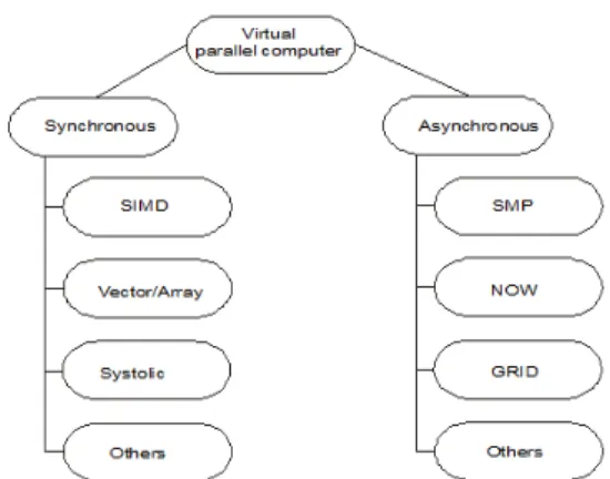
It is very difficult to classify all existed parallel computers. We have tried to classify them from the point of program developer [1, 9] to the two following basic groups according Figure1.
• synchronous parallel computers. They are often used under central control, that means under the global clock synchronization (vector, array system etc.) or a distributed local control mechanism (systolic systems etc.). The typical architectures of this group of parallel computers illustrate Figure 1 on its left side
• asynchronous parallel computers. They are composed of a number of fully independent computing nodes (processors, cores, and computers). To this group belong mainly various forms of computer networks (cluster), network of workstation (NOW) or more integrated Grid modules based on NOW modules. The typical architectures of asynchronous parallel computers illustrate Figure 1 on its right side.
Figure 1. Suggested classification of parallel computers.
2.1. Dominant Parallel Computers
2.1.1. Network of Workstations
There has been an increasing interest in the use of networks (Cluster) of workstations connected together by high speed networks for solving large computation intensive problems [5]. This trend is mainly driven by the cost effectiveness of such systems as compared to massive multiprocessor systems with tightly coupled processors and memories (Supercomputers). Parallel computing on a cluster of workstations connected by high speed networks has given rise to a range of hardware and network related issues on any
given platforms [15, 26]. Load balancing, inter processor communication (IPC), and transport protocol for such machines are being widely studied [20, 21].
This trend is mainly driven by the cost effectiveness of such systems as compared to massive multiprocessor systems with tightly coupled processors and memories (Supercomputers). With the availability of high performance personal computers (workstation) and high speed communication networks (Infiniband, Quadrics, Myrinet), recent trends are to connect a number of such workstations to solve complex problems in parallel on such NOW modules [24, 28].
Figure 2. Illustration of NOW.
Principal example of NOW module is at Figure 2. The individual workstations PCi are mainly powerful
workstations based on symmetrical multiprocessor or multicore platform (SMP).
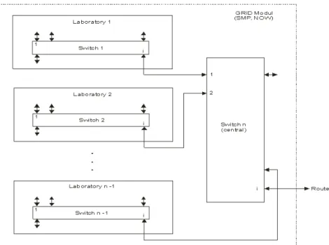
2.1.3. Grid Systems
Grid represents a new way of managing and organizing of individual resources (processors, memory modules, I/O devices etc.) [33]. Grids go out conceptually from a structure of virtual parallel computer based on NOW modules. We have illustrated at Figure 3 typical integrated Grid module based on NOW modules. Any classic parallel computer (massive multiprocessors as supercomputers etc.) could be a member of any NOW module [29].
3. Parallel Algorithms
In principal we can divide parallel algorithms (PA) to the following groups
• parallel algorithm using shared memory (PAsm). These
algorithms are developed for parallel computers with shared memory as actual modern symmetrical multiprocessors (SMP) or multicore systems on motherboard
• parallel algorithm using distributed memory (PAdm).
These algorithms are developed for parallel computers with distributed memory as actual NOW system and their higher integration forms named as Grid systems • hybrid PA which combine using of both previous PA
(PAhyb). This trend support applied using of NOW
Figure 3. Grid as integration of NOW network.
The main difference between PAsm and PAdm is in form
of inter process communication (IPC) among created parallel processes [12, 17]. Generally we can say that IPC communication in parallel system with shared memory can use more communication possibilities (all the possibilities of communication in shared memory) than in distributed systems (only network communication).
3.1. Developing Process of PA
The role of programmer is for the given parallel computer and for given application problem to develop the effective parallel algorithm. This task is more complicated in those cases, in which we have to create the conditions for any parallel activities in form of dividing the sequential algorithm to their mutual independent parts named parallel processes. Principally development of any parallel algorithms (shared memory, distributed memory) includes following activities [10, 18].
• decomposition - the division of the application problem into a set of parallel processes and their data • mapping - the way how created parallel processes and
data are distributed among the nodes of parallel computer
• inter-process communication as a way of parallel processes cooperation and synchronization
• tuning – performance optimization of developed parallel algorithm
The most important step is to choose the best decomposition method for given complex problem. To do this it is necessary to understand the concrete complex problem, shared data domain, the used algorithms and the flow of control in given complex problem [13, 23].
Figure 4. Developing steps in parallel algorithms.
3.1.1. Decomposition models
Decomposition strategy defines potential dividing of given complex problem to their independent parts (parallel processes) in such a way, that they could be performed in a parallel way through computing nodes of given parallel computer. Existence of some decomposition method is critical assumption to possible parallel algorithm. Potential decomposition degree of given complex problem is crucial for effectiveness of parallel algorithm [3, 7]. The chosen decomposition method drives the rest of program development. This is true is in case of developing new application as in porting serial code. The decomposition method tells us how to structure the code and data and defines the communication topology [10, 25]. The used decomposition models are as follows
• naturally parallel decomposition • domain decomposition
• control decomposition manager/workers
Decomposition Syntesis
of solution Parallel solution
Problem Processes
Parallel computer
Processorsor workstations
Ma pping
functional
• divide-and-conquer strategy • decomposition of big problems • object oriented programming (OOP).
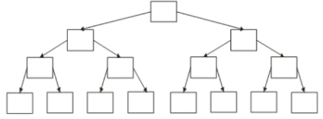
To the illustration of developing effective parallel algorithm and the way of its complexity evaluating we used applied problem of discrete fast Fourier Transform (DFFT). In relation to it we illustrate the principle of divide and conquer decomposition model (DM), which is used to decompose DFFT.
Figure 5. Illustration of divide and conquer DM (n=8).
4. The Role of Performance
Modeling techniques allow to model contention both at hardware and software levels by combining approximate solutions and analytical methods [30]. We would like to prefer analytical methods although the complexity of parallel computers and parallel algorithms could limit the applicability of these techniques. To the verification of analytical results we would like to use simulation method or in some cases experimental measuring.
4.1. Performance Evaluation Methods
To performance evaluation of parallel algorithms we can use analytical approach to get under given constraints analytical laws or some other derived analytical relations. We can use following solution methods to get a function of complex performance
• analytical
order (asymptotic) analysis [2, 12] Petri nets [4]
queuing theory [8, 14] • simulation [19]
• experimental
benchmarks [16] modeling tools [22] direct measuring [6, 27].
Analytical method is a very well developed set of techniques which can provide exact solutions very quickly, but only for a very restricted class of models. For more general models it is often possible to obtain approximate results significantly more quickly than when using simulation, although the accuracy of these results may be difficult to determine [31].
Simulation is the most general and versatile means of modeling systems for performance estimation. It has many uses, but its results are usually only approximations to the exact answer and the price of increased accuracy is much
longer execution times. They are still only applicable to a restricted class of models in spite of its computation and time requirements.
Evaluating system performance via experimental measurements is a very useful alternative for computer systems. Measurements can be gathered on existing systems by means of benchmark applications that aim at stressing specific aspects of computers systems. Even though benchmarks can be used in all types of performance studies, their main field of application is competitive procurement and performance assessment of existing parallel computers and parallel algorithms.
5. Performance Evaluation Criterions of
PA
To evaluations of parallel algorithms there have been developed several fundamental concepts. Tradeoffs among these performance factors are often encountered in real-life applications.
5.1. Basic Performance Concepts
5.1.1. Parallel Execution Time
We have defined parallel execution time T(s, p) as the execution time performed by p computing nodes (processors, cores, workstations) of given parallel computer and s defines input size (load) of given problem. Then T(s, 1) defines execution time for classic sequential computer.
5.1.2. Speed Up
The speed up factor S(s, p) we can define as
) , (
) 1 , ( ) , (
p s T
s T p s
S =
Speed up factor (dimensionless) is a measure obtained at given complex algorithm using p computing nodes solving given problem with its problem size s. Since S(s, p) ≤ p, we would like to design algorithms that achieve S(s, p) ≈ p.
5.1.3. Efficiency
The efficiency for processor system with p computing nodes is defined by
) , (
) 1 , ( ) , ( ) , (
p s T p
s T
p p s S p s
E = =
The efficiency is always less than 1. A value of E(s, p) approximately equal to 1 for given p, indicates that such parallel computer, using p computing nodes runs approximately p times faster than it does on sequential computer.
5.1.4. The Isoefficiency Concept
which is needed to achieve given fixed efficiency E (s, p). Let h(s, p) be the total overhead function consisted from existed overhead latencies involved in PA implementations. This overhead function is a function of both parallel computer size p and input problem size s. Then we can define efficiency E(s, p) of a parallel algorithm as
) , ( ) (
) ( )
, (
p s h s w
s w p
s E
+ =
The workload w(s) corresponds to useful performed parallel computations while the overhead function h(s, p) represents latency times attributed to communication of parallel processes, synchronization, waiting to shared resources etc. In general, the overheads increase with respect to increasing both values of parameters p and s. The question is hinged on relative growth rates between w(s) and h(s, p). With a fixed problem size the efficiency E(s, p) decreases as p increase. The reason is that the overhead function h(s, p) increases with p. With a fixed parallel computer size, the overhead function h(s, p) grows slower than the workload w(s). Thus the efficiency E(s, p) increases with increasing problem size s for a fixed parallel computer size. Therefore, one can expect to maintain a constant efficiency E(s, p) if the workload w(s) is allowed to grow properly with increasing parallel computer size p.
5.2. Complex Performance Modeling of PA
Complex performance modeling of PA we qualify as modeling with considering overhead function h(s, p) in all defined fundamental performance concepts T(s, p), S(s, p), E(s, p) and w(s).
5.2.1. Complex Parallel Execution Time
Complex parallel execution time T(s, p)complex will be
defined as the whole parallel execution time included overhead function h(s, p) as follows
p) h(s, ) , ( )
,
(s p =T s p +
T complex
5.2.2. Complex Speed Up Factor
The complex speed S(s, p)complex we can rewrite as
complex complex
p s T
s T p
s S
) , (
) 1 , ( )
,
( =
5.2.3. Complex Efficiency
Similarly the complex efficiency E(s, p)complex we can
rewrite as
complex complex
complex
p s T p
s T p
p s S p
s E
) , (
) 1 , ( )
, ( )
,
( = =
5.2.4. Isoefficiency Function
We rewrite equation for efficiency concept E(s, p) as E(s, p) = 1/(1 - h(s, p) / w(s). In order to maintain a constant E(s, p), the workload w(s) should grow in proportion to the overhead h(s, p). This leads to the following relation
) , ( ) , ( 1
) , ( )
( h s p
p s E
p s E s w
− =
The factor C = E(s, p)/1 - E(s, p) is for a given efficiency E(s, p) constant. We can then define the isoefficiency function as follows
) , ( )
(s C h s p
w =
5.2.5. Overhead Function
Overhead function h (s, p) defines coincident overhead latencies of given PA (shared memory, distributed memory, hybrid).The typical existed overheads of PA are as follows
• communication latency T(s, p)comm
• parallelization latency T(s, p)par
• synchronization latency T(s, p)syn
• waiting latency to use shared resource T(s, p)wait
• influence of parallel computer architecture T(s, p)arch
• specific latency of given PA T(s, p)spec.
Taking into account all named overhead latencies the overhead function h(s, p) is as follows
(
)
∑
= Ts pcomm T s ppar Ts psyn T s parch T s pspec
p s
h(, ) (, ) , (, ) , (, ) , (, ) , (, )
and the complex parallel execution time will be defined as follows
) , ( )
, ( )
,
(s p T s p h s p
T complex = comp +
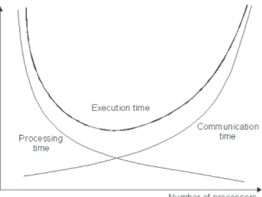
In general influence of at least most important overhead latencies is necessary to take into account in performance modeling of parallel algorithms because their influence to complex parallel execution time T(s, p)complex could be
dominant. The illustration of such dominant influence of communication overhead latency T(s, p)comm to own
parallel computation time T(s, p)comp is shown at Figure 6.
Figure 6. Illustration of dominant influence of T(s, p)comm to T(s, p)comp.
5.2.6. Modeling of PA Latencies
5.2.6.1. Own Parallel Computation Time
Own computation time T (s, p)comp of PA is given
through quotient of maximal time of running parallel processes i. e. as product of complexity Cpp (complexity of
maximal parallel process) and a parameter tc as an average
block of instructions etc.) divided by number of used computing nodes p of used parallel computer. Parallel computation execution time T(s, p)comp is then given as
follows
. )
p , (
p t C s
T comp = pp c
In general execution time of sequential and parallel algorithms are given through multiplicity product of algorithm complexity Calg (dimensionless number of
considered computation units) and a parameter tc as an
average value of performed considered operations (instructions, computing steps etc.).
For asymptotic complexity of parallel execution time T(s, p)comp supposing well paralleled problems is then given as
0 . lim
) p ,
( = →∞ =
p t C s
T comp p pp c
5.2.6.2. Modeling of Overhead Latencies
Overhead latencies are defined with its overhead function h(s, p). For every concrete parallel algorithm (shared memory, distributed memory, hybrid), or a similar group of PA, we are able to define their overhead function h(s, p) considering at least the most important overhead latencies of given PA. The individual latencies of given PA comes out from used decomposition model. Complex modeling based on considering overhead function h(s, p) of given PA opens unified complex modeling of any developed parallel algorithm.
5.2.6.2.1. Modeling of Communication Latency
Inter process communication of parallel processes (IPC) T(s, p)comm (communication latency) influences in a
decisive degree used decomposition model of PA. Obviously it is higher in distributed computing than in parallel one. For example world known parallel computing model with shared memory PRAM (Parallel Random Access Machine) does not consider communication latency. To model communication latency we have applied theory of complexity to inter process communication of parallel processes in a similar way as in modeling computation latency focusing to a number of performed communication steps (communication complexity). Then communication latency T(s, p)comm is given through number of performed
communication steps (communication complexity) for used decomposition model of given PA. Every communication step within parallel computer based on NOW module we can characterized through two basic communication parameters as follows
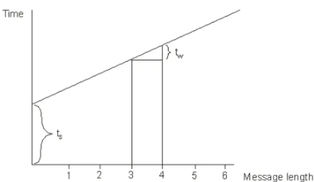
• communication parameter ts defined as parameter for
initialization of communication step (start up time) • communication parameter tw as parameter for
transmission latency of considered data unit (typically word).
Illustration of defined communication parameters is at Figure 7. These communication parameters ts, tw are
constants for concrete parallel computer [10].
The whole communication overhead latency is given through two basic following functions
• function f1(ts) which represents the whole number of
communication initializations for given parallel process
• function f2(tw) which correspondents to whole
performed data unit transmission (usually time of word transmission for given parallel computer) in given parallel process.
Figure 7. Illustration of communication parameters.
These two defined functions limit performance of used parallel computer on defined NOW module of parallel computer. Then using a superposition we can write for communication latency in NOW module T(s, p)comm as
follows
) ( ) ( )
,
(s p commNOW f1 ts f2 tw
T = +
To the practical illustration of communication overheads we used discrete fast Fourier transform (DFFT) representing typical matrix parallel algorithm with divide and conquer decomposition model.
To derive the whole communication latency T(s, p)comm
in other dominant parallel computers based on integration of NOW modules (network of NOW modules named as Grid) we need to extend the considered two communication functions f1(ts), f2(tw) in NOW module by third function
component f3(th), which will determine potential multiple
crossing used NOW modules of integrated parallel computer. This third function is characterized through multiplying hops parameter lh among NOW modules
(generally NOW networks) and average communication latency time of jumped NOW modules with the same communication speed or a sum of individual communication latencies for jumped NOW modules with their different communication speed. Then in general to the whole communication latency in Grid is valid
∑
=
+
+
=
ui
h w s w
s
commGRID
f
t
f
t
f
t
t
l
p
s
T
1 3 2
1
(
)
(
)
(
,
,
)
)
,
(
In general communication latency time f3(ts, tw, lh) is
lh hops. The communication time for one communication
step is then given as ts+ m twlhth, where the new parameters
are.
• lh is the number of network hops
• m is the number of transmitted data units (usually words)
• th is average communication time for one hop.
The new communication parameters th, lh depend from a
concrete architecture of Grid communication network and used routing algorithm. In [11] we have developed unified models which could help to establish these parameters for dominant parallel computers. For the complex analytical modeling there is necessary to derive for given parallel algorithm or a group of similar algorithms (matrix parallel algorithms) needed communication functions and that always individually for any decomposition strategy) isoefficiency function and defined technical parameters (computational, communication) for used parallel computer (NOW, Grid).
5.2.6.2.2. Modeling of Parallelization Latency
The parallelization latency T(s, p)par represents overhead
latency of PA though parallelization of given complex problem. Its consequences are mostly projected as additional communication complexity to T(s, p)comm.
5.2.6.2.3. Modeling of Synchronization Latency
The third part of h(s, p) function T(s, p)syn we can
eliminate through optimization of load balancing among individual computing nodes of used parallel computer. For this purpose we would measure performance of used computing nodes for given developed parallel algorithm and then based on these achieved results we are able to redistribute better workload of computing nodes. This activity we can repeat until we have optimal redistributed input load (optimal load redistribution based on real performance results).
5.2.6.2.4. Modeling of Influence of Parallel Computer Architecture
The fourth part of h(s, p) overhead function T(s, p)arch
(influence of parallel computer architecture) we will model with defined technical parameters tc, ts, tw, which are
constant for given parallel computer [10].
5.2.6.2.5. Modeling of Waiting Latency
The fifth part of h(s, p) overhead function T(s, p)wait
represents whole waiting times to use shared resources of parallel computer (memory modules, communication channels, I/O devices etc.). This kind of overhead latency is typical in using shared technical resources in a massive way (shared memory modules, communication channels, I/O devices etc.). We can only limit it by optimal allocation of shared resources. To model this overhead latency in an analytical way is a very crucial problem. We have been modeling it in an analytical way applied queuing theory results in combination with experimental measurements [10, 11].
5.2.6.2.6. Modeling of Specified PA Latency
The sixth part of h(s, p) overhead function T(s, p)spec
(influence of specified PA) represents any other possible specific overhead latency of given parallel algorithm.
5.2.6.3. Asymptotic Analytical Modeling of PA
Most of to this time known results in analytical modeling of PA in the world for extended classical parallel computers with shared memory (supercomputers, SMP and SIMD systems) or parallel computers with distributed memory based on some cluster of computing nodes mostly did not consider existed overhead influences of PA supposing that they are lower in comparison to the own computation latency T(s, p)comp of performed computations . In this
sense analysis and modeling of complexity in parallel algorithms (PA) were rationalized to the analysis of only computation complexity of PA, that mean that the defined function of control and communication overheads h(s, p) were not a part of derived relations for the whole parallel execution time.
The complexity function in the relation for isoefficiency supposed, that dominate influence to the whole complexity of PA has computation complexity of performed massive computations. Such assumption has been proved to be true mainly in using classical parallel computers in the world (supercomputers, massive SMP – shared memory, SIMD architectures etc.). To map mentioned assumption to the relation for asymptotic isoefficiency w(s) means that
[
Tspcomp h sp Tspcomp]
[
Tspcomp]
s
w()=max (, ) , (, )< (, ) =max (, )
But in our unified complex modeling of PA possible influence of any part of defined overhead function h(s, p) could be dominant in a nonlinear way. Then for complex isoefficiency function it is necessary to consider it as follows
[
( , ) , ( , )]
max)
(s T s p h s p
w = comp
6. Discrete Fourier Transform
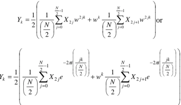
The discrete Fourier transform (DFT) has played an important role in the evolution of digital signal processing techniques. It has opened new signal processing techniques in the frequency domain, which are not easily realizable in the analogue domain. The DFT is a linear transformation that maps n regularly sampled points from a cycle of a periodic signal, like a sine wave, onto an equal number of points representing the frequency spectrum of the signal. The discrete Fourier transform (DFT) is defined as [3, 7]
∑
−=
−
=
1
0 2 1 N
j
N jk i
j
k X e
N Y
π
∑
− = =
1 0 2 N j N jk i jk
Y
e
X
π
for 0 ≤ k ≤ N-1. For N real input values X0, X1, X2, …, XN-1,
transforms generates N complex values Y0, Y1, Y2, …, YN-1.
If we use
w
=
e
−2πi/N , that is w is N–th root of complex number i in complex plane we get∑
− ==
1 01
N j jk jk
X
w
N
Y
and in inverse as
∑
− = −=
1 0 N j jk jk
Y
w
X
Variable w is a basic part of DFFT computations and is named as twiddle factor. Defined transformation equations are on principle linear transformations.
A direct computation of the DFT or the IDFT requires N2 complex arithmetic operations. For example the time required for just the complex multiplication in a 1024point DFT is Tmult=1024 . 4. Treal, where we assumed that one
complex multiplication corresponds to four real multiplications and the time required for one real multiplication (Treal) is known for given computer. But with
this approach we could take into account only the computation times and not also the overheads delays connected with implantation on parallel way.
6.1. The Discrete Fast Fourier Transform
DFFT is a fast method of DFT computation with time complexity O (N / 2 log2(N)) in comparison to sequential
DFT algorithm complexity as O(N2). For a quick computation of the DFT is used adjustment of Cooley-Tukey [7]. To come to final adjustment we start with a modified form of the DFT.
∑
− ==
1 01
N j jk jk
X
w
N
Y
In general demanded sum is divided to two parts using decomposition strategy “divide-and-conquer”. Its principle we describe with modification of origin sum to two following pairs as
+ =
∑
∑
− = + + − = 1 2 0 ) 1 2 ( 1 2 1 2 0 2 2 1 N j k j j N j jk jk X w X w
N
Y ,
where the first part of sum contents result part with even indexes and second part with odd indexes. In this sense we get + =
∑
∑
− = + − = 1 2 0 2 1 2 1 2 0 2 2 2 1 2 1 2 1 N j jk j N j k jk jk X w
N w w X N Y or + =
∑
∑
− = − + − = − 1 2 0 2 2 1 2 1 2 0 2 2 2 2 1 2 1 2 1 N j N jk i j N j k N jk i jk X e
N w e X N Y π π
Every part of sum means DFT on N/2 values with even indexes and N/2 values with odd indexes. Then we can
formally write
(
)
odd k even
k Y w Y
Y = +
2
1 for k=0, 1, 2, ....,
N-1, whereby Yeven is N/2 – point DFT on the values with
even indexes X0, X2, X4, … and Yodd is N/2 – point
transformation on values X1, X3, X5, ….Supposed that k is
limited to first 0, 1, …, N/2–1, N/2 values from whole number of N values. The whole series we can divide to two following parts
(
odd)
k even
k Y wY
Y = +
2 1
and
(
odd)
k even odd N k even N k Y w Y Y w Y
Y = −
+ = + + 2 1 2 1 2 2 ,
because wk+N/2 = - wk, where 0 0 ≤ k < N/2. In this way we can compute Yk and Yk+N/2 in a parallel way using two N/2
– point transformations according illustration at Figure 8. Every from N/2 – point DFT we can again divide to next parts, that is to two N/4 – point DFT. Applied decomposition strategy could follows till to exhausting dividing possibility for given N. Dividing factor is named as radix - q, and that for dividing number higher than two.
Figure 8. Divide and conquer decomposition strategy for DFFT.
significant for large N. Direct calculation of the DFT or IDFT, according to the following program requires N2 complex arithmetic operations.
Program Direct_DFT; var
x, Y: array[0..Nminus1] of complex; begin
for k:=0 to N-1 do begin
Y[k] :=x[0]; for n:=1 to N-1 do
Y[k] := Y[k] + Wnk * x[n]; end;
end.
The difference in execution time between a direct computation of the DFT and the new DFFT algorithm is very high for large N. For example the time required for the complex multiplication in a 1024-point FFT is Tmult = 0,5 .
N .log2(N) . 4 .Treal = 0,5 . 1024 .log2(1024) . 4 .Treal, where
the complex multiplication corresponds approximately to four real multiplications.
6.2. Parallel Algorithms of Discrete Fast Fourier Transform
Cooley and Tukey have developed the fast DFFT algorithm which requires only O(N.log2(N)) operations.
The difference in execution time between a direct computation of the DFT and the new DFFT algorithm is very large for large N. For example the time required for just the complex multiplication in a 1024-point FFT is Tmult= 0,5.N log2(N).4.Treal = 0,5.1024. log2(1024).4. Treal,
where the complex multiplication corresponds approximately to four real multiplications. The basic form of parallel DFFT is the one-dimensional (1-D), unordered and radix–2 algorithms (using divide and conquer strategy according the principle at Figure 9). The effective parallel computing of DFFT tends to computing one dimensional DFFT with radix greater than two and computing multidimensional FFT by using the polynomial transfer methods. In general a radix-q DFFT is computed by splitting the input sequence of size s into a q sequences of size n/q each, computing faster the q smaller DFFT, and then combining the result. For example, in a radix-4 FFT, each step computes four outputs from four inputs, and the total number of iterations is log4 s rather than log2 s. The
input length should, of course, be a power of four. Parallel formulations of higher radix strategies (radix-3, radix-5) 1-D or multidimensional DFFT are similar to the basic form because the underlying ideas behind all sequential DFFT are the same [32]. An ordered DFFT is obtained by performing bit reversal (permutation) on the output sequence of an unordered DFFT. Bit reversal does not affect the overall complexity of a parallel implementation.
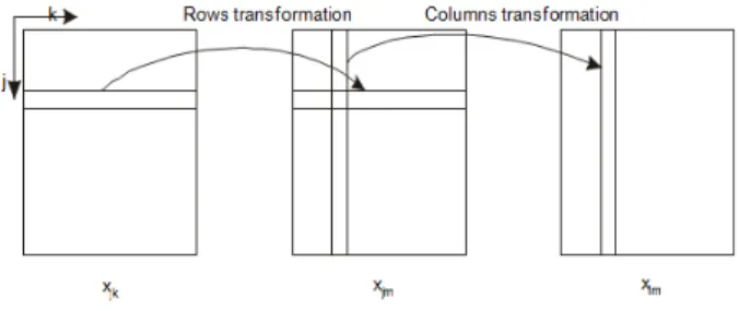
6.3. Two-Dimensional 2D DFFT
Processing of images and signals often requires the
implementation of a multi-dimensional discrete fast Fourier transform (DFFT).Simplest method of computation of two dimensional DFFT (2D DFFT)is computation of one dimensional DFFT (1D DFFT) on each row and then follows computation of one dimensional DFFT for each column. This illustrates Figure 9.
Figure 9. Two dimensional DFFT.
6.4. Analyzed Examples
6.4.1. One Element per Processor
This is the simplest example of complexity evaluation of the DFFT. In this case we consider a p=s parallel processor (d-dimensional hypercube architecture) to compute s-point DFFT. A hypercube is a multidimensional mesh of processors with exactly two processors in each dimension. A d-dimensional hypercube consists of p=2d processors. In a d-dimensional hypercube each processor is directly connected to d other processors. In this case we can simply derive that T(s, 1) = s log s and T(s, p) = log s. Then speedup factor S(s, p) = p and system efficiency E(s, p) = 1. Such a formulation of DFFT algorithm for a d-dimensional hypercube calculation is cost optimal but for the higher values of s and use of p=s processors could be only hypothetical.
6.4.2. Multiple Elements per Processor
This is very real case of practical DFFT parallel computations. In this example we examine implementing the binary exchange algorithm to compute an s-point DFFT on a hypercube with p processors, where p > s. Assume that both s and p are powers of two. According the Figure 10, we partition the sequences into blocks of s/p contiguous elements and assign one block to each processor. Assume that the hypercube is d-dimensional (p=2d) and s=2r. Figure 10 shows that elements with indices differing in their d (=2) most significant bits e mapped onto different processors. However, all elements with indices having the same r-d most significant bits are mapped onto the same processor. Hence, this parallel DFFT algorithm performs inter process communication only during the first d = log p of the log s iterations. There is no communication during the rested r – d iterations.
Each communication operation exchanges s/p words of data. Since all communications takes place between directly-connected processors, the total communication time does not depend on the type of routing. Thus the time spent in communication in the DFFT algorithm is ts log p +
the per-word transfer time. These times are known for the concrete parallel system. If a complex multiplication and addition pair takes time tc, then the parallel run time for
s-point DFFT on a p-processor hypercube is as follows
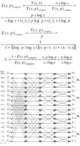
p p s t p t s p s t p s
T( , )complex = c log + slog + w log
The expressions for complex speedup S(s, p)complex,
efficiency E(s, p)complex and defined constant C (part of
issoefficiency function) are given by the following equations p s t t p p t t s s s s p p s T s s t p s T s T p s S c w c s complex c complex complex log ) / ( log ) / ( log log ) , ( log ) , ( ) 1 , ( ) , ( + + = = = =
[
]
{
(log /log ) ( / ) ( / )}
1 1 ) , ( ) , ( w c c s complex complex t t s t p t s p p p s S p s E + + = = = s t p t s s t p p t p s E p s E C c w c s complex complex log log log log ) , ( ) , ( 1 + = − =Figure 10. 16-point DFFT on four processors.
6.4.3. Multiple Elements per Processor with Routing
This is a most complicated, but very real, case in parallel computing. It is typical for the parallel architectures, in which the processors do not have enough direct connected processor to compute the given parallel algorithm. Then the communication of not direct connected processors or computers is realized through a number (hop) of other processors or communication switches according some routing algorithm.
The time for sending a message of size m between processors, that are lh hops apart is given by ts,+ thlh where
ts is the starting message time and th is the overhead time
for one hop. The values ts, th, lh depend from the
architecture of parallel system (mainly its interconnection
network) and routing strategy. If we can define these values for a concrete parallel system and routing strategy, cost performance tradeoffs are to be analyzed in a similar way than in previous case.
6.4.3. Multiple Elements per Processor in NOW
An example of our experimental parallel computer based on NOW we have illustrated at Figure 2. Based on this used NOW module communication overheads depends on topology of communication network and its communication parameters (transmission speed, bandwidth, transmission control etc.). To verify derived analytical results we have performed some simulation experiments in NOW module with DFFT’s PA. From performed experiments comes out that for effective parallel computing of DFFT the use of centralized massively parallel system should by preferred to asynchronous parallel computers based on NOW modules. At experimental testing we have used workstations of NOW parallel computer as follows
• WS 1 – Pentium IV (f = 2.26 GHz)
• WS 2 - Pentium IV Xeon (2 proc., f = 2.2 GHz) • WS 3 - Intel Core 2 Duo T 7400 (2 cores, f=2.16
GHz)
• WS 4 - Intel Core 2 Quad (4 cores, f = 2.5 GHz) • WS 5 - Intel SandyBridge i5 2500S (4 cores, f=2.7
GHz).
7. Results
As scalable parallel computer we have defined any parallel computer in which the efficiency can be kept fixed as the number of computing nodes is increased, provided that the problem size is also increased. The scalability of a PA/parallel computer combination determines its capacity to use an increased number of computing nodes p effectively. We have considered the Cooley-Tukey algorithm for one dimensional s-point DFFT to maintain the same efficiency. Figure 11 illustrates the efficiency E(s,
p)complex of the binary exchange DFFT parallel algorithm as
a function of s on a 512 processors (computing nodes) hypercube parallel computer with its following technical parameters tc=2µs, tw= 4 µ s and ts =25 µs. The threshold
point is given as tc / (tc + tw) = 0,33. The efficiency initially
increases rapidly with the problem size to the threshold, but then the efficiency curve platens out beyond the threshold. The binary exchange algorithm yields good performance on a hypercube provided that the communication bandwidth and the processing speed of the computing nodes are balanced. Efficiencies below a certain threshold can be maintained while increasing the problem size at a moderate rate with an increasing number of processors. We can say that the use of transpose algorithm will have much higher overhead than the binary exchange algorithm due to message start up time ts, but has a lower overhead due to
per-word transfer time tw. As a result, either of the two
other architectures with common memory have ts very low
in comparison to typical NOW or Grid.
Figure 11. The efficiency E(s, p)complex of the DFFT binary exchange parallel algorithm.
However, this threshold is very low if the communication bandwidth of the hypercube is low, compared to the speed of its processors. Therefore it is necessary to describe a different parallel formulation of DFFT for interconnection network of computer network. Such a formulation involves matrix transposition for an array of s-input points and hence we called it the transpose parallel algorithm. In principal we can say that the use of transpose PA will have a much higher overhead than the binary exchange algorithm due to message start up time ts,
but has a lower overhead due to per-word transfer time tw.
As a result, either of the two algorithm formulations may be faster depending on the relative values of ts and tw. In
principle parallel computers with shared memory have ts
very low in comparison to typical dominant parallel computers based on NOW and Grid.
The influence of matrix dimension for DFFT to the communication overheads in computer network of personal computers is illustrated at the Figure 12. From this picture we can see that to more effective DFFT computing in computer network there is necessary another transpose algorithm.
Figure 12. The influence of the network load on the matrix dimension.
The performance results in parallel computer NOW based on Ethernet we have graphically illustrated for 2D FFT at the Figure 13. These results of 2D FFT parallel algorithm document increasing of both computation and communication parts in geometrically way with the quotient value nearly four for analyzed matrix dimensions and that in increasing matrix dimension mean to do twice more computation on columns and twice more on rows.
Figure 13. Results in NOW for T(s, p)complex of 2DFFT for Ethernet.
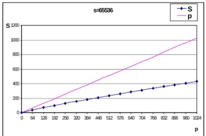
At Figure 14 we have illustrated parallel speed up S(s, p)complex of 1D DFFT parallel algorithm with binary data
exchange for defined workload s = 65 536 (s=n2 / p) as function of number of computing nodes p. Character of S(s, p)complex is sub linear i. e. always less as illustrated p curve
(ideal speed up without overheads) as a consequence of overhead latencies (architecture, communication, synchronization etc.) of used parallel computer.
Figure 14. Illustration of S (s, p)complex as factor of computing nodes number p.
Figure 15 illustrates isoefficiency functions w(s)complex of
1D DFFT parallel algorithm. For lower values of E(s, p) (0,1; 0,2; 0,3; 0,4; 0,45) to the threshold (E = 0,33) we have used based on performed analysis in theoretical part computed using following expression
0 0.05 0.1 0.15 0.2 0.25 0.3 0.35 0.4 0.45 0.5
0 5000 10000 15000 20000 25000 30000 35000 s E
Treshold
0 5000 10000 15000 20000 25000 30000 35000 40000
Execution time [ms]
Network nodes
64x64 128x128 256x256 512x512 1024x1024
64x64 327 150 141 133
128x128 1067 527 452 415
256x256 5759 2924 2912 2891
512x512 17215 8667 8624 8614
1024x1024 68841 34051 33931 33768
WS1 WS3 WS4 WS5
s=65536
0 200 400 600 800 1000 1200
0 64 128 192 256 320 384 448 512 576 640 704 768 832 896 960 1024 p S
p p t t C s s s
w
c s
complex log log
)
( = =
and the values above the threshold of efficiency function were computed on following relation
p p
t t C s
w Ctwtc
c w
complex log
)
( = /
Figure 15. Issoefficiency function w(s)complex of 1D DFFT (E =0,1; 0,2; 0,3; 0,4; 0,45).
Figure 16 illustrates issoefficiency functions w(s)complex
1D DFFT on hypercube parallel computer for the values of E(s, p)complex = 0,5 and E(s, p)complex =0,55. From illustrated
curves at Figure 18 we can see in theoretical part of this section predicted stormy growth of issoeficiency function w(s)complex i.e stormy tendency of algorithm scalability for
analyzed parallel algorithm 1D DFFT with binary data exchange past the threshold.
Figure 16. Issoefficiency function w(s)complex of 1D DFFT (E =0,5; 0,55).
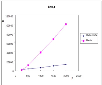
Figure 17 illustrates influence of parallel computer architecture to its algorithm scalability based on given efficiency for E(s, p)complex = 0,4 according the derived
conclusions in theoretical part of this section. We
considered the Cooley-Tukey algorithm for one dimensional s-point DFFT parallel algorithm with binary data exchange. We can see that this parallel algorithm is essentially better scalable for the hypercube parallel architecture as for the mesh parallel computer. This implies better architecture of communication network in hypercube for parallel solution of 1D DFFT with binary data exchange (lover communication latency). This verified resulting idea documents important role of parallel computer architecture to the whole performance of given parallel algorithm. The scalability of an algorithm-architecture combination determines its capacity to use effectively an increased number of computing nodes p.
Figure 17. Influence of parallel computer architecture to scalability.
8. Conclusions
Performance evaluation as a discipline has repeatedly proved to be critical for design and successful use of parallel computers and parallel algorithms too. At the early stage of design, performance models can be used to project the system scalability and evaluate design alternatives. At the production stage, performance evaluation methodologies can be used to detect bottlenecks and subsequently suggests ways to alleviate them. Analytical methods (order analysis, queuing theory systems and Petri nets), simulation, experimental measurements, and hybrid modeling methods have been successfully used for the evaluation of system and its components too. Via the extended form of complex isoefficiency concept we have illustrated its concrete using to predicate the performance in applied matrix parallel algorithms.
To derive complex isoefficiency function in analytical way it is necessary to derive al typical used criterion for performance evaluation of parallel algorithms including their overhead function h(s, p). Based on these relations we are able to derive complex issoefficiency function as real criterion to evaluate and predict performance of parallel algorithms also for theoretical (not existed) parallel computers. So in this way we can say that this process includes complex performance evaluation including
0 10000 20000 30000 40000 50000 60000 70000
0
100 200 300 400 500 600 700 800 900100011001200 130014001500
p W
E=0,1
E=0,2
E=0,3
E=0,4
E=0,45
0,00E+00 5,00E+07 1,00E+08 1,50E+08 2,00E+08 2,50E+08 3,00E+08
0
100 200 300 400 500 600 700 800 900100011001200130014001500
p W
performance prediction.
This paper continues in applying complex analytical modeling to another group of matrix parallel algorithms (MPA) which is characterized by decreasing number of decomposed matrix elements (decreasing of complexity) in process of parallel execution. To present this group of MPA we have chosen discrete fast Fourier transform (DFFT) as Pa with its intensive communication complexity. On various real examples of the DFFT we have described complexity determination of PA not only for illustrated DFFT PA but also for other similar MPA. The considered complex analyzed examples we have been evaluated so on classic massive parallel computers (hypercube, mesh) as on actually dominant parallel computers NOW and Grid. It is obvious that in some cases using of network of workstations (NOW) or its higher integration parallel computers named as Grid (integrated network of NOW networks) could be less effective than on innovated classic massive parallel computers but NOW and Grid belong to more flexible and perspective parallel computers.
Acknowledgements
This work was done within the project “Modeling, optimization and prediction of parallel computers and algorithms” at University of Zilina, Slovakia. The author gratefully acknowledges help of project supervisor Prof. Ing. Ivan Hanuliak, PhD.
References
[1] Abderazek A. B., Multicore systems on chip - Practical Software/Hardware design, Imperial college press, pp. 200, 2010
[2] Arora S., Barak B., Computational complexity - A modern Approach, Cambridge University Press, pp. 573, 2009 [3] Casanova H., Legrand A., Robert Y., Parallel algorithms,
CRC Press, 2008
[4] Desel J., Esperza J., Free Choise Petri Nets, Cambridge University Press, UK, pp. 256, 2005
[5] Dubois M., Annavaram M., Stenstrom P., Parallel Computer Organization and Design, pp. 560, 2012
[6] Dubhash D.P., Panconesi A., Concentration of measure for the analysis of randomized algorithms, Cambridge University Press, UK, 2009
[7] Edmonds J., How to think about algorithms, Cambridge University Press, UK, pp. 472, 2010
[8] Gelenbe E., Analysis and synthesis of computer systems, Imperial College Press, pp. 324, 2010
[9] Hager G., Wellein G., Introduction to High Performance Computing for Scientists and Engineers, pp. 356, July 2010 [10] Hanuliak P., Analytical method of performance prediction in
parallel algorithms, The Open Cybernetics and Systemics Journal, Vol. 6, Bentham, UK, pp. 38-47, 2012
[11] Hanuliak M., Unified analytical models of parallel and distributed computing, American J. of Networks and Communication, Science PG, Vol. 3, No. 1, USA, pp. 1-12, 2014
[12] Hanuliak M., Hanuliak I., To the correction of analytical models for computer based communication systems, Kybernetes, Vol. 35, No. 9, UK, pp. 1492-1504, 2006 [13] Hanuliak M., Performance modeling of Nov and Grid
parallel computers, AD ALTA – Vol. 3, issue 2, Hradec Kralove, Czech republic, pp. 91-96, 2013
[14] Harchol-BalterMor, Performance modeling and design of computer systems, Cambridge University Press, UK, pp. 576, 2013
[15] Hwang K. and coll., Distributed and Parallel Computing, Morgan Kaufmann, pp. 472, 2011
[16] John L. K., Eeckhout L., Performance evaluation and benchmarking, CRC Press, 2005
[17] Kshemkalyani A. D., Singhal M., Distributed Computing, University of Illinois, Cambridge University Press, UK, pp. 756, 2011
[18] Kirk D. B., Hwu W. W., Programming massively parallel processors, Morgan Kaufmann, pp. 280, 2010
[19] Kostin A., Ilushechkina L., Modeling and simulation of distributed systems, Imperial College Press, pp. 440, 2010 [20] Kumar A., Manjunath D., Kuri J., Communication
Networking , Morgan Kaufmann, pp. 750, 2004
[21] Kushilevitz E., Nissan N., Communication Complexity, Cambridge University Press, UK, pp. 208, 2006
[22] Kwiatkowska M., Norman G., and Parker D., PRISM 4.0: Verification of Probabilistic Real-time Systems, In Proc. of 23rd CAV’11, Vol. 6806, Springer, pp. 585-591, 2011 [23] Le Boudec Jean-Yves, Performance evaluation of computer
and communication systems, CRC Press, pp. 300, 2011 [24] McCabe J., D., Network analysis, architecture, and design
(3rd edition), Elsevier/ Morgan Kaufmann, pp. 496, 2010 [25] Meerschaert M., Mathematical modeling (4-th edition),
Elsevier, pp. 384, 2013
[26] Misra Ch. S.,Woungang I., Selected topics in communication network and distributed systems, Imperial college press, pp. 808, 2010
[27] Miller S., Probability and Random Processes, 2nd edition, Academic Press, Elsevier Science, pp. 552, 2012
[28] Peterson L. L., Davie B. C., Computer networks – a system approach, Morgan Kaufmann, pp. 920, 2011
[29] Resch M. M., Supercomputers in Grids, Int. J. of Grid and HPC, No.1, pp. 1-9, 2009
[30] Riano l., McGinity T.M., Quantifying the role of complexity in a system´s performance, Evolving Systems, Springer Verlag, pp. 189–198, 2011
[32] Takahashi D., Kanada Y.: High-performance radix-2, 3 and 5 parallel 1-D complex FFT algorithms for distributed-memory parallel computers, J. of Supercomputing, 15, Kluwer Academic Publishers, The Netherlands, pp. 207-228, 2000
[33] Wang L., Jie Wei., Chen J., Grid Computing: Infrastructure, Service, and Application, CRC Press, 2009 www pages