Practical surface light fields

(1)

PRACTICAL SURFACE LIGHT FIELDS

Greg Coombe

A dissertation submitted to the faculty of the University of North Carolina at Chapel Hill in partial fulfillment of the requirements for the degree of Doctor of Philosophy in the Department of Computer Science.

Chapel Hill 2007

Approved by:

Anselmo Lastra

Radek Grzeszczuk

Leonard McMillan

Marc Pollefeys

(2)

c

2007 Greg Coombe

(3)

ABSTRACT

GREG COOMBE: Practical Surface Light Fields (Under the direction of Anselmo Lastra)

The rendering of photorealistic surface appearance is one of the main challenges

facing modern computer graphics. Image-based approaches have become increasingly

important because they can capture the appearance of a wide variety of physical surfaces

with complex reflectance behavior. In this dissertation, I focus on Surface Light Fields,

an image-based representation of view-dependent and spatially-varying appearance.

Constructing a Surface Light Field can be a time-consuming and tedious process.

The data sizes are quite large, often requiring multiple gigabytes to represent complex

reflectance properties. The result can only be viewed after a lengthy post-process is

complete, so it can be difficult to determine when the light field is sufficiently sampled.

Often, uncertainty about the sampling density leads users to capture many more images

than necessary in order to guarantee adequate coverage.

To address these problems, I present several approaches to simplify the capture of

Surface Light Fields. The first is a “human-in-the-loop” interactive feedback system

based on the Online SVD. As each image is captured, it is incorporated into the

repre-sentation in a streaming fashion and displayed to the user. In this way, the user receives

direct feedback about the capture process, and can use this feedback to improve the

sampling. To avoid the problems of discretization and resampling, I used Incremental

Weighted Least Squares, a subset of Radial Basis Function which allows for

incremen-tal local construction and fast rendering on graphics hardware. Lastly, I address the

limitation of fixed lighting by describing a system that captures the Surface Light Field

(4)

ACKNOWLEDGMENTS

Just as there is an African proverb that states “It takes a village to raise a child,” there should be an Academic proverb that states “It takes a big department to create a dissertation.” I am extremely lucky to have spent some of the best years of my life with the people of the University of North Carolina Computer Science Department. The people that I met through my time at UNC helped in numerous ways, which they may or may not know of, and which I will never be able to repay.

Most importantly, I would like to thank my advisor Anselmo Lastra, who has been a great inspiration to me both academically and personally. It is his ability to spot interesting research ideas (and discard unfruitful ones) that led me down the fruitful research path of this dissertation. I’d also like to thank him for being willing to help out when I was inevitably working at 4am the night before the paper deadline.

During a summer internship at Intel I had the privilege of working with Radek Grzeszczuk, who encouraged me to look at GPU implementations of Surface Light Fields. This became the first component of this dissertation and lead to all of the subsequent research. This has become somewhat of a trend for Radek, who also sparked the research of Wei-Chao Chen and Karl Hillesland before me. Working with him also gave me valuable insight into the world of industry research.

I would also like to thank Fred Brooks, Mary Whitton, and the members of the EVE Group for providing a unique and nurturing scientific environment for the exchange of ideas. I gained a tremendous amount through discussions. Leonard McMillan and the students of the Data Driven Modeling course gave encouragement and critiques of the research that would eventually become the second component of this dissertation.

(5)

dramatically less enjoyable.

I’d like to thank Bruce Gooch, whom I met in my undergraduate studies at the University of Utah. He encouraged me to get into research by joining the Alpha 1 research group, thus starting me down the long path that lead to this dissertation. Thanks to my friends and co-authors Josh Steinhurst and Justin Hensley for numerous research discussions about graphics hardware and global illumination. For several years, not a day would pass without a discussion of an interesting problem or new research topic. If only I had enough time to work on all of them!

I’d like to thank Jan-Micheal Frahm for helping me with the third component of this dissertation, and in particular helping me track down all of the possible sources of error in the capture device, and then devising creative and novel ways to quantify this error. I’d also like to thank Mark Pollefeys, Leonard McMillan, Radek Grzeszczuk, and Gary Bishop, for help during the research proposal and oral exam.

I would also like to thank the superb staff of the Computer Science Department, especially Bil Hays, Tim Quigg, Janet Jones, and Sandra Neely, who work every day to make our lives as grad students easier. I’m grateful to NVIDIA for funding my graduate career through both their International Graduate Student Fellowship and an interesting and enjoyable summer internship.

(6)

(7)

LIST OF TABLES

4.1 RMS Error values from reconstructing a WLS approximation while vary-ing the center layout. The error was computed with a trainvary-ing set of 64 images and an evaluation set of 74 images. The disk is a slight improve-ment in terms of error compared to the grid, and it has a large benefit in terms of reducing the variance of the error. . . 67

(11)

LIST OF FIGURES

1.1 Left: Spiderman 2 by Sony Imageworks. Right: Matrix Reloaded by ESC Entertainment. The top row shows a few of the source images captured as a pprocess. The bottom row shows novel viewpoints re-constructed from the imagery. In order to animate the SLF in the Matrix Reloaded, the artists collected several sets of SLFs with different extreme facial expressions, and interpolated between them to generate the facial expressions used in the movie. . . 2

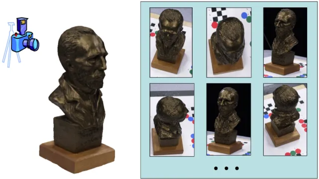
1.2 The first step in the SLF process is to capture a set of photographs of a real object from a variety of viewpoints. These images are processed to generate a compressed representation, which can be used to render novel images from this representation. Dataset courtesy of Intel Corp. . . . 3

1.3 A heart figurine, a marble pestle, and a copper pitcher captured and rendered with our online system. . . 6

1.4 A side-by-side comparison of the WLS reconstruction with an input im-age that was not included in the training set. . . 7

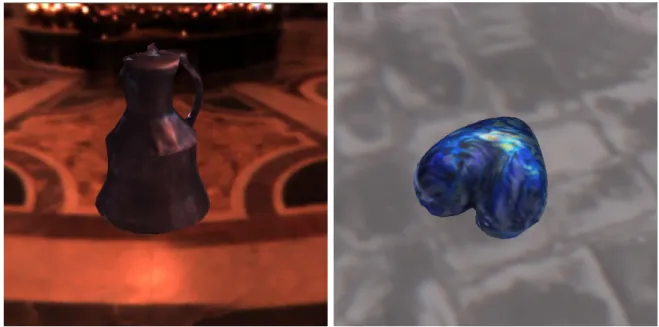
1.5 Left: pitcher model in St. Peter’s light probe. Right: heart model in Uffizi light probe. . . 8

2.1 The Bidirectional Subsurface Scattering Distribution Function. The in-cident light arrives at the surface point (ui, vi) from direction (θi, φi). It

is then scattered through the material and exits at surface point (ue, ve)

in direction (θe, φe). . . 12

2.2 A taxonomy of reflectance functions with dimensionality. From Mueller (Mueller et al., 2004). . . 13

2.3 Surface light fields can be represented as the function L(u, v, θ, φ), a 4D space composed of the product of the 2D space of surface points and the 2D space of view directions. . . 16

(12)

2.5 The surface functionsg(u, v) are parameterized across triangle rings. To get the color for the triangle, each of the three triangle ring functions are weighted byβ(u, v, k) and summed. The weighting function sums to 1.0 everywhere within the triangle. From Chen et al. (Chen et al., 2002). 19

2.6 Resampling of views. Left: The camera positions are projected onto the local basis. Center: Delaunay triangulation of views. Right: Resampling to uniform grid. From Chen et al. (Chen et al., 2002). . . 20

3.1 A heart figurine, a marble pestle, and a copper pitcher captured and rendered with our online system. . . 23

3.2 This sequence shows the image acquisition process. The left frame shows an image from the camera. In the middle is the reconstruction before this image is incorporated, with highlights interpolated from nearby views. The right image shows the reconstruction after it is incorporated, with the correct highlights. . . 25

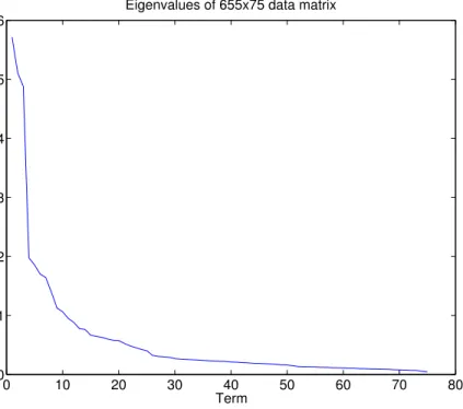
3.3 The eigenvalues of a 655x75 matrix from a SLF dataset. The mass of the eigenvalues are concentrated in the first dozen terms, which implies that a good approximation of the full matrix can be computed using only a subset of the eigenvectors and eigenvalues. . . 28

3.4 The Online SVD. A new point c is incorporated into the existing SVD. The orthogonal component p is computed by projecting onto U. If kpk

is below a threshold, then we can incorporate this new sample by simply rotating U. Otherwise, we must increase the rank of the approximation by adding another eigenvector that is orthogonal to the current set of eigenvectors. . . 31

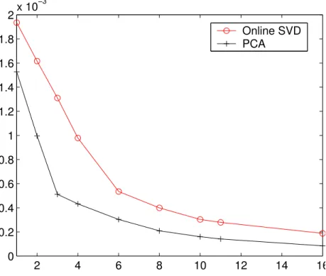
3.5 The Mean Squared Error of a reconstructed light field as a function of the rank. The majority of the light field is captured after 4-6 terms. For the same number of terms, the Online SVD has more error than the batch SVD. . . 33

(13)

3.7 The data-driven quality heuristicψ(s, t, θ, φ) displayed on the star model. Left: The heuristic is dark in areas where images have already been captured, indicating that the area has been well-sampled. Right: In areas where more data is needed, the heuristic is bright to draw attention to the area. . . 36

3.8 A side-by-side comparison of the Buddha model constructed with the OpenLF system (left) and our incremental approach (right). There are some slight differences noticeable in the chest area. . . 37

3.9 Acquiring the geometry of a marble pestle. Left: The object is scanned using a contact scanner. Right: The resulting mesh after triangulation and editing. . . 39

3.10 Top: The OpenLF system. Bottom: Our online system. The two sys-tems share several components, including the visibility, resampling, and rendering. We introduce several new components to convert light field construction into an online process. . . 40

3.11 The pose estimation output. Left: The output from the video camera, showing the object and the tracking fiducials. Right: The tracking fidu-cials are segmented from the image and the pose estimation is computed. 40

3.12 To improve the efficiency of the texture lookup on the graphics hard-ware, the numerous small textures are packed into larger textures. Left: The viewing functionsh(θ, φ) are parameterized over the hemisphere and stored in view maps. Right: The surface functions g(u, v) are parame-terized over the triangles and stored in surface maps. . . 42

3.13 Left: A captured image of the star model. Right: The star model ren-dered in our system. Dataset courtesy of Intel Corporation. . . 42

(14)

3.15 Measuring the convergence of surface light field construction using the data-driven heuristic. Compared to random selection, the use of the data-driven heuristic dramatically speeds convergence. The PSNR of the reconstruction was compared to a reference SVD implementation at 10 random viewpoints. . . 44

3.16 The total reconstruction error of the Online SVD from 20 random per-mutations of the original dataset. The reference PCA is shown in the lower left corner. A permutation of the SVD where the samples were sorted by norm is shown in the upper right corner. This indicates that the error is greatest when the samples are correlated. . . 45

4.1 A side-by-side comparison of the WLS reconstruction with an input im-age that was not included in the training set. . . 49

4.2 A diagram of the weighted least squares approach to function represen-tation. Each center constructs a low-degree polynomial approximation based on samples in their neighborhood. These local approximations are then combined to form a global approximation. . . 56

4.3 Two possible distance-weighting functions, with a variable support. Both functions are 1.0 at the center, and taper off to zero as the distance increases. While they are well-behaved within the support interval, they must be clamped outside this interval to avoid spurious weighting. . . 57

4.4 A diagram of the Adaptive construction of WLS. Initially, there are a fixed number of centers, each with a large domain. As new points are added to the data structure, they are classified according to which domains they fall within. When the number of points within a domain crosses a threshold, the domains are shrunk. . . 60

4.5 A diagram of the Hierarchical construction of WLS. Initially, there is a single center with a large domain. As points are added to the data structure, they are classified according to the domains they fall within. When the number of points within a domain crosses a threshold, the domain is subdivided into four smaller domains. . . 61

(15)

4.7 A diagram of the SLF capture and rendering system. Images are cap-tured using a handheld video camera, and passed to the system. The pose of the camera is estimated using fiducials in the environment. Using the mesh information, visibility is computed and the surface locations are back-projected into the image. Each of these samples are incorpo-rated into the Incremental Weighted Least Squares approximation, and sent to the card for rendering. The user can use this direct feedback to decide where to move the video camera to capture more images. . . . 63

4.8 Timing results (in seconds per image) for the Incremental WLS construc-tion. We measured three quantities; the time to compute the visibility and reproject the vertices into the image, the Least Squares fitting times, and the time to transfer the computed results to the graphics card for rendering. The dominant term is the Least Squares fitting. . . 65

4.9 A description of the models and construction methods used for timing data. . . 65

4.10 The reconstruction error of the hierarchical construction versus a batch construction for a single surface patch of the bust model. Each method used only the input samples available, and the error was measured against the full set of samples. The hierarchical algorithm is initially superior to the batch algorithm, and continues to be similar in error behavior while also being much faster to compute. . . 66

5.1 Sample light probes. Left and middle: Real light probes captured from St. Peter’s Cathedral and Uffizi Gallery, courtesy of Paul Debevec (from

debevec.org). Right: Synthetic light probe created by the artist Crinity. 69

5.2 Left: pitcher model in St. Peter’s light probe. Right: heart model in Uffizi light probe. . . 70

(16)

5.4 A picture of the Surface Light Field capture system. The light is pro-jected onto the screen and reflects down onto the object. The object is mounted on a tracking board, which is mounted on a pan/tilt device. The fiducial markers are used to estimate the object’s position and ori-entation relative to the screen. The black curtains on the walls minimize light scattering in the lab. . . 73

5.5 Mapping the virtual illumination environment to our physical setup. Left: The virtual lighting environment. Right: The image that is pro-jected onto the screen. Note that the image is stretched upward and outward to represent the rays of light from the virtual illumination en-vironment. . . 74

5.6 Calibration method for planar screens. Left: A diagram of the physical setup for geometric calibration of the screen. Right: The calibration image, which shows both the projected fiducial board and the physical fiducial board. This is used to establish a correspondence between the two coordinate systems. . . 75

5.7 The reflective object calibration process, shown for a planar screen on the left and a corner screen on the right. Top: A reflective calibration object is placed in the same location as the object. Pixels are projected onto the screen and segmented from the images. Bottom: The reflected rays are used to index into the environment map, producing an image which is correct from the point-of-view of the object. . . 78

5.8 The relationship between the RGB color values that are sent to the pro-jector and the color values that are actually displayed on the propro-jector. We fit a polynomial to these curves and inverted it to correct for the error. . . 79

(17)

5.10 Multiplexing the St. Peter’s Cathedral light probe (light probe courtesy of debevec.org). Left: Low-dynamic range multiplexing. The screen is divided into 9 regions, where each region is either “on” or “off”. Ap-proximately half of the regions are “on” at a time. Right: High-dynamic range multiplexing. Each region represents a different exposure level. . 87

5.11 Different HDR levels of the heart model illuminated with the St. Peter’s Cathedral light probe. . . 89

5.12 An example image from the capture system which shows the camera blocking part of the screen. . . 90

(18)

LIST OF ABBREVIATIONS

BTF Bidirectional Texture Function

BRDF Bidirectional Reflectance DistributionFunction GPUs Graphics Processing Units

HDR High-Dynamic Range IBR Image-Based Rendering kNN k-Nearest Neighbor LoT List of Tables LoF List of Figures

RBFs Radial Basis Functions SLF Surface Light Field SRF Surface Reflectance Field SVD Singular Value Decomposition ToC Table of Contents

(19)

CHAPTER 1

Introduction

The richness I achieve comes from Nature, the source of my inspiration. – Claude Monet

The beauty and complexity of the natural world holds an enduring fascination for artists. From the earliest painters to modern-day digital artists, humans have looked to nature for subject material. One component of this is the desire to incorporate natural objects into modern artistic expressions such as movies and games. These elements heighten the sense of realism by providing familiar touchstones.

As a consequence, digital artists have developed a number of techniques to represent the appearance of surfaces. Traditional approaches often require the artists to hand-create a set of shaders that match the desired surface properties. However, the demand for photorealistic images in movies and games has outpaced the ability of artists to create the tens (or hundreds) of complex shaders per surface that are needed.

Driven by these limitations, image-based methods have become increasingly impor-tant. Image-Based Rendering (IBR) is a set of techniques that use photographs to generate representations of geometry and surface appearance. The appeal of IBR is that it is often easier toacquire the visual phenomena than to simulate it. Simulating physical processes such as subsurface scattering and interreflection can be a daunting task requiring hours of computer simulation. On the other hand, advances in digital cameras, 3D laser scanners, and other imaging technology enable us to easily capture large amounts of geometric and radiance data. The challenge is to represent all of this data in such a way that novel images can be generated at interactive rates.

(20)

Figure 1.1: Left: Spiderman 2 by Sony Imageworks. Right: Matrix Reloaded by ESC Entertainment. The top row shows a few of the source images captured as a pre-process. The bottom row shows novel viewpoints reconstructed from the imagery. In order to animate the SLF in the Matrix Reloaded, the artists collected several sets of SLFs with different extreme facial expressions, and interpolated between them to generate the facial expressions used in the movie.

Fields (SLFs) can represent a wide variety of complex surface properties, including anisotropy, Fresnel reflection, forward/backward scattering, off-specular scattering, and diffuse inter-reflection.

SLFs have recently been used in a number of games and movies. Examples from two recent movies are shown in Figure 1.1. The artists were prompted to use image-based techniques due to the difficulty of representing the complex reflectance properties of the human face using traditional CG techniques. SLFs enabled the artists to create photorealistic characters that could be integrated into virtual and real environments.

1.1 Surface Light Field Capture Difficulties

(21)

(22)

process of capturing all of the necessary data has remained difficult and time-consuming. It is my belief that the capture process is one of the major hindrances towards wider adoption of SLFs. In this dissertation, I attempt to address this difficulty by presenting several techniques to simplify the capture of SLFs. I focus on three problems; the lack of feedback during capture, handling missing data, and the problem of matching a desired virtual lighting environment.

The first difficulty with SLF capture is the lack of feedback. Collecting the numer-ous images needed for the construction of surface light fields is a time-consuming and tedious process. Since the result can be viewed only after a lengthy post-process is complete, it can be difficult to determine when the light field is sufficiently sampled. It is not enough to uniformly sample the hemisphere, as this may miss high-frequency in-formation such as highlights. Often, uncertainty about the sampling density leads users to capture many more images than necessary in order to guarantee adequate coverage. If undersampling artifacts are visible in the result, more images must be acquired and the entire factorization post-process must be repeated. These data-acquisition prob-lems can be traced to the lack of feedback during the image capture process, as humans are quite adept at recognizing undersampling errors.

The second difficulty with SLF capture is handling missing and irregularly-sampled data. An optimal capture process would acquire radiance data from every direction at every point on the surface. This is impossible due to the sheer amount of data that this would require. As a consequence, the data samples are often sparse and scattered. The data is resampled to fit the mathematical representation and compressed, and novel viewpoints are reconstructed by interpolating or extrapolating from nearby points in the compressed representation. Each of these steps: resampling, compression, and reconstruction, can create artifacts in the final result. To minimize these artifacts, the mathematical representation must be designed with the data characteristics in mind. The representation must also be compact, so that it can rendered efficiently. This often means that the reconstruction algorithm must run on graphics hardware to exploit the computational power and bandwidth of these cards.

(23)

illumination conditions, and the SLF is constructed from these images. This fixed lighting restriction makes the SLF compact and fast to render, but it means that the SLF retains the appearance of the lighting environment under which it was captured. This makes it hard to capture an object as lit by a desired lighting environment. Being unable to match this lighting is a serious limitation, as it precludes the use of SLFs in movies or games.

In this dissertation, I present a series of approaches to deal with these limitations.

1.2 Thesis

Three major problems with Surface Light Field construction, (1) lack of feedback, (2)

difficulty handling missing data, and (3) matching desired illumination, can be

ad-dressed by (1) enabling incremental construction, (2) employing scattered data approx-imation techniques, and (3) capturing under virtual lighting environments.

1.3 Contributions

To address these three limitations of the SLF capture process, I have developed three novel techniques.

1.3.1 Incremental Construction

To address the lack of feedback, I discuss a system for incrementally capturing, con-structing, and rendering directionally-varying illumination. As each image is captured, it is incorporated into the SLF by incrementally building a low rank linear approxi-mation. These partial results are rendered interactively on graphics hardware. This real-time feedback enables the user to preview the lighting model and direct the image acquisition towards undersampled areas of the object. The incremental construction method is based on the Online SVD (Brand, 2002).

(24)

(25)

Figure 1.4: A side-by-side comparison of the WLS reconstruction with an input image that was not included in the training set.

1.3.2 Scattered Data Approximation

(26)

Figure 1.5: Left: pitcher model in St. Peter’s light probe. Right: heart model in Uffizi light probe.

Building off our work in incremental construction, we designed the algorithm to process images incrementally instead of in the traditional batch fashion. We present two approaches for incremental construction, a hierarchical refinement and an adaptive refinement. This human-in-the-loop process enables the user to preview the model as it is being constructed and to adapt to over-sampling and undersampling of the surface appearance. These techniques were presented at the 2006 Conference on Computer Graphics Theory and Applications (Coombe and Lastra, 2006).

1.3.3 Matching Desired Lighting

Another limitation of SLFs is that they can only represent the fixed lighting conditions of the environment where the model was captured. If the artists wishes to capture the object as if it were lit using a desired lighting environment, then there are several possible approaches. One approach is to illuminate the object using a combination of physical lights, but this is a low-resolution approximation which is difficult to calibrate. Another approach is to capture a full 6D Bidirectional Texture Function (BTF) and only use the portion that corresponds to the desired lighting. This approach is high-quality and allows arbitrary lighting, but requires several orders of magnitude more data and is unnecessary if the lighting environment is known.

(27)

cam-era, a pan-tilt unit, and tracking fiducials to recreate the desired lighting environment. This enables the artist to capture objects lit using any desired lighting environment, either real or synthetic. Some examples of objects captured under virtual illumination are shown in Figure 1.5.

There are several challenges to recreating the virtual lighting environment. We de-termine the correspondence between surface points and rays in the virtual environment using two calibration methods; a fast method for planar screens, and a slower technique for screens with arbitrary geometry. To decrease noise and improve the quality of the capture under low- and high-dynamic range environment maps, I extend Multiplexed Illumination to handle High-Dynamic Range images. These techniques were presented in (Coombe et al., 2007) and (Frahm et al., 2006) .

1.4 Thesis Organization

(28)

CHAPTER 2

Background

2.1 Introduction

In order to compactly represent the view-dependent appearance of an object, the SLF makes particular assumptions about the light paths. In order to understand the SLF algorithm, it is important to understand why these assumptions were made, and the assumptions that other researchers have made in designing their algorithms. This chapter gives a short introduction to the field of IBR, with an emphasis on the degrees of freedom of the radiance representations. I then discuss SLFs and a particular SLF implementation, OpenLF, which was the basis for much of my research.

2.2 Image-Based Modeling and Rendering

Image-Based Rendering (IBR) is a powerful approach for generating real-time photore-alistic computer graphics. While it started with pure lightfield algorithms (Levoy and Hanrahan, 1996; McMillan and Bishop, 1995) it quickly became clear that augmenting the representation with geometry information could improve the quality of the recon-struction (Gortler et al., 1996; Debevec et al., 1996; Miller et al., 1998). Buehler et al. (Buehler et al., 2001) established a set of criteria that IBR algorithms should pos-sess. These criteria address geometric concerns such as ray coherency, continuity, and epipole consistency, as well as behavioral characteristics such as real-time behavior, the use of geometric proxies, and the ability to handle unstructured input.

(29)

The choice of representation of this captured data is crucial for interactive ren-dering. Appearance modeling approaches can be categorized into parametric and

non-parametric. Parametric approaches assume a particular model for the surface appearance (such as the Lafortune (Lafortune et al., 1997) model used by McAllis-ter (McAllisMcAllis-ter et al., 2002)). However, parametric models have difficulty representing the wide variety of objects that occur in real scenes, as observed in Hawkins et al. (Hawkins et al., 2001). Some of the physical properties that are difficult to represent are anisotropic materials, Fresnel reflection, forward/backward scattering, off-specular scattering, diffuse inter-reflection, and subsurface scattering.

Non-parametric (also called data-driven) approaches use the captured data to es-timate the underlying function and make minimal assumptions about the behavior of the reflectance. Thus non-parametric models are capable of representing a larger class of surfaces, which accounts for their recent popularity in image-based modeling (Chen et al., 2002; Furukawa et al., 2002; Zickler et al., 2005). In this dissertation I focus on non-parametric SLF models, so I will describe the background research in this area in further detail.

2.2.1 Non-Parametric Models

The Eurographics State of the Art Report on Acquisition, Synthesis and Rendering of Bidirectional Texture Functions (Mueller et al., 2004) presents a taxonomy of image-based modeling representations, shown in Figure 2.2. The most general appearance representation is the Bi-directional Surface Scattering Reflectance Distribution Func-tion (BSSRDF) (Nicodemus et al., 1977) represented as:

L(ui, vi, θi, φi, ue, ve, θe, φe)

The subscripti denotes incident radiance, and the subscriptedenotes exitant radi-ance. This function, shown in Figure 2.1, is an 8D function which models the scattering of light from the surface. The incident light arrives at the surface point (ui, vi) from

direction (θi, φi). It is then scattered through the material and exits at surface point

(ue, ve) in direction (θe, φe).

The term “Surface Scattering” in BSSRDF encompasses physical behavior such as translucency, transparency, and subsurface scattering. Since measuring these properties is quite complex (Goesele et al., 2004), the light that travels through the surface is often ignored and the points (ui, vi) and (ue, ve) are treated as a single point (u, v). This

(30)

v

(! , _i " )_i

(!_e , "_e ) (u ,v )_{e e} (u ,v )_i _i

Figure 2.1: The Bidirectional Subsurface Scattering Distribution Function. The inci-dent light arrives at the surface point (ui, vi) from direction (θi, φi). It is then scattered

through the material and exits at surface point (ue, ve) in direction (θe, φe).

and exitant lighting directions (viewpoints)

L(s, t, θi, φi, θe, φe)

The BTF is also known as the spatially-varying BRDF or view-dependent texture maps (Debevec et al., 1998). Lensch et al. (Lensch et al., 2001) use the Lafortune (Lafortune et al., 1997) representation and clustered BRDFs from sparse acquired im-ages in order to create spatially-varying BRDFs. This is inspired by the observation that while objects rarely have a uniform BRDF, many objects consist of a small set of BRDFs. The object is split into clusters with different properties, a set of basis BRDFs is generated for each cluster, and the original samples are reprojected onto the space. This factorization is expensive and cannot be done in real-time.

McAllister et al. (McAllister et al., 2002) describe a system for capturing the BTF and methods for fitting the data to a Lafortune representation. The compact form of the Lafortune model allows the authors to process a large amount of data and render at interactive rates. Gardner (Gardner et al., 2003) describe a BRDF capture device that uses a linear light source (as opposed to a point source), which can also estimate surface normals and a height field.

(31)

inci-Bidirectional Texture Function (BTF)

Surface Light Field (SLF) Surface Reectance Field (SRF)

2D Texture/Bump Map

Isotropic BRDF

Bidirectional Reectance Distribution Function (BRDF) xed lighting xed view xed position

xed angle

diffuse (nearly) at

6D

4D

3D

2D

Bidirectional Subsurface Scattering Function (BSSRDF)

no directional subsurface scattering

8D

Figure 2.2: A taxonomy of reflectance functions with dimensionality. From Mueller (Mueller et al., 2004).

dent radiance from a fixed viewpoint, while the SLF models the exitant radiance from arbitrary viewpoints under fixed lighting. Both Surface Reflectance Fields (SRFs) and SLFs allow surface variation, while the Bidirectional Reflectance DistributionFunction (BRDF) assumes uniform surface material but models incident and exitant radiance.

2.3 Surface Reflectance Fields

SRFs represents directionally-varying incident radiance for a fixed viewpoint. These are also known as image-based relighting methods (Debevec et al., 2000). The Surface Reflectance Field is represented as a 4D functionL(s, t, θl, φl). As shown in Figure 2.2,

the SRFs have the same dimensionality as SLFs, which allows similar compression and rendering techniques to be used.

(32)

Since light is linear, images under arbitrary lighting can be reconstructed by projecting the desired lighting onto the light basis. Debevec (Debevec et al., 2000) acquire radiance samples of a human face using a custom-built light stage, and compute a reflectance function that can be used to generate images under novel lighting conditions. A similar system was used to capture reflectance fields with high-frequency BRDFs (Koudelka et al., 2001).

Malzbender (Malzbender et al., 2001) use a simple basis system and focus on fast rendering of surface reflectance fields. A camera is placed on a rig which is positioned over the object to be scanned. The rig is constructed in such a way that lights are posi-tioned uniformly over the hemisphere, and a set of images are captured under different illumination conditions. The captured images are fit to a bi-quadratic polynomial at each pixel:

L(u, v;lu, lv) = a0(u, v) +a1(u, v)lu+a2(u, v)lv +a3(u, v)lu2 +a4(u, v)lulv+a5(u, v)l2v

wherelu and lv are the projections of the incident lighting vector (θi, φi) onto the local

u, v basis. Fixing the camera position means that no intrinsic or extrinsic calibration of the camera is necessary, and the authors are able to capture a high-spatial frequency but low-lighting frequency. The coefficients can be stored in texture maps and rendered at interactive rates on graphics hardware. One advantage of this representation is that it is fairly general; the authors show how it can be used to encode different per-pixel lighting information such as bump-maps and depth-of-field.

Matusik (Matusik et al., 2004) represent the SRF as a large transport matrix and progressively refine this matrix as new images are acquired. The transport matrix maps the known input illumination to the captured output illumination. For a known illuminationLk and a captured imageBk, we get an equation of the form:

Bk =T Lk

where T is the unknown transport matrix. The goal of this method is to estimate T from the set of input/output pairs. Then, given an arbitrary illumination, an image of the scene under that illumination can be rendered by multiplying by the transport matrix. Since this matrixT is quite large (# of pixels in illumination ×# of pixels in output image), it is stored as the sum of a set of 2D kernels:

Ti ≈ X

w

(33)

These kernels can be progressively refined by representing the kernels as the leaf nodes of a kd-tree basis. Following the suggestion of Buehler (Buehler et al., 2001), they augment the transport database with geometric proxy information to improve the reconstruction.

The progressive refinement of the kernels provides several advantages. It allows the user to recognize areas of complex reflectance behavior and to capture more photographs in these areas. It also produces a more compact representation by only refining those areas which require more detail. I discuss the idea of user feedback in Chapter 3 and progressive refinement in Chapter 4.

Most lighting models only represent the directional variation of the incident light, assuming that the light comes from infinitely far away. This does not allow for spatial variation in the lighting such as spotlights and patterned lighting. Masselus (Masselus et al., 2003) present a system for capturing a SRF with spatially-varying light. This can be thought of as an extension of SRFs to the equation:

L(u, v, θ(i,u), θ(i,v), φ(i,u), φ(i,v))

They fix a camera to a turntable with an object at the center, and rotate both under a projector. A set of lighting patterns is projected onto the object. These patterns are used to compute a set of basis functions which represent the lighting. These basis functions can be recombined to produce a relighted version of the scene from a single viewpoint. The system can represent phenomena which are not possible with many other SRF capture systems. However, the increased dimensionality significantly in-creases the acquisition time. To speed this up, the authors use a form of multiplexed illumination (Schechner et al., 2003), where several patterns are projected at once and the individual patterns are demultiplexed from the result. Even with this speedup, the capture times reported in the paper are around 40 hours.

2.4 Surface Light Fields

(34)

Figure 2.3: Surface light fields can be represented as the function L(u, v, θ, φ), a 4D space composed of the product of the 2D space of surface points and the 2D space of view directions.

gigabytes to represent complex reflectance properties.

SLFs can be represented as the function L(u, v, θe, φe). The variables u and v

represent surface location on the mesh, and θe and φe represent view directions (to

simplify notation, the subscript e will be implied in subsequent equations). The SLF parameterization is 4-dimensional, composed of the product of the 2D space of surface points and the 2D space of view directions. An example is shown in Figure 2.3.

Instruments designed to capture the BRDF or BTF of objects can collect surface light fields also. The capture stage of Matusik, et al. (Matusik et al., 2002) was used to model objects that are difficult to represent, including objects with indeterminate silhouettes such as fuzzy toy figures. They used two plasma panels, six cameras, and four Halogen lamps in their instrument.

(35)

compression, the lumisphere is re-parameterized around the reflection direction. As a side-effect of the parameterization, the lumisphere can be rotated within the lighting environment (in a plausible but not physically-based manner).

The SLF describes the exitant radiance in every direction at every point on the surface. We can discretize this function over the surface patches and solid angles and represent it as a matrix. The columns of this matrix are the camera views, and the rows are the surface locations. Since storing these full data matrices would be impractical, several techniques have been developed to compress the data. Factorization approaches represent the 4D surface light field L(u, v, θ, φ) as a sum of products of lower-dimensional functions

L(u, v, θ, φ)≈

rank X

r=1

gr(u, v)hr(θ, φ)

The number of termsris the rank of the approximation. This is shown in Figure 2.4. This factorization attempts to decouple the variation in surface texture from the vari-ation in lighting. These functions can be constructed by using Principal Component Analysis (Wood et al., 2000; Chen et al., 2002; Nishino et al., 2001) or non-linear optimization (Hillesland et al., 2003; McCool et al., 2001). The function parameters can be stored in texture maps and rendered in real-time (Chen et al., 2002). I discuss this approach in Chapter 3.

2.5 OpenLF

The approach that I have been describing was implemented in an open source software package called OpenLF (OpenLF, ), developed by Intel and based on the research by Chen et. al. (Chen et al., 2002). We have based our research on the framework of OpenLF. This section describes several components of OpenLF, including visibility, resampling, and rendering.

2.5.1 Rendering

(36)

(

!

,

"

)

(u,v)

g(u,v)

L(u,v,

!

,

"

)

h(

!

,

"

)

Figure 2.4: Discretizing the view directions and surface locations produces a matrix representation of the SLF. This matrix can then be factored into smaller matrices which represent the surface variation and view variation.

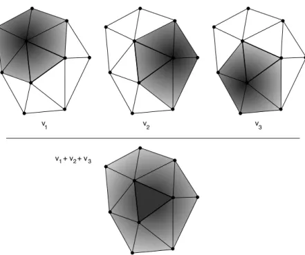
The exitant radiance directions (θ, φ) are parameterized over the hemisphere above each vertex. The surface locations (u, v) are parameterized over the triangle rings cen-tered at each vertex. A triangle ring is the set of triangles which share a vertex. Using triangle rings instead of individual triangles avoids discontinuities at the edges (Chen et al., 2002), but requires that each triangle be represented by three surface maps (one per vertex k). A diagram is shown in Figure 2.5.

The rendering algorithm, which is executed on graphics hardware, evaluates the following function:

Lk(u, v, θ, φ) = rank X

r=1 3

X

k=1

β(u, v, k)g_kr(u, v)hr_k(θ, φ)

(37)

v + v + v ₁ ₂ ₃ v

1 v2 v3

Figure 2.5: The surface functions g(u, v) are parameterized across triangle rings. To get the color for the triangle, each of the three triangle ring functions are weighted byβ(u, v, k) and summed. The weighting function sums to 1.0 everywhere within the triangle. From Chen et al. (Chen et al., 2002).

2.5.2 Visibility and Resampling

The visibility is tested by projecting the triangle mesh using the camera’s position and orientation. Visibility is computed on a per-vertex basis by back-projecting the vertex into the camera. If a point is determined to be visible, the colors are sampled from the input image using bilinear interpolation.

The matrix factorization approach to compression of surface light fields requires that the image data be resampled from the input images to fit into the rows and columns of the data matrices. This resampling occurs in both dimensions; not only are the camera locations at arbitrary locations in the hemisphere, but the projected areas of the triangles vary in each image.

Resampling the images to fill the columns of the data matrix is straightforward. If a triangle ring is determined to be visible, the colors are sampled from the input image using bilinear interpolation.

(38)

Figure 2.6: Resampling of views. Left: The camera positions are projected onto the local basis. Center: Delaunay triangulation of views. Right: Resampling to uniform grid. From Chen et al. (Chen et al., 2002).

the texture maps. Each image represents a point in the hemisphere. The 3D position of the camera is projected onto the vertex basis vectors and normalized. This point is projected down onto the plane and inserted into the Delaunay triangulation. The triangulation is then uniformly resampled at the view map resolution and stored. A diagram is shown in Figure 2.6.

Resampling can cause the amount of data to increase dramatically. In Chapter 3 I discuss methods to avoid this resampling by treating the SLF reconstruction as a scattered data approximation problem.

2.6 Online Methods

Most of the research in image-based modeling has focused onbatch processing systems. These systems process the set of images over multiple passes, and consequently require that the entire set of images be available. For detailed capture of light fields, this requires significant storage (around 106 _{data samples (Hillesland et al., 2003)). In} addition, incorporating additional images into these models requires recomputing the model from the beginning.

(39)

who described a system to interactively capture geometry. The user was incorporated into the processing loop, which enabled them to view the sampling and to steer the solution to eliminate holes in the model.

(40)

CHAPTER 3

Incremental Construction of

Surface Light Fields

The goal of this research is to acquire the appearance of physical objects and render these objects at interactive rates. In contrast to analytical radiance models (Hanrahan and Krueger, 1993; Cook and Torrance, 1982; Oren and Nayar, 1994), the SLF approach has not been widely adopted. I believe that is partially because the capture process is time-consuming and complex.

In this chapter I discuss a system for interactively capturing, constructing, and rendering surface light fields by incrementally building a low rank approximation to the surface light field. Each image is incorporated into the lighting model as it is captured, providing the user with real-time feedback. This feedback enables the user to preview the lighting model and direct the image acquisition towards undersampled areas of the object. We also provide a novel data-driven quality heuristic to aid the user in identifying undersampled regions. Our system reduces the time necessary to capture the images and construct a surface light field from hours to minutes.

3.1 Introduction

(41)

Figure 3.1: A heart figurine, a marble pestle, and a copper pitcher captured and ren-dered with our online system.

These data-acquisition problems can be traced to the lack of feedback during the image capture process, as humans are quite adept at recognizing undersampling errors. An incremental algorithm provides the user with feedback as the lighting model is being constructed, allowing the user to obtain the necessary quality and avoid taking many extra pictures. Examples of several models can be seen in Figure 3.1.

(42)

data-driven quality heuristic to highlight these areas.

We believe this approach has several advantages over other SLF approaches:

• The SLF algorithm we present is fast and incremental. Since each image is pro-cessed as it is captured, the storage overhead is low, and new images can be incorporated at rates of more than one per second.

• The algorithm provides continuous feedback to the user. As a new image is incor-porated into the surface light field, the rendering data structures are immediately updated and displayed, enabling the user to interactively evaluate the light field quality.

• We provide a data-driven quality heuristic to guide sampling. An error metric is interactively computed and displayed to aid in determining which parts of the 4D SLF space are undersampled.

• We provide a structured method for dealing with incomplete data. Due to oc-clusion, many surface patches are only partially visible. Rather than discarding these data, we use the current approximation to fill in these holes.

The core of our approach is the Online SVD (Brand, 2003), a fast memory-efficient algorithm for constructing an incremental low-rank Singular Value Decomposition. The next sections describe the mathematical background of the SVD, then proceed to de-scribe the Online SVD. In Section 3.5, we present details of the implementation, followed by results and conclusions.

3.2 Mathematical Background

Singular Value Decomposition was used by Chen et al. (Chen et al., 2002) to build a compressed representation of the SLF which could be rendered at interactive rates. In this section I describe the mathematical background of the SVD.

3.2.1 Eigenvectors and Eigenvalues

Both the Singular Value Decomposition and Principal Component Analysis are rooted in the concept of eigenvectors and eigenvalues, which are the solutions to the equation

(43)

Figure 3.2: This sequence shows the image acquisition process. The left frame shows an image from the camera. In the middle is the reconstruction before this image is incorporated, with highlights interpolated from nearby views. The right image shows the reconstruction after it is incorporated, with the correct highlights.

where A ∈ _Rn×n_, _x _∈

Rn×1, and λ ∈ R. This equation says that for certain special vectorsx (the eigenvectors), the general transformation matrix A only scales them by a factor (theeigenvalues) and does not rotate them. Every n×n square matrix has n (not necessarily distinct) eigenvectors. They can be found by rearranging the terms of the above equation:

Ax−λx= 0 (A−λI)x= 0

We don’t consider the 0 vector to be an eigenvector, so the above equation is true when

det(A−λI) = 0

This equation is called thecharacteristic polynomial, which is a set ofnlinear equations which can be solved forλto determine the eigenvalues. The eigenvalues are substituted back into the matrix equation to get the eigenvectors. In practice, this is only done for small matrices due to the computational complexity. For larger matrices, an iterative algorithm based on the characteristic polynomial can be used.

3.2.2 Power Iteration Algorithm

(44)

advantage of the property that vectors which are transformed by the matrix A will be scaled in the direction of the largest eigenvector. Initially, the vector is chosen to be some random non-zero vector. This vector is iteratively multiplied by the matrix, which causes it to gradually align with the largest eigenvector. This is repeated until the vector has converged. The eigenvector and eigenvalue are stored, and the eigenvector’s contribution is subtracted from the matrix. The process is then repeated to compute the next largest eigenvector. Here is the pseudocode for determining an eigenvector:

xi = rand(n,1)

xi =xi/kxik

repeat xi−1 =xi

xi =Axi

xi =xi/kxik

until kxi−xi−1k> threshold λi =kxik

To compute the subsequent eigenvalues, the eigenvector is removed from A in a process called Deflation. The outer product of the eigenvector is subtracted from the matrix:

Ai+1 =A−λixixTi

The performance of Power Iteration is highly-dependent on the eigenvalues. The convergence ratio is controlled by the ratio of subsequent eigenvalues λi

λi+1. If this ratio is large, the algorithm will converge rapidly. Thus Power Iteration is usually used only when the first few eigenvalues need to be computed, since these are usually well-separated. Power Iteration was used by Chen et al. (Chen et al., 2002) to determine the eigenvectors of the SLF.

3.2.3 Principal Component Analysis

PCA is a widely used data compression technique in statistics and data modeling (Press et al., 1992). The PCA is computed by determining the eigenvectors and eigenvalues of the covariance matrix. The covariance of two random variables is their tendency to vary together. This is expressed as:

(45)

where E[X] denotes the expected value of X. For sampled data this can be explicitly written out as:

cov(X, Y) =

N X

i=1

(xi−x)(y¯ i−y)¯

N

with ¯x= mean(X) and ¯y= mean(Y). Note that cov(X, X) = var(X), and for inde-pendent variables cov(X, Y) = 0. The covariance matrix is a matrix A with elements Ai,j = cov(i, j). The covariance matrix is square and symmetric. For independent

variables, the covariance matrix will be a diagonal matrix with the variances along the diagonal.

Calculating the covariance matrix from a dataset first requires centering the data by subtracting the mean of each sample vector. Considering the columns of the data matrix A as the sample vectors, we can write the elements of the covariance matrixC as:

cij =

1 N

N X

i=1 aijaji

written in matrix form:

C = 1 NAA

T

Often the scale factor 1/N is distributed throughout the matrix and the covariance matrix is written simply as AAT_.

(46)

0 10 20 30 40 50 60 70 80 0

1 2 3 4 5 6

Term

Eigenvalues of 655x75 data matrix

(47)

3.2.4 Singular Value Decomposition

The Singular Value Decomposition (SVD) is a technique for decomposing a matrix into a set of rotation matrices and a scale matrix. The form is:

A=U SVT

whereA ∈_Rm×n _(with _{m >=}_n),_U _∈

Rm×n,V ∈Rn×n, and S is a diagonal matrix of size _Rn×n. Both U and V are orthogonal.

The SVD is closely related to PCA and to eigenvalue computation. Recall from above the eigenvalue equation:

Ax=λx

In order to compute the eigenvalues, A must be a square matrix. The SVD is less restrictive in that it can be performed on any m×n matrix. The singular values of a matrix A solve the equations

Au =λv and ATv =λu

The vectorsu and v are known as the right- and left-singular vectors respectively. We can show the relation between SVD and eigenvalues through the following equations:

AAT = (U SVT)(U SVT)T =U SVTV SUT =U S2UT

ATA = (U SVT)T(U SVT) =V SUTU SVT =V S2VT

using the fact the U and V are orthogonal so UT ₌ _U−1_{. This shows that} _U _and _V can be calculated as the eigenvectors of AAT and ATA respectively. The square root of the eigenvalues are the singular values along the diagonal of the S matrix.

The advantage of the SVD is that there are a number of algorithms for computing the SVD. One method is to computeV and S by diagonalizing AT_A:

ATA=V S2VT and then to calculate U as:

U =AV S−1

(48)

SVD is a powerful and widely-used compression technique, but it requires that the full set of data be available during processing. Since these data are usually extensively resampled to fit the columns and rows of the data matrices, this can be a significant storage cost. In the next section, we describe an algorithm which can incrementally compute the SVD.

3.3 Online SVD

The Online Singular Value Decomposition (Brand, 2003) is an incremental SVD al-gorithm (Hall et al., 2000; Chandrasekaren et al., 1997) that computes the principal eigenvectors of a matrix without storing the entire matrix in memory. The results are built up from a series of simple operations on the output eigenvectors, which are low-rank approximations to the full matrix. If the low-rank r is much smaller than the size of the matrices, this is a considerable saving, and reduces the computational complexity from quadratic to linear (Brand, 2003).

The Online SVD works as follows (see Figure 3.4). Consider a rank-r SVD

A=U SVT

whereU ∈_Rm×r_, _S _∈

Rr×r, andV ∈Rn×r. Each new column of samples cis projected onto the eigenspace:

j =UTc

The amount that is orthogonal to the eigenspace is given by:

p=c−U j

The norm of this vector, kpk, is a measure of how different the pixels in this new image are from our current approximation. If the pixels are similar (that is, kpk is below a threshold) we can incorporate this new sample by simply rotating the existing eigenspaces.

U0 =U RU V0 =V RV

(49)

!!"!! $ %&'()&*+,

!!"!! - %&'()&*+,

" .

./

.₀ 1

. 2

(50)

the rank to r+ 1 and append the column j to our approximation.

U0 = [U;j]RU V0 =V RV

The rotations are computed by re-diagonalizing the (r+ 1)×(r+ 1) matrix

"

S UT_c

0 kpk

#

→[RU, RV] (3.1)

These rotations can be computed in O(r2). Since only the output matrices U, S, and V are stored, this representation results in significant storage savings.

3.3.1 Error

The batch SVD can iterate over the entire dataset multiple times, while the Online SVD uses only the current approximation and the incoming data vector. Consequently, the Online SVD tends to have more error than a batch SVD for the same rank. Figure 3.5 shows the error as a function of rank. If the rank is too low to approximate the dataset, it will bias the Online SVD by forcing it to select sub-optimal eigenvectors. Brand (Brand, 2003) suggests computing the Online SVD at twice the desired rank and truncating, which allows the eigenvectors more degrees of freedom to fit to the incoming data. This increases the size of the working data structures, but does not affect the size of the rendering data structures.

3.3.2 Missing Values

Acquired radiance data is often incomplete because of occlusion. Many systems are forced to discard surface patches with missing data, or fill in the holes with incorrect values, such as zeros or mean values. A better approach is to estimate the missing data using a process known as imputation. Imputation uses the current Online SVD estimate of the light field to fill in missing values (Brand, 2003). The known samples are projected onto the current eigenspace, and the unknown values are estimated by solving the under-determined system using Linear Least Squares (Golub and Loan, 1996). This fills in the missing values with the nearest plausible values using the Mahalonobis metric (a metric defined in the scaled eigenspace) (Brand, 2003).

(51)

2 4 6 8 10 12 14 16 0

0.2 0.4 0.6 0.8 1 1.2 1.4 1.6 1.8

2x 10

−3

Rank Online SVD

PCA

(52)

example, co could represent the occluded region of a triangle. The current eigenspace

is also partitioned into U+ and Uo. We can set up two linear systems:

U+Sb = c+ UoSb = co

These equations state that a vector b can be projected on the known subspace and the unknown subspace to get the known column vector and the unknown column vector. We can solve these equations using the method of Normal Equations (in (Golub and Loan, 1996) and discussed in Section 4.3.1). The first equation becomes:

b= (SU₊TU+S)−1(SU+Tc+)

This can be simplified using the fact that U is orthogonal:

b = (U+S)−1c+

and substitute UoSk=co

co =UoS(U+S)−1c+

This set of equations yields the full vectorcwhich lies closest to the existing eigenspace in the Least Squares sense (for further details, consult (Brand, 2003)). The inverse is not a true matrix inverse, but is computed using the pseudo-inverse (discussed in Section 4.3.1). Substituting the above equations into Equation 3.1 yields:

"

S UT_c

0 kkk

#

=

"

S S(U+S)−1c+ 0 kc+−UoS(U+S)−1c+)k

#

Figure 3.6 shows the advantage of imputation for surface light fields. In practice, we only impute missing values when at least half of the surface patch is visible in an image. In addition, we can only impute values after 8-10 initial images have been processed, which allows the system to establish a reasonable approximation. A different approach to handle missing data is discussed in Chapter 4.

3.4 Data-Driven Quality Heuristic

(53)

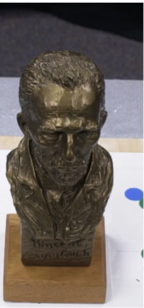
Figure 3.6: Left: The bust dataset with areas of missing data highlighted in red. Right: Imputation of the missing data fills in the areas with plausible values.

information, we developed a data-driven quality heuristic that uses the information obtained from the estimate to indicate whether more data are needed. This is displayed as the user views the model, and provides additional statistics about the reconstruction quality.

One possible way to do this is to assume a fixed BRDF and measure the error be-tween this and the collected samples. This is the approach taken by Lensch (Lensch et al., 2003), who used an uncertainty minimization technique to guide image acqui-sition. We wanted to avoid this fixed BRDF assumption in order to capture a wide variety of reflectance properties.

There are two statistics that we want to provide feedback about: the variation over the surface, and the variation over the viewing direction. To this end, we developed a per-triangle scalar quality heuristic that is computed as the combination of two quality functions:

ψ(s, t, θ, φ) =

q

ψp(s, t)2+ψh(θ, φ)2

The surface quality function ψp measures the quality of the surface approximation

(54)

Figure 3.7: The data-driven quality heuristic ψ(s, t, θ, φ) displayed on the star model. Left: The heuristic is dark in areas where images have already been captured, indicating that the area has been well-sampled. Right: In areas where more data is needed, the heuristic is bright to draw attention to the area.

the new image differs from our approximation. As the SVD refines, the projection error decreases. This scalar quantity is smoothed using an exponential fall-off filter.

The hemisphere quality function ψh is a measure of the sampling density of the

hemisphere. The value is computed by using the areas of the triangles in the Delaunay triangulation of the hemisphere. As more images are captured, the areas of the triangles decrease. The Delaunay triangulation, which is used for interpolation, is described in more detail in Section 4.2.1.

The quality heuristic ψ(s, t, θ, φ) is displayed as a scalar value at each triangle. We display this value in red in our system, since it is easily visible from a distance. An example in shown in Figure 3.7. As the user moves the tracked camera around the object, the object rotates on the screen and the brightness of the heuristic changes. As images are captured in a region, the heuristic darkens and the user moves to a different area. As the light field is being acquired, the user can either view the light field, the heuristic, or a split-screen view of both. In practice, we typically view the camera output and tracking information on one screen and switch between the heuristic and the light field on the other.

3.5 Implementation

(55)

Figure 3.8: A side-by-side comparison of the Buddha model constructed with the OpenLF system (left) and our incremental approach (right). There are some slight differences noticeable in the chest area.

from the physical world and a compressed representation is generated such that it can be rendered at interactive rates on graphics hardware.

The Online SVD enables us to incrementally construct a low-rank approximation to a dataset. In this section we describe how to incorporate this tool into a SLF system. I will first give an overview of the entire SLF capture process, then describe some of the particular components of our system.

3.5.1 The Surface Light Field Construction Process

(56)

structures are updated. The result can then be viewed on the screen, usually after only about 1 second. In addition, the user can view the data-driven quality heuristic as a scalar value for each surface patch, which provides additional statistics about the reconstruction quality.

This section discusses the entire SLF construction process, including the physical setup of the capture environment as well as the software tools that we used to build the systems. Many of the design choices were made for performance reasons to enable the user to view the result of each image acquisition as quickly as possible.

The capture process consists of

1. acquiring the geometry of the object,

2. acquiring a set of images of the object,

3. determining the 3D position and orientation of the camera with respect to the model,

4. determining the visibility of the surface patches,

5. sampling the values from the image,

6. incorporating the values into the representation, and

7. rendering novel images from this representation.

Steps 6 and 7 have been discussed previously in Sections 3.3 and 2.5. The other steps in this process are less complicated, and are described in this section. Since these steps are fairly well-understood in the computer vision community, we used several off-the-shelf components.

The geometry of the object is captured as a preprocess using a FaroTM_digitizing arm. The 3D point samples (usually around 1000-3000 samples) are triangulated using the constrained 3D Delaunay mesh generator Triangle (Shewchuk, 1996). This trian-gulation is then loaded into Blender (Blender, ) or MeshLab (MeshLab, ) for cleanup and refinement. In addition to the 3D model points, the 3D locations of the fiducial markers are also acquired. This enables the model to be registered with the tracking system. An image of the scanning process along with the resulting mesh is shown in Figure 3.9.

(57)

Figure 3.9: Acquiring the geometry of a marble pestle. Left: The object is scanned using a contact scanner. Right: The resulting mesh after triangulation and editing.

a video camera over a digital still camera is the higher speed of data transfer. The camera was calibrated with Bouguet’s Camera Calibration Toolbox (Bouguet, ), and images are rectified using Intel‘s Open Source Computer Vision Library (OpenCV, ).

3.5.2 Pose Estimation

In order to project the image samples onto the geometry, the camera’s position and orientation must be known. The 3D position and orientation of the camera is known as the pose of the camera, and the process of computing it from acquired images is known as pose estimation. To determine the pose of the camera with respect to the object, a stage was created with fiducials along the border. The 3D positions of the fiducials are located in the camera’s coordinate system in real-time using the ARToolkit Library (Kato and Billinghurst, 1999). This library uses image segmentation, corner extraction, and matching techniques for tracking the fiducials. Knowing the 3D position of an imaged fiducial allows the pose of the camera to be computed. When multiple fiducials are present in an image, the camera pose can be refined by minimizing the differences between the pose estimates for each fiducial. A picture of our system showing the fiducials is in Figure 3.11.

(58)

Capture PC Render PC

Pose

Estimation Visibility Resampling PCA Rendering

Real-Time Pose Estimation

Visibility Resampling Online SVD Rendering

Quality Heuristic

Figure 3.10: Top: The OpenLF system. Bottom: Our online system. The two sys-tems share several components, including the visibility, resampling, and rendering. We introduce several new components to convert light field construction into an online process.

Practical surface light fields

ABSTRACT

ACKNOWLEDGMENTS

TABLE OF CONTENTS

LIST OF TABLES

LIST OF FIGURES

LIST OF ABBREVIATIONS

Introduction

1.1

Surface Light Field Capture Difficulties

1.2

Thesis

1.3

Contributions

1.3.1

Incremental Construction

1.3.2

Scattered Data Approximation

1.3.3

Matching Desired Lighting

1.4

Thesis Organization

Background

2.1

Introduction

2.2

Image-Based Modeling and Rendering

2.2.1

Non-Parametric Models

6D

4D

3D

2D

8D

2.3

Surface Reflectance Fields

2.4

Surface Light Fields

2.5

OpenLF

2.5.1

Rendering

(

!

,

"

)

(u,v)

g(u,v)

L(u,v,

!

,

"

)

h(

!

,

"

)

2.5.2

Visibility and Resampling

2.6

Online Methods

Incremental Construction of

Surface Light Fields

3.1

Introduction

3.2

Mathematical Background

3.2.1

Eigenvectors and Eigenvalues

3.2.2

Power Iteration Algorithm

3.2.3

Principal Component Analysis

3.2.4

Singular Value Decomposition

3.3

Online SVD

3.3.1