Remote Sensing of Suspended Sediment Concentration and Hydrologic Connectivity in a Complex Wetland Environment
Colleen McCormick Long
A thesis submitted to the faculty of the University of North Carolina at Chapel Hill in partial fulfillment of the requirements for the degree of Master of Science in the Department of
Geological Sciences.
Chapel Hill 2012
Approved by:
Dr. Tamlin Pavelsky
Dr. Jason Barnes
© 2012
Abstract
Colleen McCormick Long: Remote Sensing of Suspended Sediment Concentration and Hydrologic Connectivity in a Complex Wetland Environment
(Under the direction of Dr. Tamlin Pavelsky)
We use daily MODIS imagery in bands 1 and 2 to monitor suspended sediment and,
by proxy, hydrologic recharge in the Peace-Athabasca Delta, Canada from 2000 to present.
To identify an appropriate suspended sediment concentration (SSC)-reflectance model, we
compare 31 published equations using field observations of spectral reflectance and SSC.
Results suggest potential for spatial transferability of such models if they 1) use of a near
infrared band in combination with at least one visible band, 2) were developed based on
SSCs similar to those in the new site, and 3) are nonlinear. We develop a twelve-year time
series of SSC in Lake Athabasca and observe timing and sources of major sediment fluxes.
We also track the influx of Athabasca River water to floodplain lakes. In three lakes we
identify discharge thresholds required for hydrologic recharge, and we find a significant
Acknowledgements
I am very grateful for the guidance of Dr. Tamlin Pavelsky, whose willingness to
share ideas, knowledge, and time made the completion of this thesis possible. Additional
reviews from Dr. Jason Barnes and Dr. Larry Benninger further improved the final version of
this paper. I also thank Zach Miller, Dr. Larry Benninger, Robert Grandjambe, and the staff
of Wood Buffalo National Park for assistance in the field. Funding for this work came from
the UNC Department of Geological Sciences Martin Fund and the Geological Society of
Table of Contents
List of Tables………...vii
List of Figures…………..……….…………..viii
Chapter 1. Remote Sensing of Suspended Sediment Concentration and Hydrologic Connectivity in a Complex Wetland Environment…………..….1
Abstract………1
Introduction………..2
Study Area: The Peace-Athabasca Delta……….5
Methods………....8
Collection of Field Data………...………..8
Collection and Processing of Satellite Imagery……….9
Evaluation of SSC-Reflectance Models………...11
Analysis of SSC in Lake Athabasca………12
Analysis of Floodplain Lake Recharge………13
Results Spatial Transferability of SSC-Reflectance Models………..…..14
Sediment Dynamics in the Western End of Lake Athabasca……….….16
Tracking Recharge of Small Floodplain Lakes…………...………18
References………..61
Appendix 1: Water quality data and surface velocities………...…………...38
Appendix 2: In situ reflectance measurements………...45
Appendix 3: Sediment Area Index time series for floodplain lakes..……….52
List of Tables
Table
1. Compilation of 31 published SSC-reflectance models
List of Figures
Figure
1. The Peace-Athabasca Delta
2. Athabasca River Discharge, 1970-2011
3. Field data collection sites and study areas
4. Comparison of measured and predicted SSCs for a transect in Lake Athabasca
5. MODIS Reflectance vs. In situ reflectance
6. Analysis time periods and selection method
7. Subset of the 31 tested SSC-reflectance models
8. MODIS-derived sediment maps for the western end of Lake Athabasca
9. Time series of SSC in Lake Athabasca and discharge on the Peace and Athabasca
Rivers
10. Athabasca River discharge vs. SSC in Lake Athabasca and in the Athabasca River
11. Athabasca River discharge vs. Sediment Area Index
Chapter 1:
Remote Sensing of Suspended Sediment Concentration and Hydrologic Connectivity in a
Complex Wetland Environment
Abstract
Maintaining the ecological diversity and hydrologic connectivity of freshwater delta
systems depends on regular recharge of floodplains with river water, which can be difficult to
observe on the ground. Rivers that form deltas often carry large amounts of suspended
sediment, but floodplain lakes and wetlands usually have little sediment in suspension.
Remote observation of high sediment water in lakes and wetlands therefore often indicates
connectivity with the river network. In this study, we use daily 250-m MODIS imagery in
band 1 (620-670 nm) and band 2 (841-876 nm) to monitor suspended sediment transport and,
by proxy, hydrologic recharge in the Peace-Athabasca Delta, Canada. To identify an
appropriate suspended sediment concentration (SSC)-reflectance model, we compare 31
published empirical equations using a field dataset containing 147 observations of SSC and
in situ spectral reflectance. Results suggest potential for spatial transferability of such
models, but success is contingent on the equation meeting certain criteria: 1) use of a near
infrared band in combination with at least one visible band, 2) development based on SSCs
SSC-reflectance model (Spearman’s ρ=0.95), we develop a twelve-year time series of SSC in
the westernmost end of Lake Athabasca, observe the timing and sources of major sediment
flux events, and identify a threshold river discharge of ~1700 m3/s above which SSC in Lake
Athabasca is clearly associated with flow in the Athabasca River. We also track the influx of
Athabasca River water to floodplain lakes, and in three of the lakes identify distinct
discharge thresholds (1040 m3/s, 1150 m3/s, and 1850 m3/s) which result in lake recharge.
For each of these lakes, we find a statistically significant decline in the threshold exceedence
frequency since 1970, suggesting less frequent recharge during the summer.
Introduction
Freshwater deltas are among the most biologically productive and ecologically
diverse terrestrial ecosystems. To sustain their characteristic complexity, these environments
depend on regular recharge with sediment-laden river water, generally through overbank
flooding and flow through distributary channel networks (Lesack et al., 1998). Transport and
deposition of sediment in deltas shapes the landscape through construction of natural levees,
aggradation of wetland areas, and progradation of the delta margin (Syvitski et al., 2009).
Moreover, the movement of water and sediment through delta ecosystems is a key
mechanism for cycling of nutrients and contaminants (Bloesch, 1995; Hernández-Ayón et al.,
1993; Pereira et al., 1996; Owens et al., 2005). Delivery of sediment to deltas worldwide has
declined in the last century due to trapping in upstream reservoirs, artificial construction of
levees, and impacts of climate change (Kummu & Varis, 2007; Syvitski, 2008; Syvitski et
al., 2005; Vörösmarty et al., 2003). These decreases in the amount and frequency of
substantially impact geomorphic and biogeochemical processes in deltas (Meade, 1996;
Yang et al., 2003).
The supply of river water to delta floodplains is largely controlled by hydrologic
connectivity, and an understanding of connectivity is therefore critical to assessing a delta’s
ecological health (Pringle, 2003; Bracken & Croke, 2007). Defining and quantifying
connectivity, however, remain intractable problems in many systems. Metrics used to assess
hydrologic connectivity must often be uniquely chosen based on the catchment under
investigation (Ali & Roy, 2010), and many techniques require extensive fieldwork (e.g.
Fennessy et al., 2004; Jencso et al., 2009; Wolfe et al., 2007). The information these
methods provide can be limited in complex freshwater deltas where small changes in water
level are highly consequential, low slopes lead to frequent reversals in flow direction, and
connections form through small channels or diffuse transport processes. Some previous
studies have used remote sensing to monitor connectivity and effectively bypass the
problems associated with in situ assessments, but most results show general spatiotemporal
variations in the degree of connectivity without fully constraining timing and magnitude of
specific recharge events (e.g. Mouchot et al., 1991; Pavelsky & Smith, 2008; Smith &
Alsdorf, 1998).
Using remote sensing to monitor the presence of high-sediment river water in
floodplain lakes compliments other methods of assessing connectivity by tracking specific
recharge events, even in complex delta systems (Pavelsky & Smith, 2009). Because the
suspended sediment concentrations (SSCs) in delta-forming rivers generally exceed those in
floodplain lakes and wetlands, high-sediment water observed outside of the river often
recharge in freshwater deltas. Because deltas often have highly variable flow conditions and
many lakes and wetlands, frequent and long-term in situ measurements of SSC can be
prohibitively difficult to obtain. Remote sensing is not subject to the challenges of in situ
data collection, and since the 1970s has been used to quantify SSCs in surface waters
(Ritchie et al., 1976).
The amount of sediment in water directly affects the reflectance of solar radiation in
the visible and near-infrared portions of the spectrum; in general, the more sediment in
suspension, the higher the reflectance (Curran & Novo, 1988; Ritchie, 2003). However, the
exact form of the relationship between SSC and reflectance also depends on the mineralogy,
color, and size of the sediments (Novo et al., 1989). These factors can be highly variable in
natural environments, and therefore the applicability of an SSC-reflectance relationship is
generally assumed to be limited to the setting in which the data were collected. Most studies
develop unique relationships by relating field measurements of SSC to reflectance data from
satellite imagery (for examples, Table 1). This purely empirical approach restricts
development of SSC maps from satellite imagery on regional and global scales. A limited
number of previous studies have explored whether models developed in one location are
spatially transferable to another (Holyer, 1978; Ritchie & Cooper, 1991; Topliss et al., 1990)
and suggest that transferability may be possible. However, these studies have focused on low
SSCs (Holyer, 1978) and a limited range of wavelengths (Ritchie & Cooper, 1991; Topliss
et al., 1990), and they do not incorporate work from the past two decades. Development of
one or more spatially transferable models would be of great scientific and practical interest,
but no recent work has compared the applicability of existing models in a common natural
The Peace-Athabasca Delta (PAD) (Figure 1), located in northeastern Alberta,
Canada, is an ideal setting for studying the transferability of SSC-reflectance models. It
exhibits a wide range of SSCs, receives sediment from more than one source, and is often
cloud-free during the summer. Previous work has demonstrated that robust statistical
relationships between SSC and remotely sensed reflectance can be constructed in the PAD
(Pavelsky & Smith, 2009). Furthermore, recent alterations to flow on the Peace and
Athabasca Rivers associated with changing climate and human impacts have raised questions
about how hydrologic recharge in the PAD may be changing. Remote sensing of spatial and
temporal variations in SSC can help address these questions.
This study is comprised of three major components. We first explore the applicability
of published, site-specific SSC-reflectance models to the PAD in order to understand the
extent to which these relationships are spatially transferable. We then use a highly predictive
model to distinguish the source and timing of major sediment flux events in the western end
of Lake Athabasca, which forms the eastern boundary of the PAD. Finally, we use remote
sensing of SSC to determine discharge thresholds above which river water recharges small
floodplain lakes in the PAD and examine changes in the exceedence frequency of these
thresholds.
Study Area: The Peace-Athabasca Delta
The Peace-Athabasca Delta is a hydrologically complex and ecologically diverse
freshwater delta formed by the confluence of the Peace, Athabasca, and Birch Rivers near the
western end of Lake Athabasca (Figure 1). The three intersecting river deltas cover ~5,200
United Nations Educational, Scientific, and Cultural Organization (UNESCO) World
Heritage site and a Ramsar Convention Wetland of International Importance because of its
biological significance and role as the largest alluvial-wetland habitat in the region. The
delta provides a habitat for migratory birds and land mammals including moose, black bear,
and wood buffalo (Prowse & Conly, 2002). The wildlife and vegetation in the PAD also
have cultural and historical importance to indigenous residents in the region, including the
Athabascan Chipewyan and Mikisew Cree First Nations. A large portion of the delta (~80%)
is protected within Canada’s Wood Buffalo National Park. However, the PAD depends on
the rivers that flow into it to support its aquatic and terrestrial habitats, and natural or
anthropogenic changes in river flow far upstream can have significant effects on the delta.
During normal flow conditions, the main source of recharge to the delta is the
north-flowing Athabasca River, and drainage is northward through several distributaries to the
Peace River and, ultimately, the Slave River. However, if the water level on the Peace River
is higher than that of Lake Athabasca, flow reverses along the distributary channels that
connect the Peace River to the lake. The relationship between flow on the Peace River and
the hydrology and ecology in the Peace sector of the delta have been addressed by several
studies since the 1970s in response to the completion of the W.A.C. Bennett dam, which
regulates flow from the headwaters of the Peace River (Farley & Cheng, 1986; Leconte et al.,
2001; Peters & Prowse, 2001; Prowse & Demuth, 1996). There is some evidence that flow
regulation has decreased the frequency of ice jam flooding on the Peace River, which is the
primary mechanism of very large-scale flooding in the PAD (Beltaos et al., 2006a; Beltaos et
al., 2006b). Between 1959 and 1976, major ice-jam flooding occurred four times in
in 1996 and 1997 (Beltaos et al., 2006a). As a result, the dominant sources of recharge in
recent decades have been springtime ice jam floods and summertime high water events on
the Athabasca River (Pavelsky & Smith, 2008; Peters et al., 2006; Töyrä & Pietroniro, 2005).
Since the 1970s, summer discharge on the Athabasca River has declined (Figure 2)
due to both natural and anthropogenic forces. Increased evapotranspiration and diminished
contributions from snowpack and glaciers in the Canadian Rockies, likely related to
anthropogenic climate change, are responsible for much of this decline (Schindler, 2001;
Schindler & Donahue, 2006). Increasing water withdrawals for industrial operations in the
Alberta Oil Sands (located on the Athabasca River about 250 km upstream from the PAD)
could add to future discharge declines (Schindler & Smol, 2006), though winter, not summer,
is the key time of year for assessing the ecological impacts from oil sands withdrawals
(Andrishak & Hicks, 2011). The effects of this decline on hydrologic recharge in the PAD
are largely unknown. In particular, the thresholds of discharge required to deliver river water
to ecologically important floodplain lakes remain unquantified.
Recharge of floodplain lakes in the Athabasca sector of the PAD occurs when flow on
the Athabasca River rises sufficiently to either overtop its levees or reverse flow on the small
channels that ordinary are directed into the river from floodplain lakes. Except during
recharge events, SSCs are higher in the Athabasca River than in floodplain lakes. As a
result, the presence of high sediment water in a floodplain lake represents, under most
circumstances, an input of river water. A detailed time series of SSCs in these lakes would
provide information about how hydrologic recharge in the PAD is responding to the
decreases in discharge on the Athabasca River. Pavelsky and Smith (2009) used satellite
and related timing of recharge to discharge on the Athabasca River. We expand on this work
by examining SSC in Lake Athabasca and determining the threshold discharge values
required for hydrologic recharge of floodplain lakes.
Methods
Collection of Field Data
During a field season from June 20th to July 7th, 2011, we measured spectral
reflectance and water quality in lakes, rivers, and distributary channels in the PAD. In-situ
measurements of temperature (°C), color dissolved organic matter concentration (µg/L),
turbidity (NTU), chlorophyll content (µg/L), and specific conductivity (µS/cm) were
collected using a Eureka Manta Multiprobe a total of 147 times at 71 unique locations
(Figure 3). Multiprobe measurements were collected at two-second intervals for at least
three minutes and averaged to obtain one value for each variable per site. Surface flow
velocity was measured at most river locations (67 total measurements) using a stopwatch, a
handheld GPS, and a small drogue (following Pavelsky and Smith, 2009). These datasets
augment water quality data collection in the PAD beginning in 2006 and continuing in 2007,
2010, and now 2011. The 2006-2007 data is archived at the Oak Ridge National Laboratory
Distributed Active Archive Center for Biogeochemical Dynamics and is available at
http://daac.ornl.gov//HYDROCLIMATOLOGY/guides/PAD.html.
Spectral reflectance from the water surface was measured at 1 nm intervals between
350 and1025 nm at each of the 147 field sites using an ASD FieldSpec® 3 Portable
Spectrometer with an attached OL 731 Smart Detector for solar irradiance measurements. A
location prior to collection of reflectance spectra to account for changes in lighting
conditions between sites. Three reflectance measurements were collected at each location
and then averaged to obtain one reflectance value per wavelength per site.
Suspended sediment concentrations were also measured at each site. We collected
275 mL water samples from the top ~15 cm of the water column. Water samples were
filtered onto pre-weighed 1.2 µm Millipore cellulose filters using a vacuum filtration system.
After filtration, the filters were dried in an oven at 100° C for 30 minutes and then reweighed
on a high precision balance to determine the weight of total suspended matter. This weight
divided by the sample volume yielded the suspended sediment concentration (mg/L).
Collection and Processing of Satellite Imagery
Previous studies have used high resolution satellite imagery to track variations in SSC
in wetland environments (e.g. Doxaran et al., 2002; Mertes et al., 1993; Ritchie & Cooper,
1991). Because of infrequent temporal sampling, however, such imagery is unsuitable for
tracking SSC in the PAD on daily to weekly timescales. We therefore use imagery from
NASA’s two Moderate-resolution Imaging Spectroradiometer (MODIS) sensors, which each
provide daily observations. Many previous studies have found that a combination of red and
near-infrared bands, such as MODIS band 1 (red; 620-670 nm) and band 2 (near-infrared;
841-876 nm), results in robust quantification of SSC (e.g. Doxaran et al., 2009; Holyer, 1978;
Novo et al., 1989). Additionally, MODIS bands 1 and 2 have sufficiently high spatial
resolution (250 m) in the red and near-infrared bands to detect moderate-sized floodplain
Daily MODIS Level 2G Aqua and Terra scenes (MOD09GQ) collected over the PAD
were downloaded using NASA’s Warehouse Inventory Search Tool
(http://wist.echo.nasa.gov) for every summer (May-September) from 2000 through 2011. A
total of 3,672 images were obtained. The Aqua satellite was not launched until 2002, and
therefore for 2000-2002 only one MODIS-Terra image per day is available. All MODIS
Level 2G scenes are radiometrically and geometrically corrected for variations in sun and
sensor angle and atmospheric conditions. Scenes were projected into UTM Zone 12N/WGS
84, and the dataset was automatically filtered to remove scenes where the PAD is more than
30% cloud covered based on a band 1 reflectance threshold of 0.15 (following Chen et al.,
2009). Elimination of cloudy images yielded 1,620 total images suitable for analysis.
Most data collection points in PAD rivers are not visible in MODIS imagery because
the spatial resolution is too coarse. Among the 147 field data collection points, though, is a
twenty-three point transect in the western end of Lake Athabasca, and MODIS pixels
corresponding to these points are free of land contamination (Figure 4a). We use data from
these points to directly validate MODIS-derived reflectance and SSC against field
observations. Reflectance data was extracted from MODIS bands 1 and 2 for the 23 transect
points, and comparison of the Band 2/Band 1 ratio with same-day in situ reflectance at the
same wavelengths shows a high correlation (r=0.91) and little bias (p=0.08 using a paired
Student’s t test) (Figure 5). A ratio is used for this comparison to account for atmospheric
variations over short spatial scales that are not addressed by the large-scale corrections
applied to the MODIS images. The high correlation suggests that in situ reflectance can be
used to test the applicability of empirical SSC-reflectance models to the PAD, and models
Evaluation of SSC-reflectance models
In order to determine if an existing SSC-reflectance model can be applied in the PAD,
we evaluate the spatial transferability of 31 published SSC-reflectance empirical
relationships representing a range of hydrologic environments including rivers, inland lakes,
estuaries, deltas, and bays. Some models predict turbidity instead of SSC, but as in many
discussions of remote sensing of SSC (e.g. Duane Nellis et al., 1998; Wass et al., 1997) we
treat both metrics interchangeably. We use 147 in situ spectral observations from the PAD to
estimate SSC using each model and compare the results against in situ SSC measurements.
Because the relationships often contain outliers and are sometimes non-linear in form,
Spearman’s ρ (Spearman, 1904), a nonparametric test of correlation, is a more appropriate
measure of covariance in this case than is Pearson’s r. Collectively, the models in Table 1
were developed using SSCs from <10 to 2250 mg/L, but most individual studies are limited
to a narrow range of concentrations. The 147 field measurements of SSC in the PAD range
from 3.9 to 3602 mg/L, and no previous work has tested the applicability of SSC-reflectance
models across such a wide range of concentrations.
Some models predict SSCs that are highly linearly correlated with measured values
but are numerically dissimilar. In order to improve these models’ predictive capacity, we
perform linear regressions between measured and modeled values and divide the modeled
values by the slope of the regression line. These scaling factors may be required in part
because of physical differences in the sediment color and grain size among different
locations. It is also possible that in some studies reflectance is scaled differently (e.g. as a
Analysis of SSC in Lake Athabasca
Among the most highly predictive models is one developed by Doxaran et al., (2009)
specifically for MODIS data (see section 4.1). We use this model to analyze sediment
dynamics in the western end of Lake Athabasca using MODIS imagery from summers
2000-2011. To monitor time series of sediment input to Lake Athabasca from the Peace and
Athabasca Rivers, we establish two virtual sediment gauges in the western end of Lake
Athabasca: one at the terminus of the Athabasca Delta, and a second on the north shore of
Lake Athabasca in an area that generally receives high sediment water only from the Peace
River (Figure 3). To create these virtual gauges, we quantify SSC for three horizontally
adjacent pixels at each location and then use the median value to represent the SSC. We
remove images where any of the six gauge pixels are cloud covered (Band 1 > 0.15).
Previous work suggests that SSC-reflectance models are time invariant in a localized
environment so long as the source of sediment remains the same (Dekker et al., 2001;
Ritchie, 2003), and we use the scaled Doxaran et al., 2009 equation to develop time series of
SSC at both virtual gauges for each summer from 2000-2011 with daily to weekly temporal
resolution (on average, ~40% of days per summer were suitable for inclusion).
We compare the SSC time series from the two virtual gauges to daily river discharge
measurements on the Peace and Athabasca Rivers. River discharge data was obtained from
Environment Canada for the gauge stations Athabasca below McMurray (Station ID:
07DA001) and Peace at Peace Point (Station ID: 07KC001). We apply a three-day lag to the
Athabasca River discharge data to account for the ~250 km distance between the gauge and
the PAD. The optimal lag of three days is based on 1) calculations with surface flow velocity
between 84 SSC measurements in the Athabasca River and river discharge with 0, 1, 2, 3,
and 4 day lags. The three-day lag gives the highest R2 value (0.88) in the regressions. The
gauge for the Peace River is about 155 km away from Lake Athabasca, but because flow
dynamics are complicated and often reverse in this reach of the river, we were unable to
determine a consistent lag. Instead, we use same-day discharge for the Peace River.
Analysis of Floodplain Lake Recharge
We manually select six floodplain lakes that are consistently visible in MODIS
images (Figure 3) to determine Athabasca River discharge thresholds above which river
water is consistently delivered to floodplain lakes in the Athabasca sector of the PAD. We
are unable to quantify SSCs in these lakes with the model used in Lake Athabasca because
the spatial resolution of MODIS results in mixed pixels contaminated by vegetation or bare
soil in most of the small floodplain lakes. Instead, for each clear-sky MODIS image we use a
binary metric to monitor Sediment Area Index (SAI), the proportion of lake area containing
high sediment water (following Pavelsky and Smith 2009). To calculate SAI, we create
individual masks of each lake, and remove images in which any masked pixel is
contaminated by cloud. For each lake in each remaining image, we count the number of
water pixels (defined as MODIS Band 2 < 0.05) and the number of high sediment water
pixels (defined as MODIS Band 1 – Band 2 > 0.01). The sizes of the lakes vary temporally,
and analyses for each lake are limited to days when lake area exceeds 0.25 km2 (4 inundated
pixels). The number of high-sediment water pixels divided by the total number of water
We compare the SAI time series for each lake to discharge on the Athabasca River on
days during the rising limb of the first major summertime hydrograph peak. These events
(one per year) are found by identifying all points of inflection on the hydrograph and then
selecting the first event after June 1st when discharge increases by at least 60% between two
inflection points (for example, Figure 6). As water rises in the Athabasca River, it recharges
the floodplain lakes at specific stage thresholds, but once recharge has begun the sediment
and water dynamics become much more complex. As such, it is during this first summertime
high water event that we are most likely to cleanly identify a recharge threshold. After
discharge reaches a maximum, the decline in river discharge and the decline in SSC in the
lake do not happen at the same rate, so only the rising limb of the peak is used here. We do
not consider peaks before June 1st to avoid the effect of early spring floods related to ice
jams, in which water levels, sediment concentrations, and river discharge are often
decoupled. The timing and duration of each event are shown in Figure 6. In 2001, we
manually extend the analysis period by 4 days because of a one-day 9% decline during the
rising limb of the hydrograph.
Results
Spatial Transferability of SSC-Reflectance Models
Our results confirm that it is possible to predict SSCs in the PAD using models
developed elsewhere; several models produce estimates of SSC that are highly correlated
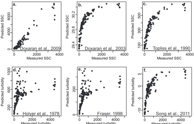
with our validation dataset (Table 1). Among the highly predictive models, the form of the
best-fit relationship between observed and predicted SSCs varies, and it often has a power
only one to produce values that are linearly correlated with the validation dataset across the
entire range of SSCs observed in the PAD (Figure 7a). This equation, with a scaling factor
of 2.9 applied, accurately predicts SSCs using both in situ reflectance measurements and
satellite-based reflectance from MODIS Terra and Aqua (Figure 4b). Comparing measured
SSCs to those predicted with this model results in a better R-squared value for the PAD
(0.94) than for the Gironde Estuary (0.89), where the model was developed. Some other
models produce values that are linearly correlated with the validation dataset at low
concentrations (i.e. <~200 mg/L), but become nonpredictive at higher concentrations (Figure
7 d,e). For all cases in which the best-fit relationship is linear, application of a correction
factor based on the slope of the linear regression between the observed and modeled data is
necessary to reproduce observed SSC values.
Although some models do accurately predict SSCs in the PAD, values from the
majority of the models do not closely match the validation dataset. Some produce negative
values for SSC or turbidity (e.g. Fraser, 1998; Song et al., 2011; Islam et al., 2001; Hellweger
et al., 2006) (Figure 7f), others give values orders of magnitude different from our
measurements (e.g. Aranuvachapun & Walling, 1988; Dekker et al., 2001; Keiner & Yan,
1998; Lathrop et al., 1991; Hellweger et al., 2006), and many are poorly correlated with field
measurements. Differences in mineralogy, sediment color, and sediment size can likely
explain some of the limited predictive power of these models in the PAD, but it is surprising
that many models offer no predictive capacity given the positive relationship between SSCs
and spectral reflectance that forms the basis for all of the models.
Comparing the successful models to those that are ineffective suggests three main
for spatial transferability: 1) the use of a combination of a near infrared band with one or
more visible bands, 2) development based on SSCs with a maximum similar to the maximum
SSC observed in the PAD, and 3) a nonlinear equation form. The six best models (all with
ρ≥0.95) were developed using maximum SSCs of at least 1000 mg/L and a combination of
reflectance in a near infrared and a visible band. The seventh best, though calibrated for less
turbid waters, also uses a near infrared band along with visible bands. Of the remaining 24
models, 16 use only a single band, 7 use a combination of bands but do not include a near
infrared band, and 1 uses a combination of bands not including a visible band. Finally, out of
the nine linear equations tested, only one is in the top ten (Fraser 1998), suggesting that
non-linear models are preferable for modeling SSCs in the PAD.
Our results indicate that spatial transferability of a model is most likely to be
successful if the model meets all three proposed criteria. Models that meet only one of these
criteria (e.g. they predict high SSCs using one band alone, or have a nonlinear form but were
developed to model only low SSCs) produce weaker correlations. Strong performance of a
model in predicting SSCs in the PAD does not indicate universal transferability, but the
characteristics of high-performing models identified here can be used to guide model
selection in environments where in situ measurements are unavailable to calibrate
site-specific relationships.
Sediment Dynamics in the western end of Lake Athabasca
To understand the dynamics of water input to Lake Athabasca by the Peace and
Athabasca Rivers, we created daily sediment maps of the westernmost end of the lake
sediment-laden river water input to the lake. We can also distinguish the source of river
water delivered to the lake using virtual sediment gauges near the lake’s two sources of
inflow (i.e. the Peace and Athabasca Rivers) (Figure 4). Comparison of SSC time series
from these two locations (Figure 9) reveals temporally separate peaks in SSC indicating the
source of river water during major flux events. The Athabasca River always flows into Lake
Athabasca, but we also identify two instances, in May 2007 and July 2011, where peaks in
SSC at the northern shore of the lake indicate inflow of Peace River water.
There is an observable relationship between the timing of significant peaks in SSC in
Lake Athabasca and peaks in Athabasca River discharge (Figure 9). Parallels between
fluctuations are difficult to detect for small variations in SSC and at low discharge, but the
largest peaks in discharge do cause peaks in SSC, most notably in 2001, 2007, and 2011. To
better understand the relationship between these two variables, we examine data from the
rising limb of the first summertime hydrograph peak, the same metric used to identify inflow
thresholds for small lakes (Figure 6). As with small lakes, it is during these events that SSC
in Lake Athabasca is most likely to reflect river discharge instead of wind, biological
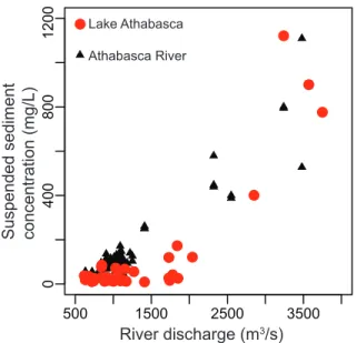
activity, or other confounding variables. Results suggest an Athabasca River discharge
threshold of ~1700 m3/s at which Lake Athabasca SSCs near the Athabasca Delta begin to
increase dramatically from ~200 mg/L to a maximum of 1085 mg/L at an Athabasca River
discharge of ~3200 m3/s (Figure 10). Our compilation of 12 years of near-daily data shows
that at discharges less than ~1700 m3/s, SSCs remain below ~100 mg/L and are uncorrelated
with Athabasca River discharge.
In order to determine the sensitivity of this result to the SSC virtual gauge location,
Delta. The relative values of SSC varied predictably (i.e. higher closer to shore and lower
out in the lake), but at all locations the same discharge threshold of ~1700 m3/s was apparent.
Such a threshold is not observed between SSCs in the Athabasca River and river discharge,
however. In this case, the variables are linearly correlated (r=0.94) even at low discharges
(Figure 10). Finally, we examined the equivalent dataset for the Peace River and find no
correlation between river discharge and SSC at the Peace River virtual gauge. This is likely
because input of Peace River water depends on the relative levels of the river and Lake
Athabasca and not only on river discharge.
Tracking Recharge of Small Floodplain Lakes
Athabasca River water is input to Lake Athabasca under all flow conditions, but
summertime recharge of ecologically important floodplain lakes occurs only when river stage
is sufficiently high. To identify discharge thresholds which consistently initiate recharge in
individual lakes, we compare Athabasca river discharge during the time periods identified in
Figure 6 with the Sediment Area Index of six floodplain lakes consistently visible in MODIS
imagery (Figure 11). Positive relationships between Athabasca River discharge and SAI are
apparent in Lakes 1, 2, and 3. For each of these lakes, there is a distinct discharge threshold
above which there is always high sediment water present and below which there is little to no
high sediment water. We know from field observations that these three lakes are
hydrologically connected to the Athabasca River through small distributary channels which
sometimes, but not always, flow into the lakes. Often, water flows very slowly out of the
lakes and back to the river. The threshold values likely represent the discharges at which
High sediment water was detected in Lake 4 on just two days, neither of which
corresponds to high discharge. This lake is likely disconnected from the river system by
natural levees that are not overtopped even during high flow events. In Lakes 5 and 6, there
is some suggestion of a threshold discharge value above which SAI is always greater than 0,
but the relationships for these lakes are complicated by the presence of many instances of
high SAI and low river discharge. We know from field observations that Lakes 5 and 6, like
Lakes 1, 2, and 3, are hydrologically connected to the Athabasca River through distributary
channels. The apparent discharge thresholds on Lakes 5 and 6 may represent inflow of river
water. In these lakes, however, other factors that are not as influential in Lakes 1, 2, and 3,
such as resuspension of lake-bottom sediments by wind, likely increase SAI without
influence from the river.
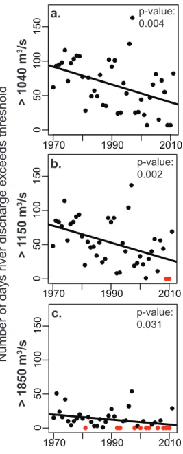
The river discharge thresholds for inflow of water to the three high river-influence
lakes are 1040 m3/s (Lake 1), 1150 m3/s (Lake 2), and 1850 m3/s (Lake 3). Previous studies
have explored hydrologic connectivity in the PAD and have yielded qualitative measures of
floodplain lake connectivity (e.g. Pavelsky & Smith, 2008; Prowse & Demuth, 1996; Wolfe
et al., 2007), but no other study has previously identified discharge thresholds required for
recharge. We use these thresholds to identify the number of days in each year since 1970 on
which Athabasca River discharge is sufficiently high to recharge each lake (Figure 12).
Because lake recharge often depends on relative water surface elevations in the river and
lake, recharge likely did not occur on all days above this threshold, but a higher number of
days above the discharge threshold likely implies greater overall recharge. Since 1970, there
has been a statistically significant (p<0.05) decrease in recharge frequency for each of the
recharged in all years, and Lake 3 was recharged in every year except 1981 (Table 2). In
contrast, during the second half of the study period (1991-2011) discharge on the Athabasca
River failed to reach the threshold required to recharge Lake 2 three times, and the threshold
for Lake 3 was met in just ten of the twenty years.
Discussion and Conclusions
The first principal conclusion of this study is that models for remotely sensing SSC
developed in one location can, in some cases, be transferred to another location. The first
criterion we identify for making such a transfer (i.e., that a near infrared band and a visible
band used in combination are more effective than a single band used alone or another sort of
combination) is supported by previous work also suggesting that multispectral models are
preferable for remotely sensing SSC (e.g. Holyer, 1978; Schiebe et al., 1992; Topliss et al.,
1990). Some previous studies (e.g. Doxaran et al., 2002; Holyer, 1978; Novo et al., 1989)
have more specifically suggested that the best models use a combination of a near infrared
and a red band. In our study, the model that produces the best linear correlation with our
field dataset uses this combination, but five of the top seven models use a near infrared band
paired with a green or blue band. This suggests that bands in the green and blue part of the
spectrum may be just as effective as red bands for remotely sensing SSC as long as they are
paired with a near infrared band.
Our results suggest that models developed using comparatively low SSCs have
limited success predicting the higher SSCs in the PAD, while models based on higher SSCs
are more effective. This finding is corroborated by past studies, which have found that
which work well at low concentrations can saturate at higher concentrations (e.g. Ritchie and
Cooper, 1988; Ritchie et al., 2003; Chu et al., 2009; Topliss et al., 1990; Holyer et al., 1978;
Han and Rundquist, 1994). Some of the models we test are also predictive for low SSCs but
then become saturated at higher concentrations (e.g. Doxaran et al., 2003; Topliss et al.,
1990; Song et al., 2011) (Figure 7 d,e). Holyer et al., (1978) found that saturation occurs
when using reflectance in the red band, but using a near infrared band along with a red band
corrects this problem. In contrast, our analysis shows no discernible pattern in which spectral
bands were used among models that saturate. We suggest instead that the gap between the
maximum SSC from which these models were developed and the much higher SSCs we
observe in the PAD may result in saturation at high SSCs.
Finally, we suggest that nonlinear models may be more successful for predicting
SSCs in a new location than other forms. Past studies suggest that linear relationships are
effective for remotely sensing SSCs less than 50 mg/L, but for values greater than this,
curvilinear relationships are necessary (Ritchie et al., 2003). In the PAD, we found that
exponential relationships worked the best. This is likely because of the large range of SSCs
in the PAD, and for different environments other nonlinear forms may also work well. In
environments where SSCs are relatively low, the form of the relationship may not be as
significant when selecting a model; Ritchie & Zimba, 2006) noted that for SSCs between 0
and 50 mg/L, reflectance from almost any visible or near-infrared wavelength is linearly
related to SSC. Nevertheless, in the PAD, where SSCs range from less than 5 to more than
3000 mg/L, equation form is an important factor influencing success of models in predicting
If the three primary conditions identified here are not met, then application of an
SSC-reflectance relationship beyond its area of development may produce unreliable results.
Even when these requirements are met, it remains necessary to develop a constant correction
coefficient, obtained from a linear regression between observed and modeled SSCs, to
account for location-specific differences in factors like sediment color and grain size. If
limited availability of in situ data prevents development of such a correction, it remains
possible to accurately observe relative differences in SSC. For much of our work focusing
on spatial and temporal patterns of SSC, relative SSC measurements would be fully
adequate.
The scaled equation from Doxaran et al., (2009) which we use to map SSC in Lake
Athabasca is substantially more sophisticated than prior models used in the PAD (Pavelsky
& Smith, 2009), and it fully addresses anomalously high predicted SSCs from that work
associated with biological activity. Our results allow us to distinguish between
sediment-laden river water input from the Peace and Athabasca Rivers for major flux events. Input of
Peace River water to Lake Athabasca is not directly controlled by discharge from the river,
depending instead on the relative water levels of the river and the lake (PAD-PG, 1973). If
the lake level is lower than the river level, the Peace River will flow into the lake regardless
of river discharge. Though it is not possible to predict the input of Peace River water to Lake
Athabasca using river discharge alone, remote monitoring of SSC allows us to track
occurrences of inflow in the absence of in situ monitoring.
In contrast to the Peace River, the Athabasca River always flows into Lake
Athabasca, and we expect to observe a relationship between discharge and input of river
discharge less than ~1700 m3/s and SSC less than ~100 mg/L, which suggests that river
discharge is not the only important control on SSC in Lake Athabasca. Wind almost
certainly also influences SSC at the water surface through resuspension of bottom sediment
and mixing of lake and river water, and at low discharges it may overwhelm the river signal.
It is also possible that when discharge is less than 1700 m3/s, sediment settles out of
suspension within the river itself before reaching the lake. At high discharge values,
however, input of high sediment water appears to overcome these confounding factors and
SSC becomes more strongly related to discharge.
Even at the lowest discharges, Athabasca River water flows into Lake Athabasca, but
this is not always the case in the small floodplain lakes in the PAD. We assess the
connectivity of six of these floodplain lakes to gain a more thorough understanding of
recharge in the delta. Prowse and Demuth (1996) examined hydrologic connectivity in the
PAD and divided the delta into regions of “open,” “restricted,” and “isolated” drainage based
on the work of Jaques, and PAD-PG (1973). Based on these classifications, our high
river-influence and strongly connected lakes (Lakes 1-3) as well as two of our low river-river-influence
lakes (4 and 6) are in “restricted” zones. Lake 5, which we found to be more connected to
the river than Lake 4, is in an “isolated” zone. Wolfe et al. (2007) use the same three
classifications as Prowse and Demuth (1996) and also include a fourth category for very
shallow, rainfall-influenced lakes. They base their classifications on δ18O-derived
evaporation-to-inflow ratios and examine three of our six study lakes: Lakes 2 and 3 are
defined as “open,” and Lake 5 is defined as “restricted.” Our results agree more closely with
the classifications of Wolfe et al. (2007) than with those of Prowse and Demuth (1996).
principal advantage of the method used here is that it allows us to identify specific
occurrences of lake recharge and thus determine discharge thresholds on the Athabasca River
associated with lake recharge.
The three lakes most proximal to Lake Athabasca are the low river influence lakes,
and it is likely that the lake level in Lake Athabasca strongly influences the amount of water
and sediment they receive, especially when lake levels are high (Pavelsky & Smith, 2008;
Peters et al., 2006). The low river influence lakes are also significantly shallower than the
high river influence (Smith & Pavelsky, 2009) and sediment re-suspension due to wind likely
interferes with the river discharge signal. Bottom-reflectance may also impact remote
measurement of SSCs in these shallow lakes. Our results are in accordance with the findings
of Pavelsky and Smith (2009), who found that suspended sediment in Lake 5 did not closely
mirror discharge in the summer months, as well as with Prowse and Demuth (1996), whose
classification shows Lake 5 as an “isolated” basin that is significantly recharged only by
overbank flooding. Pavelsky and Smith (2008) noted that Lake 5 was hydrologically
connected to the river system in 2007; our observation of an apparent threshold is in
accordance with this finding, since in 2007 Athabasca River discharge exceeded the apparent
threshold required to recharge Lake 5.
The identification of threshold discharges required to recharge lakes that are strongly
influenced by the Athabasca River is valuable for understanding the effects on the PAD of
declines in flow on the Athabasca River. In the past four decades, we have observed a
substantial decline in the number of days on which Athabasca River discharge is sufficiently
high to recharge the floodplain lakes studied here. In particular, recharge from the Athabasca
also suggest that if summer discharge on the Athabasca River continues to decline at the
current rate, many small floodplain lakes (e.g. Lakes 1-3 in our analysis) will no longer be
recharged with Athabasca River water except during the spring ice-jam flood period by
approximately the 2040s, and possible as early as the 2020s in the case of Lake 3.
Transformation of the Athabasca portion of the PAD from a frequently to an infrequently
flooded environment has the potential to substantially affect delta ecology and biological
productivity (McGowan et al., 2011; Prowse & Conly, 2002; Wiklund et al., 2011). A
reduction in the frequency of recharge would allow willow (Salix sp.) and shrub communities
to overtake more productive grass- and sedge- dominated environments that currently serve
as habitats for migratory birds (Timoney, 2006; Töyrä & Pietroniro, 2005). Those lakes
identified as highly river-influenced (i.e. Lakes 1, 2, and 3) are likely to face the most
changes in their ecology and productivity, and all of these effects could be amplified by
continued climate change or increased water withdrawals on the Athabasca River for use in
Figures
Figure 1. Landsat image of the Peace-Athabasca Delta. Inset (from Pavelsky and Smith, 2009) shows location of the delta in Canada.
Figure 2. Mean summer (June-July-August) discharge on the Athabasca River below Fort McMurray from 1970-2011. Dashed line shows statistically significant decline in discharge over the time period.
!"#$%
!"#$%&'(")"*+" CANADA
&'()'* +,-(.(/)(
0'1,(
#2($'# #####31(45'
2($' +,-(.(/)(
61(7'#847'561(7'#847'5
+,-(.(/)(# 847'5
+,-(.(/)(# 847'5
&'()'# 847'5
&'()'#
847'5 8474'5'#9'/
8:)-'5/ 8474'5'#9'/
8:)-'5/ 3-';(1#9'/
<=(,5'#>:=5)-'/ 3-';(1#9'/ <=(,5'#>:=5)-'/
!"#$ %&'()*&#+
!""
#"""
#$""
#%""
#&'" #&%" #&&" (""" ("#"
)*+,-.-/*01-2,3+-45678390,-:;
<=6>
Figure 3. Landsat image of the central PAD showing the 71 locations where field data was collected in 2011. Outlined are the six small lakes referenced in Figures 11 and 12. Stars mark the locations of the virtual SSC gauges where the values in Figure 9 were calculated.
!
"
#
$
%
&
!"#$%$&'$( )*+,-
.,$',()*+,-''''''()*)'+,--.+*/,0'1,/0*2
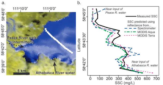
Figure 4. (a) False color MODIS image from the Terra platform obtained on June 27, 2011. Transect of 23 points where field measurements of SSC and reflectance were collected are shown in white. (b) Comparison between measured SSCs and those predicted using same-day reflectance from the spectrometer, MODIS Terra, and MODIS Aqua as inputs to the model from Doxaran et al., (2009) scaled for the PAD.
Figure 5. Comparison between the Band 2/Band 1 reflectance ratio from MODIS imagery and from field spectrometer measurements. Close fit to a 1:1 line verifies transferability of models between reflectance data sets.
0 100 200 300 400 500 600 700
58
o42’0”
58
o45’0”
58
o43’30”
SSC (mg/L)
Near input of Peace R. water
Latitude
Near input of Athabasca R. water
Measured SSC
MODIS Terra MODIS AquaSpectrometer SSC predicted using reflectance from...
! !!
! ! !
! !! ! !
! ! ! !! !
! ! ! !! ! !!
!! !
! ! ! ! !
!! !
! ! ! !!
! ! !
! !! ! ! !
! !! ! !
58
o42’0”
58
o45’0”
58
o48’0
”
58
o39’0”
5 km
Peace River water (intermittent)
Peace River water (intermittent)
Athabasca River waterAthabasca River water
111o10’0” 111o0’0”
a. b.
!"!#$%&'
()( ()* ()+ (), ()- !)(
()(
()*
()+
(),
()-!)(
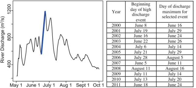
Figure 6. River discharge on the Athabasca River below Ft. McMurray in 2002 as an
example to show metric used for analyses. Bold, highlighted portion indicates the rising limb of the first summertime (after June 1) hydrograph peak (defined as an increase of >60% between inflection points). Table shows timing and duration of all such events for 2000-2011.
!""
#""
$%""
&'()*+,'-./0*1)+23
45-6
708+$ 9:;)+$ 9:<8+$ =:1+$ >)?@+$ A.@+$ +
+
Year
Beginning day of high
discharge event
Day of discharge maximum for selected event
Figure 7. Subset of the 31 SSC-reflectance models used to model SSC data in the PAD. Plots show the relationship between measured values for SSC (mg/L) (a-c) or turbidity (NTU) (d-f) on the x-axis and predicted values on the y-axis. See Table 1 for complete
equations and Spearman’s ρ values.
!"#$%$&'()'$*+,'-../
0"&1'()'$*+,'-.22 3%$4(%,'2//5
6"7*844'()'$*+,'2//.
9"*:(%'()'$*+,'2/;5
!"#$%$&'()'$*+,'-..<
!" #" $"
%" &" '"
. -... =...
>2.
>?
.
?
@($4A%(B')A%C8B8):
D%(B8E)(B')A%C8B8):
. -... =...
.
-..
@($4A%(B')A%C8B8):
D%(B8E)(B')A%C8B8):
. -... =...
2..
<..
?..
@($4A%(B'00F
D%(B8E)(B'00F
. -... =...
-..
G..
2...
@($4A%(B')A%C8B8):
D%(B8E)(B')A%C8B8):
. -... =...
-/+=
-/+5
<.+-@($4A%(B'00F
D%(B8E)(B'00F
. -... =...
.
=...
5...
@($4A%(B'00F
Figure 8. MODIS-derived sediment maps of the westernmost end of Lake Athabasca on (a) a day when only the Athabasca River is flowing into the lake and (b) a day when the Peace River is delivering high sediment water to the lake.
10 km 10 km 0 mg/L 600+ mg/L
0 mg/L 1200+ mg/L
Figure 9. Annual time series of SSC in the western end of Lake Athabasca and discharge on the Peace and Athabasca Rivers.
!"#$%&'%'(#%')*%&+(,-&,%&+./+)-&(0*1234
5+6/7/#,/(8)9%.(:)#,6/.1%(0*
;2#4
(((<%/,%(8)9%.(:)#,6/.1%(0*
;2#4
=>>
?=>> !"""
@"AB(? !%$+(? C/B(?
((
!""#
C/B(? @"AB(? !%$+(?
!""!
C/B(? @"AB(? !%$+(?
?>>> D>>> ;>>> E>>>
!""$
@"AB(? !%$+(? C/B(?
=>>
?=>> !""%
@"AB(? !%$+(? C/B(?
!""&
@"AB(? !%$+(?
?>>> D>>> ;>>> E>>>
C/B(?
=>>
?=>> !""'
@"AB(? !%$+(? C/B(?
!""(
C/B(? @"AB(? !%$+(?
!"")
@"AB(? !%$+(?
?>>> D>>> ;>>> E>>>
C/B(?
=>>
?=>> !""*
@"AB(? !%$+(? C/B(?
!"#"
C/B(? @"AB(? !%$+(?
!"##
C/B(? @"AB(? !%$+(?
?>>> D>>> ;>>> E>>>
!!F(&%/.(+6%()&$"+ -G(<%/,%(8H(I/+%. !!F(&%/.(+6%()&$"+
-G(5+6/7/#,/(8H(I/+%. 5+6/7/#,/(8H(')#,6/.1%
Figure 10. Athabasca River discharge vs. MODIS-derived SSC in Lake Athabasca near the
margin of the Athabasca Delta (red points). Athabasca River discharge vs. in situ
measurements of SSC in the river (black triangles).
!"" #!"" $!"" %!""
"
&""
'""
#$""
()*+,-.)/012,3+-45%6/7 89/:+;.+.-/+.)5+;<- 0=;0+;<,2<)=;-4536>7
Figure 11. Plots of Athabasca River discharge vs. Sediment Area Index, or proportion of lake water that is classified as “high sediment,” for six small lakes in the Athabasca Delta. Lake numbers correspond to labels in Figure 3. River discharge thresholds required to recharge Lakes 1, 2, and 3 with river water are labeled.
!"" #!"" $!"" %!""
"&"
"&$
"&'
"&(
"&)
#&"
!"" #!"" $!"" %!""
"&"
"&$
"&'
"&(
"&)
#&"
!"" #!"" $!"" %!""
"&"
"&$
"&'
"&(
"&)
#&"
!"" #!"" $!"" %!""
"&"
"&$
"&'
"&(
"&)
#&"
!"" #!"" $!"" %!""
"&"
"&$
"&'
"&(
"&)
#&"
!"" #!"" $!"" %!""
"&"
"&$
"&'
"&(
"&)
#&"
*+,-,+./,01,21345617/.819/:81;6</=60.1>
4.6+
?.84@A4@B41C/D6+1E/@B84+:61F=%G@H
?.84@A4@B41C/D6+1E/@B84+:61F=%G@H
!
"
#
$
%
&
I8+6@8,J<K #"'"1=%G@
I8+6@8,J<K ##!"1=%G@
Figure 12. Number of days (y-axis) when Athabasca River discharge is above a threshold in
each year (x-axis) from 1970-2011. Thresholds are (a) 1040 m3/s, (b) 1150 m3/s, and (c)
1850 m3/s and are for Lakes 1, 2, and 3, respectively. Decreases in the frequency of
threshold exceedence are statistically significant (p<0.05) in all cases.
!"#$ !""$ %$!$
$
&$
!$$
!&$
'()*+,-./-0123-,45+,-043671,8+-+96++03-:7,+37.;0
!"!#$%&!'
( )*
<=51;(+> $?$@!
+,
-,
.,
!"#$ !""$ %$!$
$
&$
!$$
!&$
!"!#&/&!'
( )*
<=51;(+> $?$$A
!"#$ !""$ %$!$
$
&$
!$$
!&$
!"!#
#%&!'
( )*
Tables
Data Products/
Bands
Wavelengths Empirical Relationship between suspended sediment (or turbidity) and reflectance
Max SSC (mg/L)
or Turbidity
(NTU)
Spear-man’s
ρ
Reference
Landsat TM 2 and 4
R1=520-600
R2=760-900 ~2500 0.97
Doxaran et al., 2003
Sea WiFS R1=545-565 R2=845-885 ~2500 0.96 Doxaran et al., 2003
SPOT XS3 and XS1
R1=510-590
R2=790-890 ~2500 -0.96
Doxaran et al., 2003
SPOT XS3
and XS1 R1=510-590 R2=790-890 ~2500 -0.96 Doxaran et al.. 2003
Landsat MSS 5 and 6
R1=600-700
R2=700-800 1000 0.96
Topliss et al., 1990
MODIS 1
and 2 R1=620-670 R2=841-876 ~2250 0.95 Doxaran et al., 2009
Landsat TM 1, 3, 4
R1=450-520 R2=630-690 R3=760-900
~12 0.87 Song et al., 2011
Landsat TM
4 790-900
€
Turbidity=16.1∗R−12.7 ~5 0.76 Fraser, 1998
MODIS 2 841-876 2500 0.75 Wang et al., 2009
Field
spectrometer 782 ~2.5 0.72 Holyer, 1978
Field spectrometer
R1 = 652 R2 = 782
€
Turbidity=
(
233.7×R2)
−(
1384×R2)
+ 1120×R(
)
+(
4853×R)
−5.08 50 0.67 Holyer, 1978CASI Channel 11
755.5-780.8 (rounded to 755-781)
€
SSC=529∗R 2000 0.65 Wass et al., 1997
AHS Advanced Hyperspectral Sensor
R1=819-847
R2=989-1019 336 0.60 Sterckx et al., 2007
Sea WiFS R1=660-680 R2= 545-565 ~20 0.47 D'Sa et al., 2007
IKONOS red 632-698
€
Turbidity=0.078∗R−8.7 ~1 0.44 Hellweger et al., 2007
Landsat TM 3 630-690
€
Turbidity=10.0∗R−24.8 ~5 0.43 Fraser, 1998
Landsat TM 1 450-520 Turbidity
=19.0∗R−97.9 ~5 0.43 Fraser, 1998 Field
spectrometer 652 ~2.5 0.42 Holyer , 1978
Landsat TM 2 520-600
€
Turbidity=6.4∗R−28.0 ~5 0.39 Fraser, 1998
CMODIS R1=540-560 R2=660-680 ~1000 0.36 Han et al., 2006
Landsat TM 3 630-690
€
SSC=69.39∗R−201 1150 0.36
Islam et al., 2001
Landsat MSS 1 and 2
R1=500-600
R2=600-700 ~150 0.34
Ritchie & Cooper, 1991
MOS/MESSR R1=510-590 R2=610-690 1000 0.33 Topliss et al., 1990
Landsat TM 3 630-690 30 0.32 Keiner & Yan, 1998
Landsat MSS
5 600-700
€
R=0.16+0.03∗ln(S) 0.32
Aranuvachapun & Walling, 1988
MODIS 1 620-670 ~2500 0.31 Wang et al., 2008
MODIS 1 620-670
€
TSM=−1.91+1140.25∗R 60 0.31
Miller & McKee, 2004 MODIS 1 620-670
€
R=7.5∗log(SSC)+1.6 500 0.31 Chu et al., 2009 Landsat TM 2
and 3 R1=520-600 R2=630-690 50 0.30 Dekker et al., 2001
Landsat TM 1 and 3
R1=450-520
R2=630-690 35 -0.05
Lathrop et al., 1991
Table 1. Compilation of published, empirically developed models relating suspended sediment concentration or turbidity to reflectance from the water surface. Maximum
turbidity values have been converted to approximate SSCs. Equations are written as they are published, where SPM=Suspended Particulate Matter, SSC=Suspended Sediment
Concentration, TSM=Total Suspended Matter, SS=Suspended Solids, TSS=Total Suspended
Solids. R is the reflectance of the water at the given wavelengths. For equations that
measure turbidity, maximum values shown in Column 5 have been converted to SSCs to
facilitate intercomparison. Spearman’s ρvalue is the correlation coefficient between SSC
values measured in the PAD and SSC or turbidity values predicted by the model.
Scatterplots of observed vs. modeled values for the six bolded equations are shown in Figure 7.
Lake 1 Lake 2 Lake 3
1040 m3/s 1150 m3/s 1850 m3/s
1970-1990 0 0 1
1991-2011 0 3 10
W
ater quality data and river velocities in the Peace-Athabasca Delta, June/July 201
1
T
emp, SpCond,
T
urb, Chl, and CDOM collected with a Eureka Manta Multiprobe.
SSC measured by filtering water samples and weighing the remaining sediment Collected by Colleen Long, Zach Miller
, T
amlin Pavelsky
, and Larry Benninger with assistance from Robert Grandjambe
Location Date T ime Latitude Longitude
Temp o (C) SpCond (uS/cm) Turb (NTU) Chl (ug/L) CDOM (ug/L) SSC (mg/L) Secchi disc depth (cm)
V
elocity (m/s)
Chillowe's Cr 24-Jun 10:15 58.8226 -1 11.2973 20.47 231.69 18.81 295.13 12.00 48 Rochers Abv Chillowe's 24-Jun 10:49 58.8052 -1 11.2859 19.02 194.22 137.98 9.08 171.13 160.36 21 Rochers Top 24-Jun 11:20 58.7135 -1 11.2172 18.81 224.91 193.17 11.38 167.50 221.60 17
Dog Camp Island
24-Jun 13:56 58.6502 -1 11.3089 18.70 248.12 179.30 8.86 196.09 147.14 18 QF Top 24-Jun 14:09 58.6657 -1 11.3563 19.48 247.98 107.09 9.23 231.32 80.36 20 QF TM 24-Jun 14:31 58.7354 -1 11.4132 22.18 270.67 25.58 286.82 20.71 51 QF Middle 24-Jun 14:51 58.7873 -1 11.4583 20.99 272.39 24.36 293.46 17.50 46 QF BM 24-Jun 15:21 58.8295 -1 11.5717 22.60 274.44 27.89 7.36 279.52 18.93 41
QF at Peace
24-Jun 15:39 58.8886 -1 11.6078 23.59 273.70 26.10 7.73 271.83 13.21 49 Peace Abv QF 24-Jun 15:51 58.9038 -1 11.6166 18.33 218.18 251.53 3.65 128.58 329.64 14 Garouche Cr 24-Jun 17:05 58.6420 -1 11.2310 20.53 314.96 5.19 6.44 320.09 4.64 117
QF btwn FC and DC
24-Jun 17:21 58.6689 -1 11.2467 18.97 247.70 189.12 9.03 193.00 172.50 18
Embarras at Galoot
25-Jun 9:20 58.6072 -1 11.0991 887.14 3 Embarras Abv CP 25-Jun 9:55 58.5669 -1 11.0936 356.07 8 0.74 FC Abv CP 25-Jun 10:12 58.5604 -1 11.0666 16.80 243.81 834.29 6.62 112.65 921.43 0.80
Goose Island Channel
25-Jun 10:53 58.5985 -1 10.8394 17.15 243.82 1246.30 6.48 75.03 767.86 1.40
Ath at GIC
25-Jun 11:16 58.6008 -1 10.8416 17.01 243.16 726.68 6.54 130.39 800.36 0.85
FC at GW
25-Jun 12:19 58.4993 -1 11.0791 16.56 242.09 903.09 6.51 104.88 935.36 1.22
Ath at FC
25-Jun 12:40 58.4529 -1 11.0663 16.31 239.94 856.30 6.48 115.03 794.29 1.50 L. Athabasca T ransect 1 27-Jun 9:27 58.7578 -1 11.0259 17.29 147.53 99.64 7.79 140.89 64.64 18 L. Athabasca T ransect 2 27-Jun 9:46 58.7521 -1 11.0202 17.24 162.82 120.64 7.06 146.16 78.57 20