Development, implementation, and application of
an improved protocol for the performance evaluation of
regulatory photochemical air quality modeling
Byeong-Uk Kim
A dissertation submitted to the faculty of the University of North Carolina at Chapel Hill in partial fulfillment of the requirements for the degree of Doctor of Philosophy in the Department of Environmental Sciences and Engineering.
Chapel Hill 2006
Approved by:
Professor Harvey Jeffries
Professor Lawrence Band
Professor Douglas Crawford-Brown
Professor Donald Fox
ABSTRACT
Byeong-Uk Kim: Development, implementation, and application of an improved protocol for the performance evaluation of regulatory photochemical air quality modeling
(Under the direction of Prof. Harvey Jeffries)
Ozone is a secondary pollutant resulting from complex reactions of two precursors:
nitrogen oxides (NOX), and volatile organic compounds (VOCs) under ozone-conducive
meteorological conditions. Thus, the ozone modeling becomes complex and needs rigorous
model performance evaluations (MPE) before the modeling results are used for air quality
decisions. In the past regulatory ozone modeling, however, virtually all MPE practices were
over-simplified by following the EPA’s current MPE method. That is, modelers cannot
answer the most important question in applying air quality models for ozone decision-making
processes with the EPA’s MPE method: “why should I believe this modeling?”
In this study I investigated a solution by integrating the theoretical advances of MPE for
environmental modeling with my practical knowledge in regulatory ozone modeling. As a
result, I developed an MPE method with which modelers must (1) gather and examine
graphical/statistical measures in a systematic manner, (2) conduct in-depth analyses with
respect to potential ozone control options, and (3) report their performance assessments
explicitly in light of policy questions. Because the existing analysis tools showed significant
shortcomings in implementing the new MPE method, a new tool was developed to exercise
The Houston-Galveston Mid-Course Review (HGMCR) modeling was re-evaluated as
the case study to demonstrate the advantages of new MPE method. I could reveal that the
HGMCR modeling showed significantly low reliability even though the model could pass the
majority of EPA’s simple statistical tests. That is, the model showed significantly high
biases in winds, NOX, and VOCs. Two major roots of high biases were identified: (1) the
highly reactive VOCs (HRVOC) adjustment that was not scientifically defensible and (2) the
insufficient modeling grid resolution with respect to the nature of ozone problems in Houston.
Ultimately, the application of new MPE method led me to develop an alternative modeling
case with which I showed that the alternative case could be used in a limited way to test a
ACKNOWLEDGEMENTS
I appreciate my advisor, Professor Harvey E. Jeffries, for his advice and support during
my journey of doctoral degree. I am grateful to the rest of my doctoral committee members,
Professors Lawrence Band, Douglas Crawford-Brown, Donald Fox, and Mort Webster, for
their invaluable advices. I wish to thank to Professor Michael Flynn for stimulating me to
explore various aspects of environmental flows.
I am greatly indebted to the members of Jeffries research group for their help with my
research and dissertation. I enjoyed discussion about science-policy issues with my
colleagues. I also express my special gratefulness to my friend, Sangdon Lee, and his family
for making the life of my family in Chapel Hill filled with fun.
I thank to my mother and my sister for their constant supports and for their priceless
efforts of having taken care of my father when I could not do anything but praying across the
Pacific Ocean. I am grateful to my wife, Eun Young Kim, for her steady love and dedication.
I also wish to thank the sisters of my wife for their supports. I thank my God for allowing
me to have two precious kids, Rebecca Hyun-Hee and Paul Hyun-Woo. I also wish to say
“thank you” to my daughter and my son for their joy and love.
This study is partially supported by the Houston Advanced Research Center under
Contract H-13 and Contract H12.8HRB. Partial support was also made by the 8-hour ozone
TABLE OF CONTENTS
LIST OF TABLES ... ix
LIST OF FIGURES ... x
1. INTRODUCTION ... 1
1.1 Background ... 1
1.2 Air quality modeling ... 3
1.3 Model performance evaluation ... 7
1.4 Goal and objectives... 16
2. DEVELOPMENT OF AN IMPROVED PROTOCOL FOR EVALUATING THE PERFORMANCE OF REGULATORY PHOTOCHEMICAL AIR QUALITY MODELS . 19 2.1 Introduction... 22
2.2 Review of SIP modeling and MPE practice ... 26
2.2.1 SIP modeling... 26
2.2.2 MPE practice... 29
2.2.3 The Courts’ view on the role of MPE ... 30
2.2.4 Review of selected studies on improving MPE ... 31
2.3 Development of PROMPT... 33
2.3.1 Rethinking MPE for SIP modeling ... 33
2.3.2 Design and scope ... 40
2.4 PROMPT Implementation ... 47
2.4.1 PROMPT Implementation - Phase 1 (PI-P1)... 47
2.4.3 PROMPT Implementation - Phase 3 (PI-P3)... 57
2.4.4 PROMPT Implementation - Phase 4 (PI-P4)... 65
2.5 Discussion and conclusion ... 70
3. PYTHON-BASED PERFORMANCE ANALYSIS SUPPORT SYSTEM: SOFTWARE FOR PERFORMANCE ANALYSIS OF REGULATORY PHOTOCHEMICAL AIR QUALITY MODELING ... 73
3.1 Introduction... 75
3.2 Background of pyPASS development... 78
3.2.1 Improved analyses of graphical performance measures ... 78
3.2.2 Object-oriented production of graphical measures ... 80
3.2.3 Difficulties in using existing tools ... 81
3.2.4 Design goals and choices for implementation ... 83
3.3 Overview of pyPASS... 86
3.3.1 Supporting libraries... 86
3.3.2 pyPASS structure ... 90
3.3.3 Inputs to pyPASS... 93
3.3.4 Operational procedures of pyPASS application... 97
3.3.5 Outputs from pyPASS... 100
3.3.6 Resource demands of pyPASS... 103
3.4 Illustrative examples ... 105
3.4.1 Using pyPASS for site-by-site and day-by-day analysis ... 107
3.4.2 Comprehensive tile plots... 114
3.4.3 Integration of pyPASS with Geographical Information Systems ... 118
3.4.4 Comparison of model predictions with aircraft measurements ... 120
3.5.2 Future improvement... 125
4. ALTERNATIVE PERFORMANCE EVALUATION OF THE HOUSTON-GALVESTON MID-COURSE REVIEW PHASE 2 MODELING ... 128
4.1 Introduction... 131
4.2 Performance evaluation methodology ... 135
4.3 Implementation and results ... 139
4.3.1 Evaluation Phase One (P1) ... 139
4.3.2 Evaluation Phase Two (P2)... 158
4.3.3 Evaluation Phase Three (P3)... 167
4.3.4 Evaluation Phase Four (P4) ... 183
4.4 Conclusions... 186
5. SUMMARY AND RECOMMENDATIONS FOR FUTURE STUDIES... 190
5.1 Summary of this study ... 190
5.2 Recommendations for future studies ... 192
APPENDIX A. CONCEPTUAL MAP OF THE PROTOCOL FOR REGULATORY OZONE PERFORMANCE TESTS... 195
APPENDIX B. MODEL PERFORMANCE EVALUATION PROTOCOL FOR HOUSTON-GALVESTON MID-COURSE REVIEW PHASE 2 MODELING... 196
LIST OF TABLES
Table 1.1. Most frequently used measures to determine a PAQM performance evaluation in a SIP application. ... 11
Table 2.1. Summary of PROMPT procedural questions. ... 46
Table 3.1. List of major site-packages used in pyPASS. Note that each library listed in this table may require other libraries. For example, PyTables requires the HDF5 library... 87
Table 3.2. List of pyPASS codes and utility programs with the summary of their
functionalities... 92 Table 3.3. Important pyPASS inputs. These files are necessary to operate pyPASS in the full functional mode and are prepared independently from pyPASS modules... 94
Table 4.1. Summary of the Protocol for Re-Evaluating HGMCR modeling... 137 Table 4.2. Summary of observational database used in this study. Both WILT and LAPT were non-AIRS research monitors and are included to enhance MPE. The geographical information about each site, such as neighborhood monitors, can be found in Figure 4.2... 147
Table 4.3. Summary results of comparison of Base5b.psito2n2 with the conceptual model (P1.3) on 2000-08-25. ... 156
LIST OF FIGURES
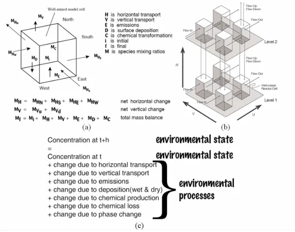
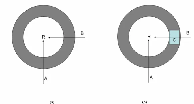
Figure 1.1. Conceptual representation of environmental processes in a typical air quality model: (a) presents the process dynamics in a virtual cell represented as a continuous stirred tank reactor, (b) displays the interaction of each cell with its
neighbor cells, (c) describes the time marching scheme used in solving PDEs (Jeffries, 1995a). ... 5
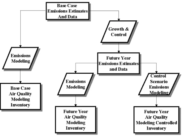
Figure 1.2. Emission inventories needed for State Implementation Plan modeling... 9
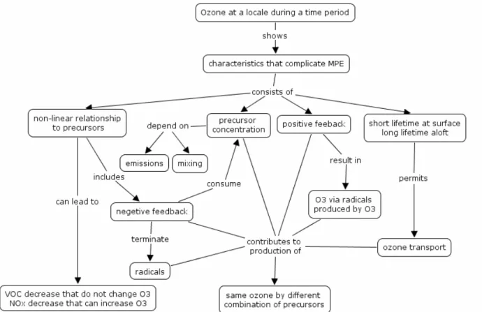
Figure 2.1. A conceptual map of some ozone characteristics that makes MPE difficult. ... 25
Figure 2.2. A conceptual map of SIP modeling and the role of MPE. Shadowed boxes with bold fonts represent concepts that PROMPT includes as primary materials; Traditional MPE approaches were weak in incorporating these. The number in ovals indicates two major modeling steps in SIP modeling: (1) base case modeling and (2) future (and future control) case modeling. ... 27
Figure 2.3. An example bar chart showing daily peak ozone. Data used for this chart is from Houston-Galveston Mid-Course Review 1993 modeling case and all monitors are sorted by its location from west to east with observed ozone and model predicted ozone. As shown in the figure, there are large spatial discrepancies in peak ozone in model and real world at monitor sites. Even with these differences, this specific
modeling case could pass EPA’s three statistical tests. ... 51
Figure 2.4. Illustrative examples of wind scatter plots (top), wind time series plot (bottom left), and wind error time series plot (bottom right) at a monitor site. In these plots, times of a day are encoded with different markers and colors. Model prediction and observation are in different colors. This specific case shows gross (> 60 degree) wind direction differences between modeled winds and observed winds from 1300 to 1700. A series of questions should be asked and answered to investigate if these
discrepancies will affect control strategy developments. ...56
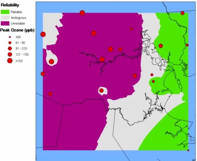
Figure 2.6. Example outcome of PI-P4. Areas are color-coded by an evaluator’s confidence on a model performance. The red circles represent the peak ozone
observed at monitor sites and values in legends for ozone are in ppb... 69
Figure 3.1. Overview of pyPASS operation. Box 1 depicts the general pyPASS operation necessary once for an episode. Box 2 represents the general pyPASS operation needed for each simulation. Once a simulation is performed for an episode, users may run multiple pyPASS operations with visualization modules and package materials for subsequent analyses and communication with documentation modules... 98
Figure 3.2. An example of spatially paired and temporally unpaired daily peak ozone bar chart. The predicted ozone data were made by TCEQ’s HGMCR modeling with CAMx (red) and University of Houston’s modeling with CMAQ (blue) for 2000-08-25. Monitoring sites are sorted by location from west to east of HGMCR modeling domain. The x-axis label denotes the four-letter site codes and the y-axis shows ozone concentration along with one-hour ozone NAAQS (depicted as the purple line) with the label ‘Exceedance’. ...106
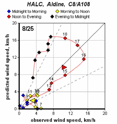
Figure 3.3. Example of a wind speed scatter plot at a single site. X-axis is the
observed wind speeds and Y-axis is the predicted wind speeds in units that reflect the size of the model grids (e.g. 4 km on each side). The magenta spline curve is to help modelers track each data point sequentially. Daylight hours are numbered in LST. Diagonal lines represent 2:1 (dotted), 1:1 (solid), and 1:2 (dotted), correspondence between predictions and observations. Four different colors are used to distinguish four time periods of a day: 0000-0600 (“Midnight to Morning”), 0700-1200
(“Morning to Noon”), 1300-1800 (“Noon to Evening”), and 1900-2400 (“Evening to Midnight”). Left facing and right facing triangles represent pairs of the observed and modeled vector resultant wind speeds in the morning and afternoon... 109
Figure 3.4. An example of graphical measures for surface wind analyses: (a) hodograms (i.e. wind time series plots) and (b) wind error time series plots. For hodograms, the origin is the station locations, the radial axis shows wind speed in km/h, and the angular axis shows wind direction in degrees with 0 degrees as winds from north. Each filled circle is the start point of a wind vector with its arrow head at the origin where the station is located (the vectors are not drawn, but the “tails” are connected by a colored line). Magenta is for observations and cyan is for predictions. Triangles are for resultant winds; left-facing one is for morning and right-facing one is for afternoon. Some hours of day data points are labeled with its hour of day such as “13”. For wind error plots, the radial axis is the ratio of modeled wind speeds to observed wind speeds on a log scale. The angular axis is the degree of wind directional differences between predictions and observations. The green circle is a ratio of 1.0 or when observed wind speeds are same as predicted wind speeds. In an ideal case, all points are located at the cross point of 0 degree line and the green circle. ... 111
with different colors. This plot clarifies when the large underestimation of NO that can be found in scatter plots occurred during the early morning. It is clear that there was also a large ozone underestimation for 1200-1600... 113
Figure 3.6. Example of pyPASS tile plot. This type of tile plots is unique pyPASS outputs that are not available by existing tools. Bottom X-axis and left Y-axis are for x and y coordinates in projected coordinate system. Top X-axis and right Y-axis are for cell coordinates. These axes are optional and users can produce a tile plot without these auxiliary axes, if necessary. All monitors are represented as diamonds filled with different colors depending on the observed ozone concentrations and arrows that has a length equal to the distance of wind traveled for an hour. If there is no observed wind and no chemical measurement, diamonds are replaced with two different sizes of circles superimposed. If there is no observed wind at a monitor, an arrow is replaced with a circle. If there is no measured chemical concentration at a monitor, the diamond is replaced with a circle. The tile plot also holds important geographical features such as highways and coastal lines. Predicted winds are drawn with light
grey arrows... 115 Figure 3.7. Series of tile plots for O3 with predicted surface winds as well as
observed winds and ozone. All time in this plot is hours of 2000-08-25 in LST. ... 117
Figure 3.8. An example pyPASS application to GIS maps. This example is the result of overlaying Figure 3.4 (a) on a GIS map containing important emission sources (normal triangles) and monitors (squares with four-letter site codes). Other
geographical features included in this figure are area sources such as airports (gray
filled polygons), major roads (light brown and yellow), water bodies (sky blue)... 119
Figure 3.9. Example of comparison of aircraft observation with model predictions. The top plot is the pyPASS output for comparing aircraft measurements with model predictions. The bottom plot was made from a GIS map and a part of Flying Data Grabber outputs (McNally, 2005). The black and red arrows in the bottom plot indicate observed winds and predicted winds used for modeling at sampling locations of aircraft flight path. The purple box is the time window corresponding to the purple circle in the bottom map. ... 123
Figure 4.1. Domains for the HGMCR modeling. BPA domain was considered in the early phase of modeling but excluded in the HGMCR modeling. More detailed information such as map projection parameters can be found on TCEQ’s HGMCR
modeling web site (TCEQ, 2006c). ... 141
Figure 4.3. Example package needed for daily graphical performance analyses as part of P1.3 in which a model behavior is compared with the conceptual model. Each package consists of four graphical measures: a bar chart of unpaired peak ozone concentrations (first from top), a bar chart of unpaired maximum hourly ozone changes (second), a bar chart of unpaired peak NO (third) and NO2 (last). The X-axis of each bar chart shows monitors sorted from east to west. Model data were
depicted in red in bar charts. ... 152
Figure 4.4. Example package needed for site-by-site and day-by-day graphical performance analyses as part of P1.3. Each package consists of two graphical measures: surface wind speed scatter plots (left), and time series plots (right). For detailed guidance on how to use each graphical measure, refer to the pyPASS article (Kim and Jeffries, 2006c) and to a partial implementation of PROMPT for this case (Jeffries et al., 2005). In the wind speed scatter plots, yellow right-facing triangle and red left-facing triangle represent morning resultant wind speed (RWS) and afternoon RWS. Model data were depicted with dotted lines in time series plots... 153
Figure 4.5. Example package needed for graphical performance analyses required by P2.2. Each package consists of a set of graphical measures: wind speed scatter plots (top), hodogram (bottom left), and wind error plots (bottom right). This example represents one of the worst cases. For example, observed wind speeds were invariant and close to 4 km/h from 1100 to 1300 while predicted wind speeds changed from 4 km/h to 12 km/h. The afternoon wind speeds were mostly twice as fast as observed wind speeds... 160 Figure 4.6. Example package needed for graphical performance analyses required by P2.3. Each package consists of a set of graphical measures: a time series (top left)
and scatter plots for NO, NO2, and O3... 162
Figure 4.7. Example graphical measures used for P2.4: CO at WILT (top), ETH and OLE at C35C (middle and bottom)... 164
Figure 4.8. Comparison of Psito2n2 and RegEvnt1 for ETH (top) as well as O3, NO, and NO2 (bottom) at C35C. The fine dotted lines are for Pisto2n2. The dashed lines are for Regevent1. Observational data are depicted with solid lines with filled
squares... 171
Figure 4.10. Example of graphical analyses for P3.2. Wind time series plot for H08H (top left) and for H03H (top right) overlaid on GIS map. The observed winds are in magenta and the predicted winds are in cyan. The O3, NO, and NO2 time series at LAPT are shown at the bottom. ... 174
Figure 4.11. Ozone concentrations of RegEvnt1 from 1400 to 1500 on 2000-08-30 at the 9th layer. The dots flowing diagonally at lower left corner of tile plots are an aircraft track from 1451 to 1453. Black squares are cells of very high concentrations (> 180 ppb) of ozone. Each tile represents 1 km by 1km grid cells. The estimated
ozone plume width is approximately 6 km. ... 176 Figure 4.12. Ozone concentration predicted by three models at 1500 on 2000-08-30: Psito2n2 ran at 4 km (left), Psito2n2 ran at 1 km (middle), RegEvnt1 at 1 km (right). . 178
Figure 4.13. Results of statistical performance tests of Psito2n2 and RegEvnt1 for 2000-08-30. All of statistical measures were estimated for each monitoring site using the equations proposed by EPA (US EPA, 1991)... 182
1. INTRODUCTION
1.1 Background
The Clean Air Act (CAA) names “criteria” pollutants that must be regulated due to
public health and welfare concerns. The criteria pollutants are carbon monoxide, nitrogen
dioxide, ozone, lead, PM2.5 and PM10 (particulate matter < 10 micrometers), and sulfur
dioxide. The CAA requires the Environmental Protection Agency (EPA) to set National
Ambient Air Quality Standards (NAAQS) for these six principal pollutants. There are two
types of NAAQS, primary standards for public health and secondary standards for welfare.
If an area in a state violates any of the primary standards, that area is classified as a
non-attainment area. Each state having a non-non-attainment area is required to develop a State
Implementation Plan (SIP) to reduce each pollutant that exceeds the standard to levels equal
to or below the NAAQS for that area. The primary standard for ozone was a daily maximum
one-hour average of 0.12 ppm (parts per million). Those states in violation of this standard
in one or more areas are required to develop a SIP for ozone reduction and to perform a
model-based attainment demonstration to show that the proposed plan is “more likely than
not” effective in producing attainment at a future date.
Photochemical ozone results from the chain reactions of two important precursors,
nitrogen oxides (NOX) and volatile organic compounds (VOCs), in the troposphere with
intense sunlight (Jeffries, 1995a). NO and a small amount of NO2 are created by virtually all
combustion processes because air is used as an oxidant, and high temperature (over
NO will be oxidized into NO2 quickly by ozone and other oxygenated radicals. This is why
NOX, the sum of NOand NO2, is often considered to be the actual precursor to ozone.
VOCs will also undergo a series of oxidation processes that depend on the reactivity of each
VOC with OH· radicals and ozone. Even though ozone is formed during this series of
oxidation processes, none of the atoms in the precursors end up in the ozone molecules.
Ozone is formed by the reaction of O2 and O(3P) that is released from the photolysis of NO2.
TheNO2 molecules are formed in the process of NO oxidation by ozone or peroxy radicals
such as RO2· and HO2·. These peroxy radicals are created in the oxidation process of VOCs
byOH· radicals. OH· radicals are recycled and new OH·radicals are created throughout
photochemical reaction systems by photolytic processes of oxygenated organic compounds
and ozone (Jeffries and Tonnesen, 1994). Ozone formation is complex because of the
feedback of recycled radicals and the fact that a major species in the radical propagation
chain can also serve as a radical terminator.
The control of photochemical ozone is essentially a matter of reducing one or both of
the two major precursors, NOX and VOCs. However, reductions of a precursor do not
always lead to the reduction of ozone. A specific control strategy becomes a complex
problem because there are various sources of NOX and VOCs in non-attainment areas and
their emissions vary in space and time. Moreover, controls of some sources are beyond a
state’s authority. Two examples are: (1) automobiles on interstate highways are major NOx
sources, but their emissions are under the control of the federal government, and (2) trees are
large sources of biogenic hydrocarbons but can not be “regulated” under the CAA. Besides
issues related to ozone chemistry and meteorology: non-linearity of ozone formation and
ozone transport.
The non-linearity of ozone formation results from positive and negative feedback
characteristics of ozone chemistry. Depending on the environment, a reduction of NOX or
VOCs may achieve a small reduction of ozone or produce more ozone. Also, reductions of
both precursors may not lead to the same proportional reduction of ozone even though it will
not cause more ozone formation. This nonlinearity can also result in the same ozone
concentration being produced by different precursor conditions. Thus, linear control of
precursors will not guarantee the desired ozone reduction. While the non-linearity is likely a
local chemistry issue, ozone transport is the phenomenon that ozone and precursors are
carried from upwind areas to downwind areas. As a consequence, a local control strategy
alone may not be sufficient to meet the NAAQS in some cases and this phenomenon
sometimes results in multi-state problems (Farrell and Keating, 2002). Due to these
complexities of the ozone control problem, the CAA Amendments of 1990 require any state
preparing a SIP for future ozone attainment to demonstrate the effectiveness of the control
strategy by using a three dimensional photochemical air quality model (PAQM) or an
equivalent analysis tool.
1.2 Air quality modeling
To simulate ozone formation, a PAQM must have adequate representations of several
environmental processes. Modern PAQMs represent not only gas-phase chemistry but also
horizontal advection and diffusion, vertical advection and diffusion, wet/dry deposition,
these processes are translated into a mathematical expression: a set of nonlinear partial
differential equations (PDEs) such as,
i i i T i i S R C D C U t C w w ) ( )
( ; (1)
whereCi is the mean concentration of species i,U is the mean wind vector; DT is the
turbulent diffusion coefficient; Ri is the removal rate that includes wet/dry deposition rate and
chemistry loss rate; Si is the source term that includes chemistry production rate and emission
rate.
Because this original set of mathematical problems can not be solved analytically,
solutions are usually obtained by numerical methods. As illustrated in Figure 1.1, the most
frequently used numerical methods in PAQMs are formulated on the concept of a collection
of “well-mixed boxes” for spatial integration and the concept of time marching for temporal
In each box in a model, the chemical transformation is estimated. Even a semi-explicit
representation of complex chemistry would require the modeling of thousands of reactions
involving hundreds of species. The equation for this chemistry is known as a “stiff” problem
and leads to high computational costs. Moreover, not all reaction rate constants are known
and the chemistry of some species has not been studied sufficiently. Therefore, PAQM
developers often design compressed or approximate chemical mechanisms to balance the
computational burden against details of the current best atmospheric chemistry knowledge.
In general, virtually all important inorganic species are explicitly represented in these
compressed chemical mechanisms while most VOCs are classified based on their
structure-reactivity relationship or grouped into a few model species (Dodge, 2000).
The most widely used chemical mechanism in PAQMs is the Carbon Bond IV (CB4)
mechanism that consists of about a hundred reactions of approximately 40 model species
(Dodge, 2000). The limitation of this approach includes model compounds that cannot be
directly compared with measured real species. For example, PAR in CB4 represents
saturated hydrocarbon bonding (C-C) and many real species contribute to the concentration
ofPAR in the model.
The operation of a PAQM requires some inputs from other models or observations
(Russell and Dennis, 2000). The two most important types of models that provide PAQM
inputs are the meteorological models and the emissions models. Meteorological inputs
include wind fields, surface temperature, and other parameters. Some of these are also used
to generate emission inputs because some emissions depend on meteorological conditions.
For example, biogenic emissions depend on ambient air temperature. Emission inputs are
requires LULC information and the meteorological model uses LULC information for its
surface roughness estimation.
Each auxiliary model that generates PAQM inputs is, by itself, a complex model that is
subject to a performance evaluation and quality assurance/quality controls (QA/QC). As a
consequence of this operational complexity, interdisciplinary team efforts and comprehensive
knowledge are required to exercise the PAQM effectively and to use the modeling results
appropriately in the decision making process.
1.3 Model performance evaluation
The judgment of the quality of the modeling results is important. The results of SIP
modeling are intended to inform policy decisions regarding the control of high ozone in
non-attainment areas. Some of those decisions will be implemented as part of the SIP and may
result in the placement of large burdens on social resources and significant influences on
daily life, e.g., restriction of construction hours, changes in speed limits, or extra automobile
fees. The PAQM performance evaluation is to assess the quality of the modeling results used
in decision making processes. The PAQM performance evaluation for SIP modeling is
different from the PAQM evaluation for scientific research that examines the correctness of
the PAQM formulation and tests whether a PAQM is generally operational (Russell and
Dennis, 2000). If the formulation of a PAQM is generally acceptable to the air quality
modeling community or it is peer-reviewed by the EPA, the PAQM is classified as an
operational PAQM.
In general, the PAQM evaluation for scientific research is not part of the SIP application
because it requires well-designed field studies and intensive evaluations. For a SIP
PAQM to determine its suitability for use in the SIP development. Upon the EPA’s approval,
the state uses the PAQM as its SIP development tool.
For a SIP development, a state completes a series of steps. The state attempts to
reproduce high ozone concentrations over non-attainment areas with episodic meteorology
and historic emissions using the selected PAQM. This modeling case is known as the “base
case”. If the model performance is considered to be good, the state simulates future ozone
levels with the episodic meteorology and future estimated emissions. The future estimated
emissions are a combination of projected current emissions that include growth and existing
Federal and State regulations already required. The future ozone simulation is known as the
“future case”. If the predicted ozone level is over the NAAQS, the state will need to propose
new control requirements, apply them to the future case emissions, and run the PAQM to test
the effectiveness of the control plans. This modeling case is known as the “future control
case”. Figure 1.2 shows emission inventories needed for a SIP modeling. Often, the ‘future
control case’ is called the ‘future case’ because it is highly unlikely to meet the NAAQS with
just the initial future case involving only Federal level controls. Hereafter, ‘future case’
means ‘future control case’ unless specifically noted. The attainment demonstration is to
show that the non-attainment areas will “more likely than not” be in attainment with the
proposed control plans. During a SIP development, therefore, the PAQM performance
evaluation is a vital process because most policymakers are not willing to make decisions
The PAQM performance evaluation for the SIP application focuses on the matching
history of the PAQM results in a base case modeling and the utility of the PAQM for the SIP
development task in a future case modeling. Since 1991, the EPA has issued three guidance
documents to assist states in operating a PAQM, evaluating a PAQM performance, and using
the modeling results in their attainment demonstration process (US EPA, 1991; US EPA,
1996; US EPA, 1999).
The 1991 EPA guidance for the model performance evaluation mainly focused on how
to determine the pass/fail status of the PAQM performance for the attainment demonstration
purpose. Even though the 1991 EPA guidance contains several measures for the model
performance, in practice, virtually all SIP applications use the most basic measures; unpaired
peak accuracy, bias, and gross error. For details about how to compute these measures, refer
to Table 1.1. Consequently, in spite of the 1991 guidance, the attainment demonstration has
been very difficult for states to conduct as shown in recent experiences in two of the largest
states, Texas and California (Jeffries, 2005). Sometimes, it has even been hard for the EPA
modeling development group to conduct the model performance evaluation properly. For
example, the operational use of the EPA’s newest model, the Models-3/Community
Multi-scale Air Quality modeling system (Models-3/CMAQ), was delayed more than a year even
developed over a decade-long effort because emission inventories were inadequate to
demonstrate that the model could be used to perform SIP modeling with the 1991 guidance
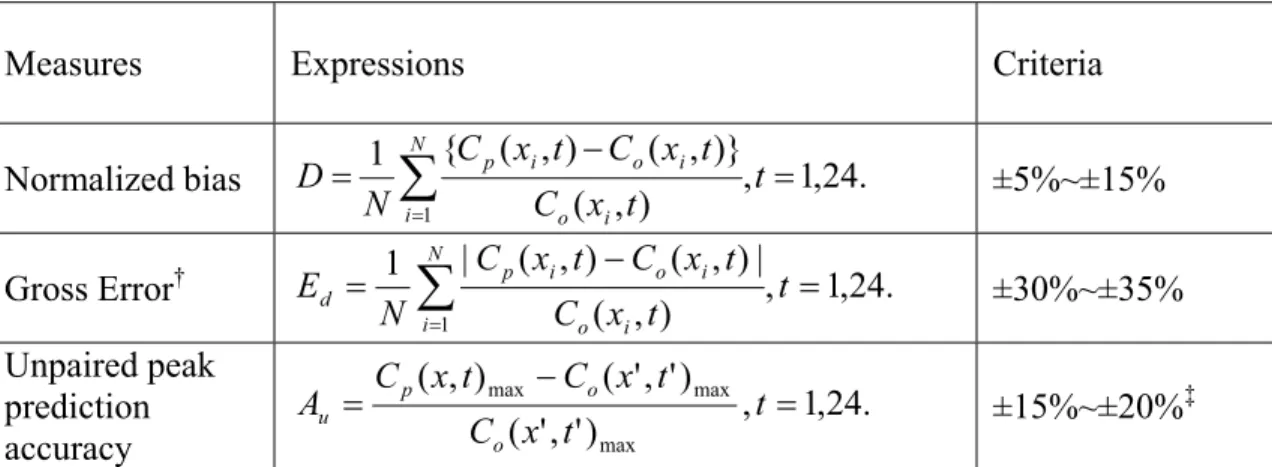
Table 1.1. Most frequently used measures to determine a PAQM performance evaluation in a SIP application.
Measures Expressions Criteria
Normalized bias , 1,24.
) , ( )} , ( ) , ( { 1 1
¦
t t x C t x C t x C N D Ni o i
i o i
p
±5%~±15%
Gross Error† , 1,24.
) , ( | ) , ( ) , ( | 1 1
¦
t t x C t x C t x C N E Ni o i
i o i p d ±30%~±35% Unpaired peak prediction accuracy . 24 , 1 , ) ' , ' ( ) ' , ' ( ) , ( max max max t t x C t x C t x C A o o p u ±15%~±20% ‡
Where N is the number of monitoring stations, CO(xi,t) and CP(xi,t) denote observed and predicted
concentration of ozone at ith monitoring station at time t, respectively. †For hourly observed values of O3 > 60 ppb.
The 1996 guidance provided two approaches for attainment demonstrations: the
Deterministic Approach and the Statistical Approach. The Deterministic Approach was
almost the same as the attainment demonstration requirement in the 1991 guidance, except
that the standard of passing the test is raised from 120 ppb to 124 ppb and the
‘weight-of-evidence’ (WOE) analysis is recommended if the attainment demonstration by a PAQM is
“close enough”. The WOE concept is the tool that EPA offered states to account for the
model uncertainties for the attainment demonstration. The 1996 EPA guidance essentially
attempted to deal with inherited uncertainties in the modeling results by PAQMs available at
that time and problems with estimating future emissions. On the other hand, the Statistical
Approach has not been pursued much. This approach requires more ‘burden of proof’ for its
‘weight-of-evidence’ formulation than the Deterministic Approach, which may explain the
infrequent use of the Statistical Approach.
The 1999 EPA guidance, only four pages in length, provided a way to estimate
additional emission reduction requirements for attainment demonstrations by combining
modeling results and observations to overcome some of the regional transport problems
without doing actual modeling as part of the ‘weight-of-evidence’ arguments. This guidance
was intended to solve a “one time” problem that EPA had in the resolution of a DC Circuit
Court Case, but resulted in SIPs submitted from 13 states (Jeffries, 2005).
Even though EPA made efforts to account for the uncertainties of the modeling results
by ‘weight-of-evidence’ analysis in the 1996 guidance, no specific guidelines or protocols
were given to states about ‘how-to’ do this appropriately. Consequently, current protocols
proposed by many states for SIP modeling only contain the most basic measures introduced
the EPA has the authority to approve modeling protocols and attainment demonstrations
proposed by states. The problem is that the EPA has not established criteria explicitly on
evaluating the results of the WOE analyses. Instead, the EPA has accepted the WOE
arguments on a case-by-case basis. Therefore, the current process of accepting the model
performance is too subjective and sometimes even controversial considering the past decision
the EPA made. For example, the EPA approved a SIP submitted by Georgia that used the
linear rollback approach to fill a large gap of ozone control requirement as part of the WOE
analysis (66 FR 63972, 2001). But the linear rollback approach is a method that the EPA
does not recommend as a major ozone control strategy. Another example of the absurd uses
of WOE analysis for attainment demonstration is New York’s SIP. The model used by the
state predicted peak ozone as high as 171 ppb in its future case, then the state conducted
linear ozone reduction tests as part of the WOE analysis to argue that they can decrease the
peak ozone level in the future as low as 118 ppb, which the Court ruled as acceptable (2nd
Circuit, 2003).
While the model performance evaluation always involves subjective judgments, a model
performance evaluation that lacks good objective analyses can mislead policymakers into
making arbitrary and capricious emission reductions that have nothing to do with ozone
control. Moreover, the legal system interprets the completion of the minimum requirements
in the EPA guidance documents (such as the creation of time series without further analysis)
as satisfying the legal requirement even if the model performance is vague or the modeling
results are wrong due to flawed modeling (5th Circuit, 2003).
In the past, the EPA model performance evaluation practice has focused mainly on the
by using basic statistical measures and graphical measures. It has been noted that this
statistical approach to evaluate overall model performance does not tell much about how a
model gets its answer and it forces a user to accept or reject the modeling results as a whole
(Beck, 2002). This is the obvious weakness of the current EPA’s model performance
evaluation approach because a PAQM may get similar results from different sets of
conditions including different inputs and a PAQM’s partial functionality may be sufficient to
assist decision makers even though a PAQM does not show good overall performance.
It is important to know whether the matching history is obtained via compensating
errors that would preclude the proper use of PAQM results. For example, two different sets
of model inputs (assuming one of the sets is correct) could make the PAQM show similar
matching history performance, for example, one of the model inputs could be lower mixing
heights coupled with less emissions than a second set of inputs but both sets produce
predictions are close. However, the PAQM’s responses to the future scenario from these two
input sets will be different and the policymaking based on one of the input sets will be in
error and may not be effective. The problem is that it is almost impossible to detect
compensating errors by just looking at ozone prediction alone because ozone is a secondary
pollutant. Consequently, the evaluation of the PAQM performance should examine if the
PAQM shows good ‘matching history’ of precursors as well as ozone. Further, the
magnitude of the processes in the model that lead to the critical ozone production that
dominates the decisions should be investigated, visualized and contrasted to similar processes
in other modeling scenarios.
Evaluation of ‘matching history’ of precursors and ozone should also include evaluation
amount of precursors moves in and out of a place at the right time. In the current EPA
performance guidance documents, meteorological inputs are evaluated with meteorological
observations before the PAQM performance evaluation. The meteorological inputs are
generated by a meteorological model outside a PAQM. Also, the actual meteorological
model outputs are modified with special processors to align grids of the meteorological
model to grids of the PAQM. While the meteorological inputs may result in an acceptable
overall performance against the meteorological observation, they may not be acceptable for
ozone prediction at some places for certain times because of less acceptable performance for
mass transport and dilution, which are not evaluated with the typical meteorological
observations. Therefore, it is desirable to evaluate the PAQM performance conditionally
upon the performance of the meteorological inputs. This is not required in the EPA guidance.
Even if a PAQM produces answers free from compensating errors, it is hard to
determine one ‘optimal’ model prediction because some acceptable input sets can result in
very similar ozone prediction and we are not sure which input set is more close to reality due
to our lack of knowledge and uncertainties; critical aspects of our environmental system are
essentially unknowable given current measurement capabilities. Also, given uncertainties in
policymaking other than the modeling uncertainties, it is not necessary to have the “most”
optimized model prediction for good policymaking unless non-optimal model prediction is
very different from the optimal prediction. Rather, it will be more important to examine
whether the PAQM results can provide directionally correct information (e.g. NOx control or
VOCs control), how biased the PAQM results might be, and what the effects of the biases
will be on the policymaking. The evaluation of a PAQM as a tool needs to examine whether
Few research investigations have been done regarding the performance evaluation
conditionally upon the quality of the model inputs and how to evaluate a PAQM with its
performance to fulfill its designed tasks (Roth, 1999; Fine et al., 2003; Roth et al., 2005).
Dramatic increases in computer performance and the widespread use of commercial
off-the-shelf components to create a cheap super-computer such as Beowulf clusters have made it
easy to operate the PAQM repeatedly. While more people can run the models more cheaply
than ever before, no protocol has been developed to guide users in judging the performance
of the PAQM in a more comprehensive way. The lack of timely judgment in using and
evaluating the inputs and operational choices available in the modeling system, coupled with
the failure to integrate the policy components of the problem with the technical modeling
components, have resulted in failed modeling efforts (Keating, 1997). Some of these failed
modeling efforts have required significant legal actions to remedy them (Texas, 2004), while
others have resulted in significant delays in cleaning up the atmosphere and providing a
healthier environment (69 FR 8126, 2004; 69 FR 16483, 2004). For more reliable air quality
management, we need a model performance evaluation protocol that permits users to
examine the PAQM performance conditionally upon the quality of the model inputs and to
assess the PAQM utility for the decision making given biases of the PAQM outputs.
1.4 Goal and objectives
The long term goal of my work is to establish a process that can produce “serviceable
truth” in environmental management depending on modeling studies. By definition,
serviceable truth is “a state of knowledge that satisfies tests of scientific acceptability and
supports reasoned decision-making, but also assures those exposed to risk that their interests
The development of process for serviceable truth will require much broader understanding of
various fields and interdisciplinary efforts in a holistic way. In this study, I only attempt to
resolve issues found in the scientific realm. That is, I focused on how to evaluate
environmental models aptly for supporting decision-makers.
In ozone air quality modeling field, a concept of ‘vindicating the use of PAQMs’
(Jeffries, 1995b) emerged a decade ago. This study is a realization of that notion and can be
considered as a case-study; the framework and notions developed here can be used for
achieving the ultimate goal. My intention was to develop a way of bringing science into
policy decision making processes by using PAQMs appropriately so that modelers help
policy makers avoid arbitrary and capricious decisions under given modeling uncertainties
and resource constraints. MPE is the critical process for using PAQMs appropriately (Roth,
1999; Russell and Dennis, 2000; Roth et al., 2005) and I found there is no good study on this
subject at present.
The specific goal of this study was to develop an alternative protocol to the EPA’s
current performance evaluation protocol and suitable tools that permits thoughtful modelers
to answer the following questions by conducting comprehensive performance analyses
systematically: To what extent can I accept the PAQM predictions at face value for a SIP
development? And if I cannot, then how should I make judgments about the effectiveness of
ozone control options?
These questions cannot be answered by following the EPA’s current protocol without
performing many ad hoc diagnostic analyses. Often, these analyses require a lot of time and
manner. Without good systematic guidance, many of these analyses can be ineffective
because some analyses often turn out to be irrelevant to the given problems.
Three objectives are set to achieve the goal of this study:
1. Formulation of an improved MPE protocol that will help modelers answer ozone
policy relevant questions effectively,
2. Development of computerized tools suitable for implementing the MPE protocol
developed in this study so that modelers can utilize the new MPE method for
real SIP modeling and achieve the goal of MPE in a timely manner, and
3. Application of the new MPE protocol and computerized tools to a real SIP
modeling case to demonstrate that the new MPE method and tools developed in
2. DEVELOPMENT OF AN IMPROVED PROTOCOL FOR
EVALUATING THE PERFORMANCE OF REGULATORY
PHOTOCHEMICAL AIR QUALITY MODELS
Abstract
In the application of photochemical air quality models (PAQMs) for State
Implementation Plan (SIP) development, appropriate model performance evaluation (MPE)
is critical and mandatory. The traditional largely statistical-based MPE protocols must be
often used by state modelers, but those protocols have important disadvantages in generating
useful information for supporting ozone decision-making. These disadvantages include
allowing model users (1) to accept modeling results that may lead to directionally incorrect
emission controls or (2) to reject, as a whole, partially useful modeling results for policy
decisions. In this paper, we introduce the Protocol for Regulatory Ozone Modeling
Performance Tests (PROMPT), a meta-protocol to improve regulatory air quality model
performance evaluation. We derived the underlying principles formulating PROMPT from
discussions appearing in the recent literature, emphasizing graphical evaluations and the
direct assessment of model performance with regard to ozone control policy questions. We
developed the structure and details of PROMPT based on these principles and on our
practical experience with real-world SIP modeling analyses. PROMPT contains four major
sets of procedures that are specifically designed to evaluate the usefulness of models for SIP
development and to provide more explicit information aimed at assisting decision makers
effectively. Each set of procedures is composed of a statement of analysis goal, the required
information for proposed analyses, a list of the core tasks, and the expected outcomes of each
task. Also included are the relationships among different procedures and documentation
specifications about reporting analysis results. We conclude that PROMPT can serve the
regulatory photochemical ozone modeling community better than traditional approaches by
more systematic and comprehensive performance evaluation. PROMPT will result in cleaner
policy-relevant scientific answers to the posed policy questions more directly than the
2.1 Introduction
Ozone is a pure secondary pollutant: it is not emitted directly from sources but is formed
in the atmosphere when two major precursors, NOx (=NO+NO2) and volatile organic
compounds (VOCs), react under conducive ozone formation conditions such as weak winds
and intense sunlight (Jeffries, 1995a). The precursors are released from multiple sources
including industrial facilities, cars, and natural sources like soils and trees. Precursor
emissions are, however, a necessary but not a sufficient condition for ozone formation.
Meteorological factors including winds and mixing heights are important because these
determine the transport and mixing of precursors, and thus, eventually control the
concentration-dependent chemistry that leads to ozone. Certain meteorological conditions
can cause ‘ozone transport’ (OTAG, 1997) that results in multi-state problems (Farrell and
Keating, 2002) in which local controls can become ineffective. Because any effective
intervention requires causal explanations (Pearl, 2000), the ability to explain the causes of
ozone problems at a particular locale is a critical key to finding solutions to prevent
occurrences of similar ozone problems in the future and requires insight into complex
relationships among meteorology, emissions, and chemistry. At the same time, it is
noteworthy that an ozone problem in a locale at a specific time results from very specific
reasons (e.g. the combination of a particular meteorological condition with spatiotemporally
unique emissions). Therefore, it is highly desirable to conduct explanatory studies for more
than one ozone episode to obtain representative insights of causes of any frequent ozone
problems at a locale.
Because eulerian photochemical air quality models (PAQMs) were considered the most
conditions (National Research Council., 1991), the 1990 CAA Amendments (CAAA 1990)
highly recommended the use of PAQMs as the primary investigation tool for regulatory
ozone problems. The CAAA 1990 requires the use of PAQM as a legally-binding apparatus
to seek solutions to a given ozone problem for moderate and above non-attainment areas
(NAAs) to the old 1-hour ozone National Ambient Air Quality Standard (NAAQS), as well
as all of NAAs to the new 8-hour ozone NAAQS (US EPA, 2003). In the use of PAQMs, the
Environmental Protection Agency (EPA) also mandates conducting model performance
evaluation (MPE) following an EPA approved protocol. MPE is the process of gauging the
reliability of PAQMs as tools for testing the effectiveness of possible emission control
options (National Research Council., 1991). Some researchers argued that the new 8-hour
standard is expected to be more difficult to attain than the old 1-hour standard because
violations are likely to extend to rural areas from urban areas (Chameides et al., 1997).
Therefore, it is not hard to imagine that the operation, evaluation, and application of PAQMs
will be more complicated, difficult, and resource-demanding in meeting the new 8-hour
standards.
The correct identification of causes of ozone problems in terms of precursor
contributions is especially important in the MPE of PAQMs. As shown in Figure 2.1,
however, MPE of PAQMs becomes a very difficult task because the ozone formation
mechanism includes positive and negative feedback processes. These two-way feedback
processes result in the nonlinearity of ozone formation, e.g. that excessive NOx can inhibit
ozone formation and some VOC reduction may have no effect. Therefore, when the
condition of a locale is NOx-rich, NOx emission controls can result in increased ozone
toNOx control from the response of real world ozone, then this type of flawed modeling can
result in directionally incorrect control recommendations such as irrelevant NOx control
whenVOC control is necessary. Failure to conduct a proper MPE can lead technical staffs
in state agencies to provide wrong information to the policy makers. A consequence of
misleading policy makers could be serious given that (1) the compliance cost for ozone is
over a billion US dollars (US EPA, 1997), (2) more than 100 million people in the United
States live in areas of poor ozone air quality as of 2003 (US EPA, 2004), and (3) ozone still
remains the most persistent air pollutant in the United States even after more than two
decades of control strategy developments and implementations to solve ozone problems
(OTA, 1989; National Research Council., 1991; Georgopoulos, 1995; US EPA, 2004).
Improving MPE methods has been one of the most difficult research areas in the
photochemical air quality modeling community (National Research Council., 1991;
Georgopoulos, 1995; Russell and Dennis, 2000; Fine et al., 2003), especially for MPE
methods suitable for a peer-review conducted by a third-party of a regulatory PAQM
application (Roth, 1999). The purpose of this paper is to introduce the Protocol for
Regulatory Ozone Modeling Performance Tests (PROMPT) which is a meta-protocol that
state SIP modelers and third-party model evaluators can utilize as a guideline MPE protocol
to develop their own specific MPE protocol. This process will subsume and improve the
2.2 Review of SIP modeling and MPE practice
Figure 2.2 conceptualizes how SIP modeling is initiated and conducted. Also this figure
shows who the major players are in the process and what components are involved in the
whole process. This figure should be consulted for the rest of this paper as a road map for
the SIP modeling process. The shadowed boxes in Figure 2.2 represent concepts that we
adopt or enhance in our PROMPT development.
2.2.1 SIP modeling
In this section, we discuss the SIP modeling process (refer to Figure 2.2 as the map of
this section). A state with an area in violation of the NAAQS must develop and submit a SIP
that includes a future attainment demonstration; this much be done before the statutory
deadline. Otherwise, the state might face sanctions or EPA may impose a Federal
Implementation Plan. ‘SIP modeling’ is the modeling process that a state undertakes for the
attainment demonstration in the SIP. Before conducting ozone SIP modeling, the state
selects one or more PAQM(s) and at least one ozone NAAQS violation historic episode. The
model and episode selections are subject to EPA’s approval. Once approved, the state
conducts a series of three major modeling tasks with each meteorological condition of the
27
ap of SIP m
odeling
and the role of MPE. Sha
dowed boxes w
ith bold fonts represent concepts that
rim
ary m
aterials; T
raditio
nal MPE ap
proaches were weak in incorporating these. The num
ber in ovals
ajor m
o
deling steps in SIP m
odeling: (1) base case m
odeling and (2) future (and future control) case m
ode
The first major modeling task is ‘base case’ modeling (shown in the box marked with an
oval of ‘1’ in Figure 2.2) that attempts to replicate an historic ozone episode using adjusted
historic emissions and simulated meteorological fields for the time period of the episode. If
the base case is acceptable, the second major modeling task is to simulate a ‘future case’
(shown in the box marked with an oval of ‘2’ in Figure 2.2) that predicts the future ozone
statewith the base case meteorology and with projected emissions based on controls that are
already “on the books” such as existing ‘Rate-Of-Progress’ and on federal programs such as
mobile source controls. Note that modifying mobile source controls is not available as a
control option to the state; i.e. they are prescribed by US EPA. If the ‘future case’ does not
show attainment with these mandatory controls, the third major modeling task is to create a
‘future control case’ (also shown in the box marked with an oval ‘2’ in Figure 2.2) that
simulates effects of any additional controls needed for the ‘future case’ to show attainment.
These controls come from the ‘catalog’ of controls suggested by policymakers. Frequently, a
simple future case, without additional controls, does not show attainment (Russell and
Dennis, 2000), thus, a ‘future control case’ is often considered as the real ‘future case’.
Hereafter, the term ‘future case’ means the ‘future control case’ unless otherwise be noted.
From this description, we can find two important characteristics of SIP modeling. First,
SIP modeling is constrained by a policy timeline and framework. Typical modeling done for
scientific purposes is rarely constrained by such external factors. Second, we recognize that
all future cases in the SIP modeling can be thought of as merely sensitivity test cases of the
base case because the base case meteorology is used for all future cases and the future
emissions are projected from the base case emissions. Thus, we see that the quality of future
quality of base case modeling. This point is often misunderstood by policy makers, and even
some state modelers (Smith, 2004b). Note that the new 8 hour modeling may introduce a
breakage in the consistency between the base case emissions and the future case emissions by
adopting ‘base line’ emissions. For details, refer to the EPA’s 8 hour modeling guideline
(US EPA, 2005b). At this point, we do not know yet how to resolve this inconsistency in
emission estimations with respect to proper model evaluations.
2.2.2 MPE practice
For PAQM evaluation in regulatory applications, EPA has developed a series of
modeling guidance documents (US EPA, 1991; US EPA, 1996; US EPA, 1999; US EPA,
2005b). These documents contain the recommended measures for the MPE, the criteria of
the MPE, and the criteria for demonstrating attainment. The guidance documents also
recommend performing corroborative analyses and graphical tests along with the three
necessary ‘statistical tests’: normalized bias, gross error, and unpaired peak prediction
accuracy (for a detailed description of how to compute the test statistics, see US EPA, 1991).
In addition to these deterministic evaluations, EPA has more recently developed the
‘weight-of-evidence’ (WOE) determination (US EPA, 1996) as a corroborative analysis for judging
the possibility of attainment under modeling uncertainties when the future case is close to
attainment. For the new 8-hr standards, EPA introduced the ‘relative reduction factor (RRF)’
and some additional statistical measures (US EPA, 2005b) for attainment demonstrations as a
supposedly improved way of accounting for potential uncertainties of PAQM results. As the
modeling community is still gaining experience with these new guidelines, these latter
approaches and measures will not be discussed here.
no clear guidance on what to consider or how to judge acceptance; the guidance merely states
a requirement of making graphs and of conducting general analyses. We agree that MPE is
indeed a human intellectual activity that should involve many subjective judgments. We
insist, however, that there must be rational criteria for these judgments. The description for
how to do a WOE determination is not clear and has been questioned in comments submitted
to EPA on SIPs proposed for acceptance. It is not surprising that most of the PAQM
applications in SIPs only follow EPA’s MPE approach in a very limited way (ENVIRON et
al., 2002; TCEQ, 2004). For example, the three statistical tests proposed in the 1991
guidance document were the primary procedures used in many recent SIPs, even though
other analyses (including graphical analyses) were also recommended in the guidance. The
statistical test criteria for the EPA’s MPE were derived from model performance practice
prior to 1990 (Tesche et al., 1990; US EPA, 1991). These criteria are still used, however, to
judge the performance of modern PAQMs and interestingly there is little difference between
the performance of old models and that of new ones (Russell and Dennis, 2000).
2.2.3 The Courts’ view on the role of MPE
The over use of summary statistics may be in part due to the US Appeals Court’s view
on the guidance documents and EPA’s recommendations (5th Circuit, 2003). As discussed
in the previous section, the statistical performance criteria were provided as guidance or as
suggested performance goals. The legal power of these criteria, however, is beyond that of
suggestion. Following are illustrative examples showing how the US Appeals Courts view
MPE differently from scientists.
The recent US Appeals Court rulings make it legitimate to accept SIPs if states literally
explicitly because EPA required time series creation but did not enforce explicit assessment
of the analysis of time series. Moreover, EPA approved a WOE determination based on the
reduction of 53 ppb from the PAQM predicted 171 ppb peak ozone in the future without
performing any serious analysis of air quality modeling with PAQMs and this was acceptable
to the Appeals Court (2nd Circuit, 2003). Given the fact that ozone formation is highly
non-linear and 171 ppb is not in the range of concentration we can find in our ambient air
routinely, a 53 ppb reduction from 171 ppb may end up being an unnecessary extra emission
control that may not be defensible scientifically. Part of the reason that the Appeals Courts
accepted this weak analysis for the major component of the attainment demonstration is: (1)
the Appeals Court’s view that ‘the reviewing court must remember that the agency is making
predictions at the frontiers of science.’ (2nd Circuit, 2003) and (2) EPA considers a WOE
analysis based on the linear rollback approach (e.g. see 66 FR 63972, 2001) no matter how
high modeled ozone concentrations are as long as PAQM predicted ozone values are starting
points of the linear rollback approach.
2.2.4 Review of selected studies on improving MPE
While there were lawsuits and conflicts in the regulatory arena regarding applications of
MPE and the proper use of PAQMs for decision making, most state modeling staffs and
some in the air quality modeling research community have merely followed EPA’s guidance
as part of research methods without challenging the current MPE practice (Russell and
Dennis, 2000). At the same time, others in the scientific community have recognized that the
current practice of MPE was not sufficient in part because statistical tests should not be the
sole basis for model performance judgment (Willmott, 1984; Tesche et al., 1990).
performance issues within a probabilistic framework (Hanna and Davis, 2002) and studies on
improving MPE with different performance evaluation methods other than the traditional
statistical tests (Hogrefe et al., 2001; Sistla et al., 2001; Fuentes et al., 2003; Sampson and
Guttorp, 1999). The number of studies is small and the studies still contain significant
shortcomings for use in regulatory applications. These will be examined in more detail
below.
Some have argued that approaches utilizing a probabilistic framework is consistent with
the current EPA’s efforts to incorporate the modeling uncertainties in using PAQM results
and to judge the attainment demonstration with RRF and WOE determination (Hanna et al.,
2001). The old 1-hour NAAQS and the new 8-hour NAAQS, however, are set as a ‘bright
line’; that is, the standard only allows rounding-off error as a quantitative uncertainty
tolerance in an attainment demonstration. For example, the NAAQS for 1-hour ozone is 0.12
ppm so that 124 ppb meets NAAQS while 125 ppb does not (US EPA, 1996). In other words,
the current SIP modeling framework does not explicitly allow a formal probabilistic
evaluation in the attainment demonstration. As we noted in the previous section, it is
important to keep in mind that regulatory modeling is constrained by the statutory framework
to which it belongs.
Even though approaches attempting different evaluation methods have potential
advantages over the traditional practice, such alternative approaches are still not mature and
they share some common problems with the traditional approach. For example, some
suggested alternative methods used a performance measure such as the coefficient of
determination, R2, (Sistla et al., 2001), which is often considered inappropriate for the
McCabe Jr., 1999). Some proposed approaches are geostatistical methods (Fuentes et al.,
2003; Sampson and Guttorp, 1999) including mapping technologies, which are considered
impractical for routine evaluation without ample monitored data because of the spatial and
temporal scale issues of ozone formation (Diem, 2003).
The newer formal uncertainty studies (Hanna and Davis, 2002), time series
decomposition studies (Hogrefe et al., 2001), and new evaluation measure studies (Taylor,
2001; Legates and McCabe Jr., 1999), all still exhibit a problem commonly found in
traditional MPE practices: they focus on how to better conduct MPE specifically for ‘ozone
performance’ but ignore the fact that the same ozone concentration can result from many
different combinations of precursor concentrations. Thus they permit “getting the right
answer for the wrong reason”.
This phenomena - getting similarly good answers for different reasons - is called
‘equifinality’ (Beven, 2002), and is one of the general attributes of any environmental model.
Nevertheless, the excessive emphasis on final state variable evaluation is not just a problem
of regulatory photochemical modeling community. Most of the MPE practice in other
application fields also focuses on measuring the matching history of target outcomes with
summary statistics such as mean bias, which does not provide insights into model
performance, and admits apparently good modeling performance that actually arose due to
compensating error or non-linear relationship among products and precursors. This issue
may stem from an outdated and narrow view of the concept of MPE.
2.3 Development of PROMPT
2.3.1 Rethinking MPE for SIP modeling
2001), even though the term, ‘evaluation’, is still mixed with other terms such as ‘validation’
(Roache, 1998) or ‘quality assurance’ (Canepa, 2002). The most succinct expression of the
expected outcomes of a MPE in an environmental modeling application can be summarized
by answering the following three questions (modified from the original questions in Beck,
2002):
x Is the formulation of a model scientifically acceptable in general? (i.e. what is the
adequacy and quality of model formulation for this use?)
x Does a model replicate the observations adequately? (i.e. does it make predictions
that match history?)
x Is a model usable for answering specific (e.g. policy) questions? (i.e. does the model
fulfill the designed task?)
The first MPE outcome question also includes two corollary questions: (1) is the science
encoded in the model ‘sound’ (Crawford-Brown, 2005) and working? (2) Is the
implementation of scientific knowledge achieved through properly applying modeling
procedures of generalization, distortion, and deletion (GDD) to the more complex reality? In
SIP modeling cases, the first question can be answered when a specific PAQM is selected for
a study. In general, a state cannot ‘just pick’ a PAQM. EPA must issue an approval of a
particular PAQM and the approval process requires a state agency to show that a candidate
PAQM is as reliable as one of the PAQMs that EPA has used or one of those that has been
through an evaluation process by another state. Ironically, this very specific reason was part
of the arguments that the California made for its choice of the Comprehensive Air Quality
Model with eXtensions (CAMx) (ENVIRON et al., 2002) over the US EPA’s own