MARGINALLY-SPECIFIED MEAN MODELS FOR COUNTS WITH MIXTURE DISTRIBUTIONS
Habtamu Kassa Benecha
A dissertation submitted to the faculty of the University of North Carolina at Chapel Hill in partial fulllment of the requirements for the degree of Doctor of Philosophy in the
Department of Biostatistics in the Gillings School of Global Public Health.
Chapel Hill 2016
Approved by:
c O 2016
ABSTRACT
Habtamu Kassa Benecha: Marginally-specied Mean Models for Counts with Mixture Distributions
(Under the direction of John Preisser)
ACKNOWLEDGMENTS
The greatest thanks go to my advisor Dr. John Preisser for his guidance and constant support in my research endeavors. I am very grateful for his insight, encouragement, pa-tience, and for helping me grow as a biostatistician. I truly feel fortunate to have had the chance to work closely with him. I would also like to thank Dr. Amy Herring for her support in my research and for her invaluable contributions to my progress from my rst year at UNC all the way through the completion of this dissertation.
Furthermore, I want to thank Drs. Brian Neelon, Kimon Divaris, Donglin Zeng and Kalyan Das for their insightful comments and their time. Special thanks go to Dr. Chirayath Suchindran for his encouragement, advice and support. I would also like to thank Dr. Lloyd Edwards for his mentorship and support, particularly during my rst two years at UNC. Furthermore, I would like to thank Melissa Hobgood and the students, sta and faculty of the Department of Biostatistics for all the help I have received. Thanks also to the National Institute of Environmental Health Sciences and the Gary G. Koch Scholars Program for their nancial support.
TABLE OF CONTENTS
LIST OF TABLES . . . ix
LIST OF FIGURES . . . xi
CHAPTER 1: LITERATURE REVIEW . . . 1
1.1 Introduction . . . 1
1.2 Mixture Models . . . 4
1.2.1 Poisson and Negative Binomial Mixtures . . . 5
1.3 Analysis of Zero-inated Counts . . . 6
1.3.1 ZIP and ZINB Regression Models . . . 7
1.4 Models for Bivariate Zero-inated Counts . . . 9
1.5 Inference About the Overall Population . . . 11
1.5.1 Estimation Based on Latent Coecients . . . 12
1.5.2 Marginalized Models . . . 14
1.6 Missing Data . . . 15
1.6.1 EM Algorithm and Monte Carlo EM Methods . . . 16
CHAPTER 2: MARGINALIZED MIXTURE MODELS FOR COUNT DATA FROM MULTIPLE SOURCE POPULATIONS . . . 20
2.1 Introduction . . . 20
2.2 Models for Zero-inated Data . . . 22
2.2.1 Zero-inated Poisson and Negative Binomial Models . . . 22
2.2.2 Marginalized ZIP and ZINB Models . . . 24
2.3 Finite Mixture Models . . . 25
2.4.1 Models . . . 26
2.4.2 Estimation . . . 29
2.4.3 Algorithm for Finding Starting Values of Parameters . . . 29
2.5 Simulation Study . . . 32
2.6 Application to a Caries Incidence Trial . . . 34
2.7 Discussion . . . 36
CHAPTER 3: MARGINALIZED BIVARIATE ZERO-INFLATED POISSON REGRESSION . . . 46
3.1 Introduction . . . 46
3.2 Zero-inated Bivariate Poisson Models . . . 48
3.3 Marginalized Zero-inated Bivariate Poisson Models . . . 51
3.4 Simulation Study . . . 52
3.5 Application to a School-based Fluoride Mouthrinse Program . . . 55
3.6 Discussion . . . 58
CHAPTER 4: MARGINALIZED ZERO-INFLATED POISSON MODELS WITH MISSING COVARIATES . . . 67
4.1 Introduction . . . 67
4.2 Zero-inated Poisson Models . . . 69
4.3 Marginalized ZIP Models . . . 71
4.4 Monte-Carlo EM for Missing Covariates . . . 72
4.5 Simulation Studies . . . 76
4.6 Application to a School-based Fluoride Mouthrinse Program . . . 78
4.7 Discussion . . . 82
CHAPTER 5: CONCLUSION . . . 88
LIST OF TABLES
2.1 Percent relative median biases of estimates of β1,
β2 and β3 from marginalized mixture models tted
to data generated from the MPois-Pois model with
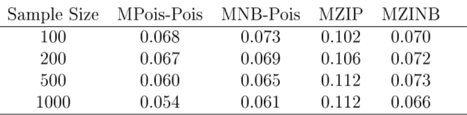
10,000 replications. . . 38 2.2 Type I error rates for the estimate ofβ1from
marginal-ized models tted to data generated from the
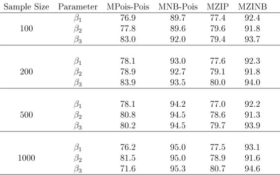
MPois-Pois model with 10,000 replications. . . 39 2.3 Coverages of 95% condence intervals for estimates
of β1, β2 and β3 from marginalized models tted
to data generated from the MPois-Pois model with
10,000 replications. . . 39 2.4 Percentages of converged marginalized models tted
to data generated from the MPois-Pois model with
10,000 replications. . . 40 2.5 Percent relative median biases of estimates of β1,
β2 and β3 from marginalized mixture models tted
to data generated from the MNB-Pois model with
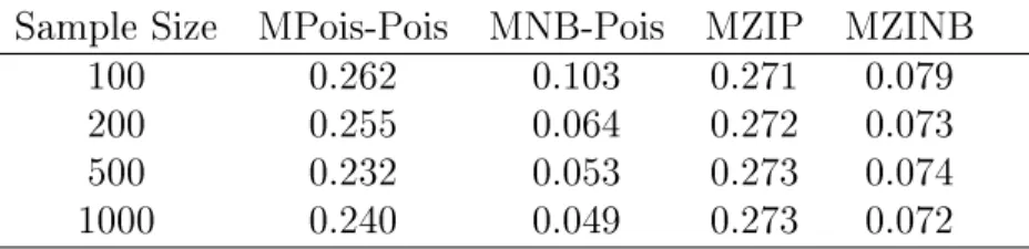
10,000 replications. . . 40 2.6 Type I error rates for the estimate ofβ1from
marginal-ized models tted to data generated from the
MNB-Pois model with 10,000 replications. . . 40 2.7 Coverages of 95% condence intervals for estimates
of β1, β2 and β3 from marginalized models tted
to data generated from the MNB-Pois model with
10,000 replications. . . 41 2.8 Percentages of converged marginalized models tted
to data generated from the MNB-Pois model with
10,000 replications. . . 41 2.9 Estimated log-likelihood, AIC and incidence density
ratios (95% CI) comparing NaF and NaFTMP with
SMFP in the Lanakshire trial, based on four
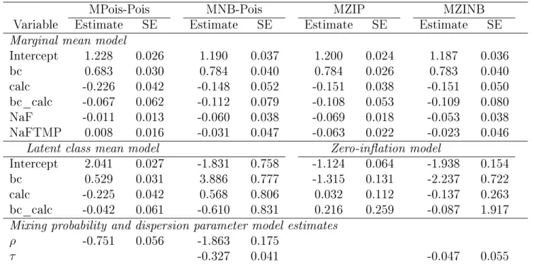
marginal-ized models. . . 44 2.10 Marginal mean model Estimates and standard
er-rors from MPois-Pois, MNB-Pois, MZIP and MZINB
3.1 Percent relative median biases and coverages of 95% condence intervals of MBZIP and MZIP model
es-timates based on 10,000 replications. . . 61 3.2 Percent relative median biases, mean standard
er-rors, Monte Carlo standard deviations and coverages of 95% condence intervals of nuisance parameters in the MBZIP models, based on data generated from
the MBZIP model with 10,000 replications. . . 62 3.3 Mean standard errors and Monte Carlo standard
de-viations of MBZIP and MZIP model estimates, based on data generated from the MBZIP model with 10,000
replications. . . 63 3.4 Type I errors of β11 andβ21 from MBZIP and MZIP
models based on Wald type tests, based on data
gen-erated from the MBZIP model with 10,000 replications. . . 64 3.5 Parameter estimates and standard errors for the NC
FMR data based on MBZIP and MZIP models. . . 65 3.6 Continued: parameter estimates and standard errors
for the NC FMR data based on MBZIP and MZIP models. . . 66 4.1 Simulation results for scenario with two covariates,
where one is potentially missing: comparison of MCEM and CC models based on 500 replications with
sam-ple sizes 250, 500 and 1000. . . 85 4.2 Simulation results for scenario with three covariates,
where two are potentially missing: comparison of MCEM and CC models based on 500 replications
with sample size 1000 for two missing data scenarios. . . 86 4.3 MZIP estimates and standard errors for the NC FMR
data from MCEM, multiple imputation and
LIST OF FIGURES
2.1 Distribution of DFMS counts after 2 years for 3412 children ages 11-12 participating in the Lanarkshire
trial. . . 42 2.2 Predicted and observed proportions of DMFS count
increments after 2 years in the Lanarkshire trial. . . 43 3.1 Distributions of dmfs and DFMS counts from 677
children in the NC FMR study. . . 60 4.1 Distribution of dmfs counts from 1094 children grades
1 to 5 participating in a school-based uoride mouthrinse
CHAPTER 1: LITERATURE REVIEW
1.1 Introduction
The analysis of counts generated from heterogeneous populations present special chal-lenges to researchers. When data arise from several unobserved subpopulations, models based on standard probability distributions are often inadequate to explain observed vari-abilities (Wedel and DeSarbo, 1995; Frühwirth-Schnatter, 2005). One example would be the case of zero-inated counts, where proportions of zero observations are higher than expected under standard distributions. Employing traditional distributions (such as the Poisson) to model such data often results in biased estimates and poor predictions (Lam-bert,1992). Instead, zero-inated counts are commonly modeled by using two-component mixture distributions, hypothesizing that observations arise from two latent classes within the source population: one class provides only zeros and the other produces both zero and non-zero values. Such an approach is under the framework of nite mixture modeling, which partitions a source population into a number of unobserved classes or subpopulations and estimates parameters specic to the latent classes. Common models for counts with excess zeros such as zero-inated Poisson (ZIP) regression utilize two-component mixtures consisting of a degenerate zero and a standard count distribution.
bivariate zero-inated counts.
Despite the exibility that mixture distributions provide in modeling highly dispersed count data, interpretations of the regression parameters from such models are limited to the latent classes making up the study population. These parameters are not directly applicable to making inferences about the overall eects of covariates on the marginal mean. Even with the application of indirect methods of parameter estimation such as the use of post-modeling transformations, there are many instances where latent class model formulations fail to fully explain relationships between covariates and population-wide parameters (Preisser et al.,2012; Long et al., 2014).
maximum likelihood estimation. In the second part, we propose a marginalized model for bivariate zero-inated counts that provides directly interpretable regression parameters for the marginal means of the two correlated outcomes in the overall population.
While much of the statistical literature on zero-inated data modeling treats covariates and outcomes as fully observed, missing data are a common occurrence in practice. In the absence of appropriate statistical software and methods to deal with incomplete data, modeling is typically done by using only cases with complete covariate and outcome data (Ibrahim et al., 2005). However, this approach, often referred to as complete case analysis, is valid only when the probability of missingness is independent of any observed and unob-served information. Even when complete case analysis is valid, estimates can be inecient if too many observations are missing (Ibrahim et al., 1999, 2005). For problems where co-variates are missing at random and their conditional distribution is log-concave, Ibrahim et al.(1999) propose a Monte Carlo EM (Wei and Tanner, 1990) algorithm to allow for max-imum likelihood estimation. Although the method can be adapted to ZIP regression with missing covariates, it is not directly applicable to marginalized zero-inated models because the corresponding conditional densities may not be written as products of log-concave dis-tributions. In the third part of the dissertation, we extend the Monte Carlo EM approach to marginalized zero-inated Poisson models with missing covariates
1.2 Mixture Models
Mixture distributions have been used to model observations with variabilities that are insuciently explained by standard statistical models. An underlying assumption of such models is that variability in observations is due mainly to heterogeneity within the sam-pled population, which may contain a number of unobserved subpopulations of unknown proportions (Wedel and DeSarbo, 1995). In discrete modeling, a simple but popular mix-ture is that of the Poisson and gamma distributions (i.e, the negative binomial), which is commonly used to model counts with extra-Poisson dispersion. The Poisson and nega-tive binomial distributions are also often mixed with a distribution degenerate at zero to model counts with much higher proportions of zeros than expected under either of these two standard distributions. These models presume that observations arise from a popu-lation containing two unobserved subpopupopu-lations; while one subpopupopu-lation produces only zero counts, observations from the other subpopulation can have zero or positive values. Because such assumptions lead to data generating mechanisms that conveniently explain heterogeneities in counts in various research problems, the two component mixture model has been given a lot of attention over the past few decades (Lambert, 1992; Mullahy, 1986; Heilbron, 1994; Bo¨hning et al., 1999). Mixtures involving more than two component
distri-butions have also been applied in the health sciences, medicine, genetics, economics, ecology and other areas (Wang et al., 1996, Morgan et al., 2014).
Finite mixture models partition a source population into m ≥ 2 latent subpopulations
and assume that the random variable of interest takes a value from the jth subpopulation with a probabilityπj. IfYi is count random variable with observed valueyi, anmcomponent mixture distribution can be dened for Yi as (Frühwirth-Schnatter, 2005)
P r(Yi =yi∣π,θi)= m ∑ j=1
πjfj(yi∣θij), (1.1)
θij is the vector of parameters infj,θi =(θi1,θi2, ...,θim), andπ=(π1, π2..., πm)′ is a vector
of mixing probabilities with 0≤πj ≤1 and ∑mj=1πj =1. The latent parameters πj and θij corresponding to the jth component are also estimated either as constants or as functions of covariates through convenient link functions. For example, if θij is a scalar and xi is a vector of covariates from theith subject, then θ
ij can be related to the covariates as
θij(βj)=g−1(x′iβj), (1.2)
where βj is a vector of regression parameters corresponding to the jth component and g is a link function. While the mixture model in equation (1.1) imposes heterogeneity only
through fj(yi∣θij), the mixing probabilities (i.e., πj) may also be allowed to vary across individuals.
1.2.1 Poisson and Negative Binomial Mixtures
Finite Poisson mixtures are one of the popular mixture models for count data. In these models, fj, j=1,2, ..., m in equation (1.1) has the form
fj(yi∣µij)=
e−µijµyi
ij yi!
, (1.3)
where µij is a mean parameter. While earlier applications of Poisson mixtures estimate model parametersπj andµij as constants, Wang et al.(1996) introduce covariates to model the latent class mean parameters as
log(µij)=x′iβj, j =1,2, ..., m, (1.4)
implement the expectation maximization (EM) algorithm together with quasi-Newton max-imization to perform estimation.
To account for extra-Poisson dispersion within each latent subpopulation, Ramaswamy, Anderson and DeSarbo (1994) propose negative binomial mixture models, for which the component distributions in equation (1.1) are negative binomial. That is,
fj(yi∣θij)=
Γ(yi+αj) yi!Γ(αj)
( αj αj+µij
)αj( µij αj+µij
)yi, (1.5)
where µij is the mean parameter, αj is the dispersion parameter and θij =(µij, αj). Ra-maswamy, Anderson and DeSarbo (1994) model the mean parameters as functions of co-variates and estimate the mixing probabilities and dispersion parameters as constants using the EM algorithm.
1.3 Analysis of Zero-inated Counts
Oftentimes, counts collected in various research areas contain high proportions of zeros. One such area is dental caries research, where counts of decayed, missing and lled teeth (dmfs) are increasingly characterized by disproportionately high numbers of zeros (Lewsey and Thompson, 2004; Mwalili et al., 2008; Preisser et al., 2012; Albert et al., 2014). Be-cause of the excess number of zero observations relative to what is expected under standard probability distributions, traditional generalized linear models do not suciently explain variability in such counts. For instance, while the Poisson distribution assumes equality of means and variances, the variances of zero-inated counts are generally larger than the corresponding means. As a result, Poisson regression models tend to underestimate propor-tions of zeros and those of large positives when tted to counts with excess zeros (Lambert, 1992).
of these models assume that counts originate from two latent subpopulations, and can in general be divided into two categories depending on how they treat the generation of zero and positive counts from the two latent groups. The rst category of models, often called zero-inated models (Long et al., 2014), presume that both zero and positive counts arise from one latent subpopulation according to a standard probability distribution, but extra zeros come from a second latent subpopulation based a distribution degenerate at zero. Zero-inated Poisson (ZIP) regression is one of such models, and has been increasingly popular after Lambert (1992) described the data generating processes and applied it to defects in manufacturing processes. When zero-inated counts show variabilities that are not attributed to excess zeros, the Poisson distribution in ZIP is often replaced by a negative binomial probability function, resulting in the zero-inated negative binomial (ZINB) model. Hurdle or zero-altered models (Mullahy, 1986) comprise of the second category of estimation methods for zero-inated data, where zero and positive counts are considered to come from two separate latent subpopulations. In hurdle models, regression parameters are often specied for the logit of the probability of a count being positive and the mean of the untruncated version of the distribution assumed for positive counts.
1.3.1 ZIP and ZINB Regression Models
assumes that the random variable Yi, i=1,2, ..., n, takes zero or positive values as follows (Long et al., 2014).
Yi∼⎧⎪⎪⎪⎪⎨ ⎪⎪⎪⎪ ⎩
0, with probabilityψi Poisson(µi), with probability1−ψi
(1.6)
In (1.6), ψi is the probability of being from the `perfect' or `non-susciptible' subpopu-lation, and µi is the mean of the Poisson distribution corresponding to the `imperfect' or `susceptible' group. Considering ψi as a mixing probability, the distribution of Yi can be written in the form of equation (1.1) as
P r(Yi =k)=ψiI(k=0)+(1−ψi)g(k∣µi), k=0,1,2, ..., (1.7)
where g is the Poisson mass function and I(T) is an indicator variable taking the value 1
when T is true and the value 0 when T is false. Clearly, when the mixing parameter ψi is zero, ZIP reduces to the standard Poisson model. By using the logit and the log links, Lambert (1992) allows the probability of membership in the `perfect' state, ψi, and the Poisson mean, µi, to depend on covariates as
logit(ψi)=z′iγ and log(µi)=x′iβ (1.8)
In (1.8), zi and xi are q×1 and p×1 vectors of covariates for the ith subject, and γ = (γ1, γ2, . . . , γq)and β=(β1, β2, . . . , βp)are regression parameters. Usually, the set of
covari-ates in zi is a subset of those inxi.
The variance and the marginal mean of a ZIP random variable Yi are, V ar(Yi∣zi,xi)=
µi(1−ψi)+µ2
For problems where ψi and µi are believed to be related, Lambert (1992) species shared regression coecients to model the two latent parameters.
log(µi)=x′iβ and logit(ψi)=τx′iβ, (1.9)
where τ is a parameter to be estimated. Note that the specication in (1.9) reduces the
number of regression parameters by almost half.
To estimate the parameters β andγ in equation (1.8), Lambert (1992) employs the EM
algorithm on a complete data log-likelihood function involving a binary latent variable that denes membership in either of the two latent subpopulations. For the shared parameter ZIP model in equation (1.9), estimation is performed using Newton-Raphson algorithm.
Zero-inated negative binomial models are similarly formulated as ZIP by using a neg-ative binomial probability mass function g in (1.7). In addition to zero-ination, ZINB
models allow for the handling of overdispersion caused by unobserved heterogeneities.
1.4 Models for Bivariate Zero-inated Counts
propose mixtures comprising a multivariate distribution degenerate at zero values, a mul-tivariate Poisson distribution and a number of univariate Poisson distributions. For the bivariate case, they assume that a zero-inated random variable(Y1, Y2) arises either from
a distribution degenerate at(0,0), from a bivariate Poisson distribution, or from a bivariate
distribution with one component degenerate at 0 and the other having a standard Poisson mass function. That is,
(Y1, Y2)∼
⎧⎪⎪⎪ ⎪⎪⎪⎪⎪ ⎪⎪⎪⎪ ⎨⎪⎪ ⎪⎪⎪⎪⎪ ⎪⎪⎪⎪⎪ ⎩
(0,0),with probabilityp0
(Poisson(λ1),0),with probabilityp1
(0,Poisson(λ2)),with probabilityp2
Bivariate Poisson(λ10, λ20, λ00), with probabilityp3,
(1.10)
where pk ≥ 0, k = 0,1,2,3, ∑3k=0pk = 1, and λ1, λ2, λ10, λ20, λ00 > 0. The bivariate
distribution in (1.10) reduces to the standard bivariate Poisson model for p0 =p1 =p2 =0.
When λ1 =λ10+λ00 and λ2 =λ20+λ00 in equation (1.10), the marginal distributions of Y1
and Y2 become univariate ZIP. That is,
Pr(Yt=k)= ⎧⎪⎪⎪ ⎪⎨ ⎪⎪⎪⎪ ⎩
(1−pt−p3)+(pt+p3)exp(−λt), k=0
(pt+p3)
exp(−λt)λk t
k! , k=1,2, ...
(1.11)
wheret=1,2. Li et al.(1999) employ directional grid search approaches (Powell, 1964) and
methods of moments to obtain maximum likelihood estimates of model parameters.
When covariates are used to model bivariate zero-inated Poisson counts, linear predic-tors are specied for the mean parameters and the mixing probabilities, for example, as
log(λ10i) = x′1iα1, log(λ20i) = x′2iα2, log(λ00i) = x′3iα3, log(p0i/p3i) = x′4iγ0, log(p1i/p3i) = x′5iγ1 and log(p2i/p3i)=x′6iγ2, wherex1i, ..., x6i are vectors of covariates from the ith indi-vidual, and α1,α2, α3,γ0, γ1 and γ2 are vectors of parameters (Li et al., 1999; Majundar
to employ post-modeling transformations to estimate the eects of covariates on the over-all population means ν1i = E(Y1i) and ν2i = E(Y2i). The marginal means and the model
parameters can be related by
ν1i=(p1i+p3i)(λ00i+λ10i)=
(ex′1iα1 +ex′3iα3)(1+ex′5iγ1)
1+ex′4iγ0+ex5′iγ1+ex′6iγ2 (1.12)
ν2i=(p2i+p3i)(λ00i+λ20i)= (
ex′2iα2 +ex′3iα3)(1+ex′6iγ2) 1+ex′4iγ0+ex′5iγ1+ex′6iγ2
Althoughν1i and ν2i could be estimated at xed covariate values by using equations (1.12), the quantication of the relationship between covariates and the marginal means with suit-able variance estimates may be dicult in practice. In addition, when interest is in deter-mining whether the eects of an exposure on ν1i or ν2i are homogeneous across the levels of covariates, existing bivariate zero-inated models usually do not provide the desired es-timates as in the case of traditional zero-inated models for univariate counts (Long et al., 2014).
1.5 Inference About the Overall Population
density ratios, it has been indicated that ZIP and ZINB models may not always provide the desired estimates (Long et al., 2014). For example, consider a clinical trial where the ZIP regression in equation (1.8) is used to model a zero-inated outcome variable with zi = xi. From the relationνi=µi(1−ψi), whereνi=E(Yi∣xi), the overall mean for theith subject is
νi= e
x′iβ
1+ex′iγ (1.13)
The incidence density ratio (IDRi) or the ratio of overall means corresponding to a one unit increase in the jth exposure variable, x
ij, is (Long et al., 2014),
IDRi=
E(yi∣xij =c+1,x˜′i =x˜′i) E(yi∣xij =c,x˜′i =x˜′i)
=eβj 1+exp(cγj+x˜
′
iγ˜)
1+exp((c+1)γj+x˜′iγ˜)
, (1.14)
where x˜i is the vector of covariates without xij, c is a possible value of xij and γ˜ is the vector of parameters in the logit model corresponding to x˜i (Preisser et al., 2012; Long et al., 2014). When γj ≠0 in equation (1.14), the estimate of IDRi changes as the values of the covariates in x˜i change. In other words, ZIP regression parameters do not allow the estimation of an overall constant incident density ratio when the exposure variable of interest is included in the logit model (Long et al., 2014).
In the literature, several approaches have been proposed for the estimation of overall eects of explanatory variables on population-level parameters. While many of these meth-ods involve tting traditional zero-inated models and then using the estimates to describe the parameters of interest, more recent approaches specify regression coecients directly for the marginal mean.
1.5.1 Estimation Based on Latent Coecients
defect counts as levels of manufacturing settings change, Lambert (1992) estimates the over-all population mean at a level of a categorical covariate by averaging the model estimated means across all design points sharing the specic level of the covariate. This way, compar-isons are made among levels of a covariate with regard to the overall mean of manufacturing defects. Although the method can be employed for problems where all involved predictor variables are categorical, it may not be appropriate when the ZIP model includes one or more continuous covariates. In a further attempt to characterize the overall population mean, Böhning et al.(1999) propose large sample methods to construct (1−α)100%
con-dence intervals for the marginal mean, ν, as Y¯ ±z(1−α
2)
√ V ar(Y)
n , where Y¯ is the observed mean count,V ar(Y)is the variance, n is the sample size andz(1−α2) is the1−α2 quantile of
the standard normal distribution.
1.5.2 Marginalized Models
To estimate directly interpretable regression parameters for marginal means of ZIP dis-tributed counts, Long et al.(2014) propose marginalized zero-inated Poisson (MZIP) mod-els, where regression parameters are specied for the overall population mean as well as for the probability of being an excess zero. Preisser et al.(2016) extend MZIP models to handle counts with extra-Poisson dispersion in addition to zero-ination, by using the ZINB likelihood function. As in MZIP, the marginalized zero-inated negative binomial (MZINB) regression provides coecients for the eects of covariates on the marginal means as well as for the excess zero probabilities.
LetYi be a random variable having a ZIP distribution with marginal meanνi and excess zero probabilityψi. The MZIP model relatesνi andψi with covariates as (Long et al., 2014)
logit(ψi)=z′iγ (1.15)
log(νi)=x′iα,
In (1.15), zi and xi are q×1 and p×1 vectors of covariates, and the parameters in γ = (γ1, γ2, ..., γq)′ have the same interpretation as in standard ZIP models. Unlike ZIP models,
however, parameters α = (α1, α2, ..., αp)′ describe heterogeneity in the overall population mean, instead of the mean count for subjects in the `susceptible' latent class. Since the mean µi of the Poisson part of ZIP and the overall mean νi are related byνi=(1−ψi)µi=ex
′
iα, to
nd the MZIP likelihood, Long et al.(2014) replaceµiby 1−νiψi in the ZIP likelihood function. Thus, forn independent subjects, the log-likelihood function for MZIP models is written as
ℓ(γ,α∣y) = −
n ∑ i=1
log(1+ez′iγ)+
n ∑ i=1
I(yi =0)log{ez
′
iγ +e−(1+exp(z′iγ))exp(x′iα)}
+ ∑n i=1
I(yi>0){−(1+ez
′
iγ)ex′iα+y
ilog(1+ez
′
iγ)+y
The corresponding score equations are (Long et al., 2014),
∂l(α,γ)
∂γ =
n ∑ i=1
[I(yi=0)ψi(1−ψi)−1(eνi(1−ψi)
−1 −νi) ψi(1−ψi)−1eνi(1−ψi)−1
+1 (1.16)
+ ψi(yi−1)−I(yi>0)ψi(1−ψi)−1νi]z′i ∂l(α,γ)
∂α = −
n ∑ i=1
[ I(yi=0)νi(1−ψi)−1 ψi(1−ψi)−1eνi(1−ψi)−1
+1−(yi−νi(1−ψi) −1)I(y
i>0)]x′i
Long et al.(2014) employ quasi-Newton optimization methods to obtain parameter esti-mates. The variance covariance matrix of the parameters is obtained by inverting the expected information matrix. For the case in which the counts are over-dispersed relative to ZIP, robust standard errors are estimated.
For MZINB models, in addition to the standard regression parameter specications for ψi and νi as in (1.15), Preisser et al (2016) model ψi by using shared parameters from the linear predictor of νi as
logit(ψi)=γ0+γ1(x′iα) (1.17) log(νi)=x′iα,
where γ0 and γ1 are scalar parameters.
1.6 Missing Data
adjustments, and variable deletion (Allison, 2002). The use of such methods, however, may result in biased estimates, reduced eciency and model mis-specications (Allison, 2002).
Over the past few decades, much attention has been given to missing data methods for a wide range of models. In general, such methods work under certain assumptions about the dependence of the missingness mechanism on observed and missing values of relevant variables. Based on the nature of missingness, Little and Rubin (2002) group missing data into three categories: missing completely at random (MCAR), missing at random (MAR) and not missing at random (NMAR). Under MCAR, missingness is independent of any observed or unobserved information, and the MAR assumption holds when missingness is independent of any unobserved data. NMAR has the weakest assumptions among the three categories, and assumes that the probability of missingness is dependent on missing data. In maximum likelihood estimation, when data are MAR and the model of interest and missingness mechanism have separate parameters, missingness is ignorable, meaning that estimation can be done without modeling the missing data mechanism (Ibrahim et al., 2005). However, NMAR data require specication of a model for the missingness mecha-nism as part of the estimation process (Ibrahim et al., 1999, 2005). Maximum likelihood methods for missing data often estimate model parameters either by directly maximizing the observed data likelihood or by using the expectation-maximization algorithm on a con-venient complete data likelihood function (Allison, 2002). However, since computing and maximizing the observed data likelihoods is often dicult, many of maximum likelihood based missing data methods rely on the EM algorithm and related approaches.
1.6.1 EM Algorithm and Monte Carlo EM Methods
convergence is attained. While the expectation or E-step of EM computes the expected value of the complete data log-likelihood conditional on the observed data and current parameter values, the maximization or M-step maximizes the expected log-likelihood. In situations where the E-step is dicult to compute, the Monte Carlo EM (MCEM) algorithm (Wei and Tanner, 1990) may be employed to estimate the log-likelihood numerically. Ibrahim et al.(1999) apply the method for missing covariates in parametric models by using samples obtained from the Gibbs sampler with adaptive rejection sampling (ARS) algorithm (Gilks and Wild, 1992). Following Ibrahim et al.(1999, 2005), we review the applications of EM and MCEM methods for missing covariate problems in count models. In the following discussions, the outcome variable is assumed to be fully observed, but covariates can have missing values for some of the the study subjects.
Suppose that y = (y1, y2, . . . , yn)′ is a vector of independent count outcomes from n
subjects. For the ith subject, let x
i = (xi1, xi2, . . . , xip)′ be a p×1 vector of covariates.
Because covariates are partially missing for some subjects, Ibrahim et al.(1999, 2005) write the covariate vectorxi asxi =(xobsi ,xmisi ), withxobsi andxmisi representing the observed and the missing parts ofxi, respectively. Using these notations, the observed data vector for the
ith subject is (y
i,xobsi ,ri), where ri = (ri1, ri2, . . . , rip) is a vector of missingness indicators
for components ofxi, dened by,
rij = ⎧⎪⎪⎪ ⎪⎨ ⎪⎪⎪⎪ ⎩
1, if thejthcomponent of x
i is observed.
0, otherwise.
(1.18)
Under MAR, the conditional distribution of ri given the data is a function only of the observed information and is independent of the missing data. Thus,
joint distribution of (yi,xi),missingness is ignorable and estimation can be done based on the likelihoodLfrom the outcome and the covariates, whereLis often written as a product of the conditional distribution of the outcome given the covariates and the joint distribution of the covariates as (Ibrahim et al., 1999)
L(ξ,α,γ∣y,xobs,xmis)=
n ∏
i=1
P r(yi∣xobsi ,xmisi ,α,γ)P r(xmisi ∣xobsi ,ξ) (1.20) =∏n
i=1
Li(ξ,α,γ∣yi,xobsi ,xmisi ),
where α and γ are parameter of the model that are of primary interest, ξ is a vector of parameters in the joint distribution of the missing covariates. Note that the conditional distributionsP r(xmis
i ∣xobsi ,ξ)are used in (1.20) since the joint distribution of the covariates is proportional to the distribution of the missing covariates conditional on the observed (Ibrahim et al., 1999, 2005). From (1.20), the complete data log-likelihoodℓ(θ∣y,xobs,xmis) can be written as
ℓ(θ∣y,xobs,xmis)=
n ∑ i=1
ℓ(η∣yi;xobsi ,xmisi )+ n ∑ i=1
ℓ(ξ∣xmisi ;xobsi ) (1.21)
=∑n i=1
ℓi(θ∣yi,xobsi ,xmisi )
whereθ=(α,γ ,ξ),η=(α,γ),ℓ(η∣yi;xobsi ,xmisi )=log(P r(yi∣xobsi ,xmisi ,η)) andℓ(ξ∣xmisi ;
xobs
i )=log(P r(xmisi ∣xobsi ,ξ)).
t is θ(t), at the (t+1)th iteration, the E step of EM computes,
Qi(θ∣θ(t))=E(ℓc(θ∣yi,xobsi ,xmisi )∣yi,xobsi ,θ(t)). (1.22)
In (1.22),ℓcis the log-likelihood from the complete data. The M-step of EM then maximizes Q(θ∣θ(t)) = ∑n
i=1Qi(θ∣θ(t)) to obtain the parameter estimates at iteration t+1, and the
process continues until convergence. Values of θ obtained at convergence are maximum likelihood estimates and the corresponding covariance matrix is commonly obtained using the method of Louise (1982).
For problems where a direct evaluation of the E-step is dicult, Monte Carlo EM meth-ods estimate the expected log-likelihood numerically. At iterationt+1, the MCEM approach
generates Monte-Carlo samples of size, says, from the conditional distribution of the missing covariates and estimatesQi(θ∣θ(t)) in equation (1.22) by (Ibrahim et al., 1999),
Qi(θ∣θ(t))= 1 s
s ∑ j=1
ℓ(θ∣yi,dij,xobsi ) (1.23)
where di1,di2, . . .and,dis are vectors of Monte-Carlo samples from the conditional distri-butions of the missing covariates. Ibrahim et al.(1999) generate Monte Carlo samples using adaptive rejection algorithm with Gibbs sampling for problems where the conditional dis-tributions P r(yi∣xobs
CHAPTER 2: MARGINALIZED MIXTURE MODELS FOR COUNT DATA FROM MULTIPLE SOURCE POPULATIONS
2.1 Introduction
post-modeling transformations, there are many instances where latent class model formula-tions fail to fully explain relaformula-tionships between covariates and population-wide parameters. While the importance of the marginal mean as a target of inference in the analysis of nite mixtures of counts is well established (Lambert, 1992; Bo¨hning et al., 1999; Preisser
et al., 2012; Albert et al., 2014), marginally-specied mean models for nite mixtures of count distributions have more recently been proposed. Within a ZIP likelihood framework, Long et al.(2014) proposed marginalized zero-inated Poisson (MZIP) regression, which species a two-part model for counts with a set of regression coecients for the marginal mean and, to complete model specication, a second set of regression coecients for the latent parameter dening membership in the `excess-zero' class. The marginalized zero-inated negative binomial (MZINB) model (Preisser et al., 2016) extended the MZIP model to zero-inated negative binomial (ZINB) distributions. Todem et al.(2016) described a general representation of two-part marginalized mean count models including distributions for bounded counts, e.g., the zero-inated beta binomial distribution. All these marginalized models assume that the count outcomes follow two-component mixtures consisting of a standard count distribution with a point-mass at zero. Data-generating mechanisms based on mixtures of non-degenerate count distributions could provide better ts in the class of marginalized mixture models for count data.
the combination of sodium uoride and sodium trimetaphosphate (Stephen et al., 1994; Preisser et al., 2013). The outcome variable of interest was the number of new decayed, missing and lled surfaces (DMFS) and dental exams were performed at baseline and after 1, 2 and 3 years. Because the DMFS counts exhibit many zeros, Poisson or negative binomial regression is not appropriate to model the counts. We consider marginalized, two-component nite mixture models to obtain direct inference about the relationship between toothpaste formulation and the marginal mean caries count in the trial population. Section 2.2 reviews zero-inated mixture distributions and marginalized zero-inated models, while Section 2.3 briey discusses traditional nite mixture models. Section 2.4 presents two dierent two-component marginalized mixture models involving non-degenerate distributions. Simulation studies and an application of the proposed models are discussed in Sections 2.5 & 2.6 respectively. Concluding remarks follow in Section 2.7.
2.2 Models for Zero-inated Data
2.2.1 Zero-inated Poisson and Negative Binomial Models
zero-inated Poisson or negative binomial distribution can be written as
P r(Yi =k)=πiI(k=0)+(1−πi)g(k∣θi), k=0,1,2, ..., (2.24)
where the mixing parameter πi is interpreted as the probability of a count being from the `non-susceptible' or `not-at-risk' latent class,I(T)is an indicator variable taking 1when T is true, and 0 when T is false; g is a Poisson or negative binomial mass function, and θi is the vector of parameters in g. Wheng is the Poisson mass function,θi is equal to the mean µi of the distribution, and for a negative binomial probability mass functiong, θi=(µi, α), where µi is the mean of the distribution and ϕ is the dispersion parameter. In this paper we will use the following parameterization for the probability mass function of a negative binomial distribution with mean µand dispersion parameter α.
f(y∣µ, α)= Γ(y+α) y!Γ(α) (
α α+µ)
α ( µ
α+µ) y
, where y=0,1, . . . . (2.25)
In zero-inated models, regression parameters are specied for the mixing probabilityπi and the mean of the assumed standard distributionµi, by using the logit and the log links as in equation (3) of Preisser et al.(2016), as
logit(πi)=z′iγ and log(µi)=x′iξ, (2.26)
where zi and xi are q×1 and p×1 vectors of covariates for the ith subject, and γ = (γ1, γ2, . . . , γq)′ and ξ=(ξ1, ξ2, . . . , ξp)′ are regression parameters.
For n independent observations, the ZIP likelihood function is
L(ξ,γ∣y)=
n ∏ i=1
{1+e(z′iγ)}−1{e(z′iγ)+e−exp(x′iξ)}I(yi=0){e
−exp(x′iξ)ex′iξyi
yi!
} I(yi>0)
The corresponding likelihood function for the ZINB model can be written as
L(ξ,γ∣y) =
n ∏
i=1
{1+e(z′iγ)}−1{e(z′iγ)+( α
α+ex′iξ)) α
}I(yi=0) (2.28)
× ∏n i=1
{Γ(yi+α) yi!Γ(α)
( α
α+ex′iξ)) α
( ex
′
iξ
α+ex′iξ)) yi
} I(yi>0)
Since interpretations of parameters γ and ξ in ZIP and ZINB models apply to the two latent subpopulations, they do not directly describe the overall population mean. Although the overall mean, E(Yi)=νi, forith subject could be estimated from such models by
νi = ex′iξ
1+ez′iγ (2.29)
and transformations such as the delta method could be applied to estimate the correspond-ing variance, it is not always easy to understand the behavior ofνi. In particular, determin-ing the eects of an exposure variable on incidence density ratios is challengdetermin-ing especially when the linear predictor for the mixing proportions contain some of the covariates in the Poisson mean model (Long et al., 2014).
2.2.2 Marginalized ZIP and ZINB Models
To estimate the overall eects of covariates on the population mean, marginalized zero-inated Poisson (Long et al., 2014) and marginalized zero-inated negative binomial (Preisser et al., 2016) models specify parameters for the marginal meanνi=E(yi)=(1−πi)µi and the probability of being an excess zero (i.e., πi) as
log(vi)=x′iβ and logit(πi)=z′iγ, (2.30)
where β=(β1, β2, ..., βp) is a vector of regression parameters for νi, and the parameters in
likelihood functions are obtained by replacing µi by 1−νiπi in the ZIP and ZINB likelihoods, respectively.
2.3 Finite Mixture Models
Finite mixture distributions have been used to model counts obtained from heteroge-neous populations (Wang et al., 1996; Morgan et al., 2014; Schlattmann et al., 2009). In the nite mixture model, the source population is assumed to be a partition of latent sub-populations; with a probability πij, the count random variable Yi corresponding to the ith individual takes a value from the jth subpopulation according to a distribution specic to the subpopulation. An m component mixture distribution can be dened as (Wedel and DeSarbo, 1995; Frühwirth-Schnatter, 2005)
P r(Yi =yi∣π,θij)= m ∑ j=1
πjfj(yi∣θij), (2.31)
where the components f1,f2, ..., fm are probability mass functions of known distributions, θij is the vector of parameters in fj, and π = (π1, π2..., πm)′ is a vector of mixing
proba-bilities with 0 ≤ πj ≤ 1 and ∑mj=1πj = 1. While the mixture distribution for zero-inated counts in equation (2.24) allows mixing probabilities (i.e., πi) to vary across individuals,
conventional nite mixture models assume a constant probability, πj, corresponding to the jth subpopulation and impose heterogeneity throughf
j(yi∣θij). The Poisson mixture distribution, where
fj(yi∣µij)=
e−µijµyi
ij yi!
for full rank design matrices. While nite mixture models enable exible modeling of counts from heterogeneous populations, their parameters have latent class interpretations. Such coecients do not enable one to make direct inferences of the eects of covariates on the overall population mean (Roeder et al., 1999; Min and Agresti, 2005).
2.4 Marginalized Finite Mixture Models
In this section we propose methods of estimating regression parameters for the overall population mean of zero-inated and other types of heterogeneous counts by employing non-degenerate mixture distributions. With the aim of expanding the pool of marginalized models for such counts, we consider data generating mechanisms based on mixtures of two Poissons (Pois-Pois) and a negative binomial and a Poisson (NB-Pois) distributions.
2.4.1 Models
The probability mass function (pmf) of a random variable with a Pois-Pois mixture distribution can be written as
f(yi∣π, µ1i, µ2i)=πfP1(yi∣µ1i)+(1−π)fP2(yi∣µ2i), (2.32)
where π is a mixing probability,and fP1 and fP2 are Poisson mass functions with
corre-sponding mean parameters µ1i and µ2i. Similarly, a NP-Pois random variable has a pmf
given by,
f(yi∣πi, µ1i, µ2i, α)=πfP(yi∣µ1i)+(1−π)fN B(yi∣µ2i, α). (2.33) In (2.33), fP is a Poisson pmf with mean parameter µ1i and fN B a negative binomial pmf with mean and dispersion parameters µ2i and α, respectively. The marginal mean, νi, of a random variable Yi having either of the two mixture distributions can be written as
Solving for µ2i in equation (2.34) gives
µ2i =
νi−πµ1i
1−π . (2.35)
To estimate a model for νi, the likelihood functions of Pois-Pois and NB-Pois mixture models can be written as functions of νi using equation (2.35) and replacing µ2i by a linear function of the marginal mean. Thus, marginalized Poisson-Poisson (MPois-Pois) and marginalized NB-Poisson (MNB-Pois) models dened immediately below can be estimated utilizing the pmfs in equations (2.36) and (2.37), respectively.
fM P P(yi∣π, µ1i, νi)=π
e−µ1iµyi
1i
yi! +(1−π)
e−νi−1−πµπ1i[νi−πµ1i
1−π ] yi
yi! (2.36)
fN BP(yi∣π, α, µ1i, νi)=π
e−µ1iµyi
1i yi!
(2.37)
+(1−π)Γ(yi+α) yi!Γ(α)
( α
α+νi−πµ1i
1−π )α(
νi−πµ1i
1−π α+νi−πµ1i
1−π )yi
The MPois-Pois model is dened through the specication of generalized linear models for the relationship of covariates to νi and µ1i. Given a p×n design matrix X, a model for νi is specied as
log(νi)=x′iβ, (2.38)
parameterπ is modeled as a constant using the logit link. Thus, the complete marginalized Pois-Pois (MPois-Pois) model can be written as in equation (2.39).
log(νi)=x′iβ (2.39)
log(µ1i)=z′iξ
logit(π)=ρ,
wherexi andzi are vectors of covariates,β and ξ are vectors of regression coecients, and
−∞<ρ<∞is a constant.
Marginalized NB-Pois models require estimation of the dispersion parameter (i.e., α) in addition to the regression coecients in equation (2.39). We specify a model for α as
log(α)=−τ. (2.40)
The link functions in equations (2.39) and (2.40) correspond to νi >0, µ1i > 0, 0 <π <1 and α > 0. For n independent count random variables Y1, Y2, ..., Yn with corresponding
realizations y1, y2, ..., yn, the likelihood function for MPois-Pois models is given by (2.41).
L(ρ,β,ξ∣y)=
n ∏ i=0
1
(1+eρ)y i!
{eρexp(−ez′iξ)ez′iξyi+e−η(ρ,β,ξ;xi,zi)η(ρ,β,ξ;x
i,zi)yi}, (2.41)
with
η(ρ,β,ξ;xi,zi)=ex
′
iβ(1+eρ)−eρez′iξ. (2.42)
L(ρ, τ,β,ξ∣y)=
n ∏
i=0
Γ(yi+e−τ) (1+eρ)Γ(y
i+1)Γ(e−τ)
( e−τ
e−τ +η(ρ,β,ξ;x i,zi)
) e−τ
(2.43)
×∏n i=0
( η(ρ,β,ξ;xi,zi) e−τ+η(ρ,β,ξ;x
i,zi) )
yi
+∏n i=0
eρexp(−ezi′ξ)ez′iξyi
(1+eρ)y i!
,
where η(ρ,β,ξ;xi,zi)has the same interpretation as in equation (2.42).
2.4.2 Estimation
With carefully chosen starting parameter values, regression coecients in MPois-Pois and MNB-Pois models can be estimated by the use of quasi-Newton optimization. While MZIP or MZINB (Long et al., 2014; Preisser et al.,2016) model estimates can be used as starting values of coecients in the marginal mean model (i.e., the βs), starting values for coecients in the latent parameter models (i.e.,π, µi, and α) may be obtained from two-component Poisson-Poisson and negative binomial-Poisson models. Following Ramaswamy et al.(1994) and Leisch (2004), we employ EM algorithm to nd starting values for param-eters ρ, ξ and τ in MNB-Pois models. The same approach can be applied for MPois-Pois models.
2.4.3 Algorithm for Finding Starting Values of Parameters
for parameters π, µ1i, µ2i and α as
log(µ1i)=z′iγ (2.44)
log(µ2i)=x′iζ
π=π log(α)=−τ,
whereζ is a vector of parameters and all the other parameters and variables are as described in equations (2.39) and (2.40). In line with standard mixture models (Ramaswamy et al.,
1994; and Leisch, 2004), the logit link is not used to model π in equation (2.44); once π is estimated, a starting value for ρ in the marginal mean model can be obtained by setting ρ=logit(π).
As a complete data likelihood function is needed to implement EM algorithm, we dene an indicator variable Ui corresponding to the ith subject as (Ramaswamy et al., 1994; and Leisch, 2004)
Ui= ⎧⎪⎪⎪ ⎪⎨ ⎪⎪⎪⎪ ⎩
1, if subject i belongs to subpopulation 1
0, if subject i belongs to subpopulation 2
(2.45)
Thus, Ui has a Bernoulli distribution with parameter π.
P r(Ui =ui∣π)=πui(1−π)1−ui, ui =0,1.
The random variable (Yi, Ui) contains an observed outcome Yi and a missing variable Ui, and the contribution of (Yi, Ui) to the complete data likelihood is given by,
Lic(π,γ,ζ, τ∣ui, yi,xi,zi)=P r(Yi =yi∣γ,ζ, τ,xi,zi;Ui=ui)P r(Ui =ui∣π) (2.46) =[πfP(yi∣γ,zi)]
ui
The likelihood function Lc from n independent counts is the product of each likelihood in equation (2.46). That is (Ramaswamy et al., 1994),
Lc(π,γ,ζ, τ∣u,y,x,z)=
n ∏
i=0
[πfP(yi∣γ,zi)] ui
[(1−π)fN B(yi∣ζ, τ,xi)] 1−ui
. (2.47)
The log-likelihood function is given by
ℓc(π,γ,ζ, τ∣u,y,x,z)=
n ∑ i=0
[uilogit(π)+log(1−π)]+ n ∑ i=0
uilog(fP(yi∣γ,zi)) (2.48)
+∑n i=0
[(1−ui)log(fN B(yi∣ζ, τ,xi))]
Given initial parameter values θ(0)=(π(0),γ(0),ζ(0), τ(0)), the E step of EM computes the
expected value ofℓc conditional on the observed variables andθ(0).
E(ℓc(π,γ,ζ, τ∣u,y,x,z)∣θ(0),y,x,z))=
n ∑ i=0
[E(ui∣θ(0), yi,xi,zi)logit(π)+log(1−π)]
+∑n i=0
E(ui∣θ(0), yi,xi,zi)log(fP(yi∣γ,zi))
+∑n i=0
[log(fN B(yi∣ζ, τ,xi))(1−E(ui∣θ(0), yi,xi,zi))] (2.49) It can be shown that (Ramaswamy et al., 1994)
E(ui∣θ(0), yi,x,z)= π
(0)fP(yi∣γ,zi)
π(0)f
P(yi∣γ,zi)+(1−π(0))fN B(yi∣ζ, τ,xi)
Thus, the M step maximizes,
E(ℓc(π,β,ζ, τ∣u,y,x,z)∣θ(0),y,x,z))=
n ∑ i=0
[Pi(0)logit(π)+log(1−π)] (2.51)
+∑n i=0
Pi(0)log(fP(yi∣γ,zi))
+∑n i=0
[log(fN B(yi∣ζ, τ,xi))(1−P(
0)
i )]
=ℓπ+ℓγ+ℓ(ζ,τ)
To obtain the next estimates in the M step, the three componentsℓπ,ℓγ andℓ(ζ,τ) of the expected log-likelihood in (2.51), can be optimized separately. Maximizing ℓπ with respect toπ gives (Ramaswamy et al., 1994)
π(1)=
n ∑ i=0
Pi(0) n .
The remaining two components of the expected log-likelihood (i.e., ℓγ and ℓ(ζ,τ)) cor-respond to weighted log-likelihoods of generalized linear models and estimation can be performed separately to obtain the next set of parameters γ(1), ζ(1) and τ(1). Utilizing
the parameters (π(1),β(1),ζ(1), τ(1)) estimated in the rst step, EM again computes and
optimizes the expected log-likelihood and continues iterations between the two steps until convergence. The NB-Poisson mixture model estimates of π,γ and τ at convergence are then employed as starting values for parameters ρ =logit(π), ξ and τ respectively, in the MNB-Pois model.
2.5 Simulation Study
where π, µ1i, νi and α are determined from
log(νi)=x′iβ=β0+β1x1i+β2x2i+β3x3i (2.52) log(µ1i)=z′iξ=ξ0+ξ1x1i+ξ2x2i+ξ3x3i
logit(π)=ρ, log(α)=−τ
with xi =zi and x1i ∼ Poisson(2)/3, x2i ∼exp(1), x3i ∼Benoulli(0.4), β0 = 1.5, β1 =−0.1,
β2 = −0.2, β3 = 0.5, ξ0 = 1.5, ξ1 = −0.5, ξ2 = −0.5 , ξ3 = 1, ρ = −0.4 and τ = −0.5. Using
these specications, samples of sizes 100, 200, 500 and 1000 were generated correspond-ing to marginalized Pois-Pois and NB-Pois models. Four marginalized models, namely, MPois-Pois, MNB-Pois, MZIP and MZINB models were then tted to the data, where each simulation was repeated 10,000 times. To estimate Type I error rates of testing H0 ∶ β1 = 0 vs H1 ∶ β1 ≠0, all the simulations were repeated by generating data using
β1=0, but keeping all the remaining parameter and covariate values the same as described
previously. For each of the four models, the Type I error rates were calculated as the pro-portion of 10,000 models that converged and estimated a p-value from two-sided Wald tests of less than 0.05 for β1.
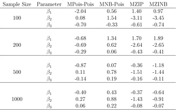
Table 2.1 shows that for all sample sizes (i.e., 100, 200, 500 and 1000), estimates of β1,
β2 and β3 from the MPois-Pois model have low biases when the true model is MPois-Pois,
and that the biases tend to decrease when the sample sizes increase. In these simulations, the MNB-Pois, MZIP and MZINB models also have low biases. From Table 2.2, it can be seen that the MPois-Pois model estimates Type I error rates for β1 close to 0.05, but that
MNB-Pois, MZIP and MZINB models tend to over-estimate the error rates when the true model is MPois-Pois. For such data, the MPois-Pois model estimated coverages of 95%
condence intervals for β1,β2 and β3 are in general close to the nominal value, particularly
MNB-Pois models converged, but convergence rates for the remaining marginalized models range from 88.0% to 90.2% for MNB-Pois, from 75.9% to 98.4% for MZIP, and from 72.0% to 96.6% for the MZINB models.
When the data are generated from Pois models, Table 2.5 shows that the MNB-Pois model gives low percent relative median biases forβ1,β2 andβ3, and the biases appear
to decrease as sample sizes increase. The corresponding estimates from the MZINB model also have low biases, but those from MPois-Pois and MZIP models are generally higher. In addition, the performance of the true MNB-Pois model with regard to Type I error rates (forβ1) and coverages of 95%condence intervals (forβ1,β2 andβ3) is superior to the other
three marginalized models (Tables 2.6 and 2.7, respectively) for larger sample sizes. Overall, the simulation results indicate that when the true model is MPois-Pois or MNB-Pois, the model estimates parameters with small biases, Type I errors close to the assumed rate and coverages of 95% condence intervals near 95% for large sample sizes.
2.6 Application to a Caries Incidence Trial
data is the large number of zero counts in the outcome variable, as 658 (19.28 %) of the
3412 children had zero DMFS counts (Figure 2.1). Since the number of zeros is much higher than what is expected under standard count probability mass functions (such as the Poisson and negative binomial), regression models based on these distributions may provide biased estimates and poor predictions. Marginalized models, however, account for zero-ination and enable the estimation of treatment eects on DMFS counts in the overall population.
We applied each of the two mixture distributions discussed in this article (i.e., Pois-Pois and NB-Pois mixtures) to model the marginal mean of DMFS. In each model, the marginal mean νi of DMFS and the mean parameter in a Poisson part of Pois-Pois and NB-Pois mixtures (i.e, µ1i) are related to the explanatory variables of interest as follows.
log(νi)=β0+β1bci+β2calci+β3bc_calci+β4N aFi+β5N aF T M Pi (2.53) log(µ1i)=ξ0+ξ1bci+ξ2calci+ξ3bc_calci
where bci is baseline caries from the ith child, calci is baseline calculus, bc_calci is the interaction ofbciandcalci,N aFi =1if the child was given sodium uoride, andN aF T M Pi =
1 if the child was randomized to the NaFTMP group with children in the SMFP group
making up the reference treatment category.
To model the mixing probability π and the reciprocal of the dispersion parameter α (for the NB-Pois model), only intercepts were specied using the logit and the negative log links, respectively.
logit(π)=ρ (2.54)
log(α)=−τ.
of excess zeros.
Table 2.9 summarizes the estimated log-likelihood and AIC values from the the four marginalized models together with incidence rate ratios for the NaF and NaFTMP groups relative to the SMFP group. The estimated regression coecients and standard errors for the marginal mean part of each of the four marginalized models are presented in Table 2.10. Based on the AIC criteria, the MNB-Pois (AIC=17192.9) provides the best t to the data compared to the other three models. The MZINB model has the next lowest AIC value and appears to give a good prediction of observed DMFS proportions as the MNB-Pois model (Figure 2.2).
Based on the best-tting model (i.e., MNB-Pois), the estimated incidence density ratio of a child in the NaF group is 0.942 CI (0.874, 1.015), relative to children with the same baseline status of caries and calculus who were assigned to SMFP. The corresponding incidence density ratio for children in the NaFTMP group is 0.970 CI (0.884, 1.063). Thus, children in the NaF and NaFTMP groups had a decrease in the marginal mean DMFS count by 5.5% and 3.0%, respectively, compared to children with the same baseline characteristics who were assigned to the SMFP group. However, the associations are not signicant since the condence intervals of the two incidence density ratios include 1.
2.7 Discussion
Table 2.1: Percent relative median biases of estimates of β1, β2 and β3 from marginalized
mixture models tted to data generated from the MPois-Pois model with 10,000 replications.
Sample Size Parameter MPois-Pois MNB-Pois MZIP MZINB
β1 -2.04 0.56 1.40 0.97
100 β2 0.08 1.54 -3.11 -3.45
β3 -0.70 -0.33 -0.61 -0.74
β1 -0.68 1.34 1.70 1.89
200 β2 -0.69 0.62 -2.64 -2.65
β3 -0.29 0.06 -0.43 -0.41
β1 -0.87 0.07 -0.36 -1.18
500 β2 0.11 0.78 -1.51 -1.44
β3 -0.14 0.19 -0.16 -0.11
β1 -0.40 0.43 -0.37 -0.64
1000 β2 0.27 0.88 -1.43 -0.91