Application of cluster analysis and multidimensional scaling on medical schemes data

Full text

(1)Application of Cluster Analysis and Multidimensional Scaling on Medical Schemes Data. by. Ian Roux. Thesis presented in partial fulfillment of the requirements for the degree of Master of Commerce at Stellenbosch University.. Department of Statistics and Actuarial Science Faculty of Economic and Management Sciences. Supervisor: Prof. N.J. Le Roux Date: December 2008. Co-supervisor: Prof. H. McLeod.

(2) ii. Declaration By submitting this thesis electronically, I declare that the entirety of the work contained therein is my own, original work, that I am the owner of the copyright thereof (unless to the extent explicitly otherwise stated) and that I have not previously in its entirety or in part submitted it for obtaining any qualification.. Date: 10 October 2008. Copyright © 2008 Stellenbosch University All rights reserved.

(3) iii. Summary Cluster analysis and multidimensional scaling (MDS) methods can be used to explore the structure in multidimensional data and can be applied to various fields of study. In this study, clustering techniques and MDS methods are applied to a data set from the health insurance field. This data set contains information of the number of medical scheme beneficiaries, between ages 55 to 59, that are treated for certain combinations of chronic diseases. Clustering techniques and MDS methods will be used to describe the interrelations among these chronic diseases and to determine certain clusters of chronic diseases. Similarity or dissimilarity measures between the chronic diseases are constructed before the application of MDS methods or clustering techniques, because the chronic diseases are binary variables in the data set. The calculation of dissimilarities between the chronic diseases is based on various dissimilarity coefficients, where a different dissimilarity coefficient will produce a different set of dissimilarities. One of the aims of this study is to compare different dissimilarity coefficients and it will be shown that the Jaccard, Ochiai, Baroni-Urbani-Buser, Phi and Yule dissimilarity coefficients are most suitable for use on this particular data set. MDS methods are used to produce a lower dimensional display space where the chronic diseases are represented by points and distances between these points give some measurement of similarity between the chronic diseases. The classical scaling, metric least squares scaling and nonmetric MDS methods are used in this study and it will be shown that the nonmetric MDS method is the most suitable MDS method to use for this particular data set. The Scaling by Majorizing a Complicated Function (SMACOF) algorithm is used to minimise the loss functions in this study and it was found to perform well. Clustering techniques are used to provide information about the clustering structure of the chronic diseases. Chronic diseases that are in the same cluster can be considered to be more similar, while chronic diseases in different clusters are more dissimilar. The robust clustering techniques: PAM, FANNY, AGNES and DIANA are applied to the data set. It was found that AGNES and DIANA performed very well on the data set, while PAM and FANNY performed only marginally well. The results produced by the MDS methods and clustering techniques are used to describe the interrelations between the chronic diseases, especially focussing on chronic diseases mentioned in the.

(4) iv same body system rule (Council for Medical Schemes, 2006, p.6-7). The cardiovascular diseases: Cardiomyopathy, Coronary Artery Disease, Dysrhythmias and Hypertension are strongly related to each other and to Asthma, Chronic Obstructive Pulmonary Disease, Diabetes Mellitus Type 2, Hypothyroidism and Hyperlipidaemia. The gastro-intestinal conditions: Crohn’s Disease and Ulcerative. Colitis seem to be very strongly related. Bipolar Mood Disorder, Epilepsy, Schizophrenia and Parkinson’s Disease also seem to be strongly related. The chronic diseases: Addison’s Disease and Diabetes Insipidus. also show a very strong relation to each other..

(5) v. Opsomming Trosontleding- en multidimensionele skalering (MDS) metodes kan gebruik word om die struktuur van multidimensionele data te ondersoek en kan in verskeie toepassingsgebiede aangewend word. Trosontleding- en MDS metodes gaan in hierdie studie op ’n datastel afkomstig uit die mediese skema bedryf toegepas word. Hierdie datastel bevat inligting oor die getal mediese skema lede, tussen die ouderdomme 55 en 59, wat behandeling ontvang vir sekere chroniese siektes. Die trosontledingen MDS tegnieke gaan gebruik word om verwantskappe tussen die chroniese siektes te beskryf.. Ongelyksoortigheidsmaatstawwe tussen die chroniese siektes moet eers bepaal word voordat die trosontledingen MDS tegnieke toegepas kan word, want die chroniese siektes is binêre veranderlikes in die datastel. Verskeie ongelyksoortigheidsmaatstawwe kan gebruik word in die praktyk. Verskillende ongelyksoortigheidsmaatstawwe mag egter verskillende resultate oplewer. Een van die doelwitte met hierdie studie is om verskeie ongelyksoortigheidsmaatstawwe te vergelyk en dit. is. bevind. dat. die. Jaccard,. Ochiai,. Baroni-Urbani-Buser,. Phi. en. Yule. ongelyksoortigheidsmaatstawwe die mees toepaslike vir gebruik op hierdie datastel is.. MDS metodes word gebruik in hierdie studie om ’n laer dimensionele figuur te produseer, waar die chroniese siektes as punte in die figuur voorgestel word en afstande tussen die punte ’n aanduiding verskaf van die gelyksoortigheid tussen die chroniese siektes. Klassieke skalering, metriese kleinste kwadrate skalering en nie-metriese MDS gaan in hierdie studie toegepas word. Dit is bevind dat die nie-metriese MDS metode die mees gepaste MDS metode is vir toepassing op hierdie datastel. Die “Scaling by Majorizing a Complicated Function” (SMACOF) algoritme word gebruik in hierdie studie om sekere verliesfunksies te minimeer en hierdie algoritme het baie bevredigend vertoon.. Trosontledingsmetodes word gebruik in hierdie studie om inligting oor die trosvorming van die chroniese siektes te verskaf. Chroniese siektes wat in dieselfde tros aangetref word, is meer soortgelyk, terwyl chroniese siektes in verskillende trosse weer meer van mekaar verskil. Die trosontledingsalgoritmes: PAM, FANNY, AGNES en DIANA word in hierdie studie toegepas op die datastel. Dit is bevind dat AGNES en DIANA baie goed vaar op die datastel, terwyl PAM en FANNY bevredigend vaar..

(6) vi Die resultate van die trosontledingen MDS tegnieke word gebruik om die verwantskappe tussen die chroniese siektes te beskryf, met spesiale klem wat geplaas word op chroniese siektes wat in dieselfde “body system rule” voorkom (Council for Medical Schemes, 2006, p.6-7). Daar is bevind dat die hartsiektes: “Cardiomyopathy”, “Coronary Artery Disease”, “Dysrhythmias” en “Hypertension” sterk verwant is aan mekaar en aan “Asthma”, “Chronic Obstructive Pulmonary Disease”, “Diabetes Mellitus Type 2”, “Hypothyroidism” en “Hyperlipidaemia”. Dit lyk ook of “Crohn’s Disease” en “Ulcerative. Colitis” baie nou verwant is aan mekaar. “Bipolar Mood Disorder”, “Epilepsy”, “Schizophrenia” en “Parkinson’s Disease” vertoon ook ’n sterk verwantskap. Verder lyk dit ook of “Addison’s Disease” en “Diabetes Insipidus” baie nou verwant is aan mekaar..

(7) vii. Acknowledgements •. I would like to thank Prof. N.J. Le Roux, my supervisor, for his constant encouragement and invaluable guidance.. •. I also would like to thank Prof. Heather McLeod, my co-supervisor, for her help and efforts to make the data set available.. •. I want to thank the following members of the REF Study 2005 Consortium: André Deetlefs, Andre Meyer, Brett Mill and Pierre Robertson for their efforts to make the data available.. •. I would like to thank Old Mutual Healthcare (Pty) Ltd., Medscheme (Pty) Ltd., Discovery Health (Pty) Ltd. and Metropolitan Health Group (Pty) Ltd. for providing the data.. •. I would like to thank the Harry Crossley foundation for their funding.. •. I want to thank all my friends, especially those living at 15 Karee Street, for their friendship and support.. •. I want to thank the Gertenbach’s on Belvedere farm for their hospitality, support and encouragement.. •. I would like to thank Alechia for her love, friendship and constant support throughout my studies.. •. Finally, but most significantly, I want to thank my parents for their encouragement, love and support throughout my studies and throughout my life..

(8) viii. Contents Declaration. ii. Summary. iii. Opsomming. v. Acknowledgements. vii. Contents. viii. Chapter 1: Introduction. 1. 1.1. Introduction. 1. 1.2. The REF Entry and Verification Criteria and the Body System Rules. 3. 1.3. The Medical Scheme 55-59 Data Set. 5. 1.4. Aims of this Study. 8. 1.5. Methods used in this Study. 9. 1.6. Notation and Abbreviations. 10. 1.7. Definitions and Terminology used in this Study. 11. Chapter 2: Description of the Medical Scheme 55-59 Data Set. 12. 2.1. Introduction. 12. 2.2. Univariate Description of the Medical Scheme 55-59 Data Set. 12. 2.3. Summary. 29. Chapter 3: Calculating Proximities between the Chronic Diseases. 31. 3.1. Introduction. 31. 3.2. Construction of Similarity and Dissimilarity Coefficients for Binary Data. 32. 3.3. Metric and Euclidean Properties of Dissimilarity Coefficients for Binary Data. 34. 3.4. Calculation of Dissimilarities between the Chronic Diseases. 36. 3.5. Summary. 39.

(9) ix. Chapter 4: Displaying the Relationships between Chronic Diseases using MDS Techniques. 40. 4.1. Introduction. 40. 4.2. Multidimensional Scaling Methods used in this Study. 41. 4.2.1. Metric multidimensional scaling. 41. 4.2.1.1. Classical scaling. 41. 4.2.1.2. Metric least square scaling. 43. 4.2.2 4.3. Nonmetric multidimensional scaling Application of the MDS Methods to the Medical Scheme 55-59 Data Set. 4.3.1. Metric multidimensional scaling. 47 50 50. 4.3.1.1. Classical scaling. 50. 4.3.1.2. Metric least square scaling. 58. 4.3.2 4.4. Nonmetric multidimensional scaling. 65. Application of the Nonmetric MDS Method to the Male MS (55-59) and. 4.5. Female MS (55-59) Data Sets. 78. Summary. 83. Chapter 5: Clustering of the Chronic Diseases using the Algorithms of Kaufman & Rousseeuw. 87. 5.1. Introduction. 87. 5.2. Input Structures for Cluster Analysis. 88. 5.3. The Clustering Algorithms of Kaufman and Rousseeuw. 89. 5.3.1. Partitioning methods. 89. 5.3.1.1. Partitioning around medoids (PAM). 89. 5.3.1.2. Clustering large applications (CLARA). 92. 5.3.1.3. Fuzzy Analysis (FANNY). 93. 5.3.2. Hierarchical methods. 95. 5.3.2.1. Agglomerative nesting (AGNES). 95. 5.3.2.2. Divisive analysis (DIANA). 97. 5.3.2.3. Monothetic analysis (MONA). 99.

(10) x 5.4. Application of the Clustering Techniques on the Medical Scheme 55-59 Data Set. 100. 5.4.1. Choice of clustering techniques. 100. 5.4.2. Application of AGNES. 101. 5.4.3. Application of DIANA. 109. 5.4.4. Application of PAM. 114. 5.4.5. Application of FANNY. 124. 5.5. Application of the Clustering Techniques on the Male MS (55-59) and Female MS (55-59) Data Sets. 132. 5.5.1. Application of AGNES. 133. 5.5.2. Application of DIANA. 135. 5.5.3. Application of PAM. 137. 5.5.4. Application of FANNY. 140. 5.6. Summary. 143. Chapter 6: Conclusions. 147. Appendix A. 153. Appendix B. 175. References. 176.

(11) 1. Chapter 1 Introduction 1.1. Introduction. Consider a data set consisting of p variables measured for each of n objects. Well-known visual displays, like scatterplots for example, can be used to explore the data if p = 2 or 3. However, it becomes more difficult to display the relationships among the objects, the relationships among the variables or the variable-object relationships when p becomes larger than three. Multidimensional scaling (MDS) and cluster analysis are two statistical techniques that can be used to explore the structure of multidimensional data. Although both clustering techniques and MDS methods are used to describe how the objects or variables in a certain data set are related, the two approaches are different. Borg & Groenen (2005) describe MDS as a “method that represents measurements of similarity (dissimilarity) between objects as distances between points in a lower dimensional space”. For example, points in this lower dimensional (usually two dimensional) space that lie close to one another indicate that the corresponding objects have a greater similarity. The objects are not classified into clusters, but distances between the points can be used to assess the relationships among the objects. However, the interpretation of the distances is rather subjective, as different observers might reach different conclusions with regard to possible clusters. Furthermore, it is impossible to capture all the variability of the multidimensional data in a lower dimensional display. Clustering techniques, on the other hand, produce information about the clustering structure of the objects. Anderberg (1973) mentions that “the objective of the clustering techniques is either to group data objects or the variables into clusters, in such a way that the elements belonging to the same cluster resemble each other, whereas elements in different clusters are dissimilar” . The clustering structure found is based on actual similarity measurements between the objects. Clustering techniques are also well suited to high dimensional data. One of the possible drawbacks of clustering techniques is that it can be difficult to interpret the relationships among the objects. For example, many clustering methods only produce a list of clusters and their objects as output that might be difficult to interpret. However, certain visual displays have been developed to overcome this drawback, and are known as clusplots (Pison et al., 1998). Clusplots use MDS to produce a.

(12) 2 configuration of points in a two dimensional display and use clustering techniques to find a clustering structure. The clusters are then represented by ellipses in the lower dimensional display. Clusplots illustrate that it is useful to supplement MDS configurations with information about the clustering structure of the objects. However, clusplots do not usually use the correct aspect ratio. This means that a unit change in the horizontal direction of the graphical display is not equal to a unit change in the vertical direction and distances between objects in the graphical display can therefore not be fully appreciated, which is vital for interpretation. Care must therefore be taken by the user when implementing clusplots to ensure that the correct aspect ratio is used. Another limitation of clusplots is that clusplots do not provide information about the variables when the objects are clustered. Biplots (Gower & Hand, 1996) can be used to overcome this limitation by providing a graphical display with information on both the objects and the variables simultaneously. Cluster analysis and MDS methods are applied to various fields including medical research, ecology, economics, psychometrics, chemometrics, and many more (Kaufman & Rousseeuw, 1990). It will be shown that the clustering techniques and MDS methods can also be used on a South African data set in the health insurance field. This data set is known as the REF Study 2005 raw data set and it was provided by the Risk Equalisation Fund (REF) Study 2005 consortium. The REF will equalise risk with regard to the age and disease profile of medical scheme beneficiaries in South Africa in relation to the Prescribed Minimum Benefit (PMB) conditions (Council for Medical Schemes, 2005, p.1). Risk equalisation is not unique to South Africa and has been introduced by many countries that include: Belgium, Finland, Germany, Czech Republic, Germany, Ireland, Netherlands, Norway, Russian Federation, Sweden, Switzerland, United Kingdom, Israel, Australia, New Zealand, Colombia, Canada and the United States of America (Parkin & McLeod, 2001). The REF Study 2005 raw data set was collected from four major medical scheme administrators in South Africa in order to produce the REF Contribution Table 2007 (RETAP, 2007). These four administrators provided services to approximately 4.25 million beneficiaries, which represented approximately 63% of South Africa’s total medical scheme beneficiaries reported in 2005 (RETAP, 2007, p.16). The data set contains information about the costs and exposure for unique combinations of age, gender and disease, where the exposure is measured in beneficiary months. There are 19 different age bands and 25 REF chronic diseases. It is important to investigate how the chronic diseases are related to one another, where a strong relationship between two chronic diseases indicates that they tend to co-occur often. Results from such an investigation could confirm medical.

(13) 3 knowledge of relationships among certain chronic diseases. Also, the results could be used if the REF Entry and Verification Criteria, with regard to multiple chronic diseases, are changed in the future. The REF Entry and Verification Criteria will be discussed in Section 1.2. Scatterplots and histograms cannot be used to display the relationships among all the chronic diseases simultaneously, because the REF Study 2005 raw data set is multidimensional. It is therefore necessary to use MDS methods or clustering techniques to display the relationships among the chronic diseases, and it will be shown that these methods are well suited to this purpose. Both MDS methods and clustering techniques will be used, as Gordon (1999) points out that “such combined analyses will reduce the element of subjectivity in assessing results. If similar conclusions would be reached from the separate analyses, one can have more confidence in the accuracy of the results.” 1.2. The REF Entry and Verification Criteria and the Body System Rules. Medical schemes in South Africa have to submit monthly data to the REF on a quarterly basis. The data that medical schemes submit to the REF are in the form of REF Grid Count data (Council for Medical Schemes, 2006). A medical scheme will then either receive or make a payment to the REF, dependent on this REF Grid Count data. The payments will depend on the age, gender of the beneficiaries and the number of beneficiaries treated for a certain chronic disease. The type of chronic disease and the number of multiple chronic diseases will also influence the payments. It is therefore important that the REF enforces strict Entry and Verification Criteria of the data submitted, to ensure a fair system. Note however that the REF is not yet in full operation, and currently operates in a “shadow period” where medical schemes submit data but no money actually changes hands (RETAP, 2007). There was a change in the REF Entry and Verification Criteria, applicable to all medical scheme administrators from 1 January 2007 (Council for Medical Schemes, 2006, p.6-7) and known as the REF Entry and Verification Criteria version 2. The change regards the following eight rules, which will be called body system rules in this study. These rules will affect the REF Grid Count data if beneficiaries are treated for certain multiple chronic diseases. The body system rules are the following:.

(14) 4 1.. For Count purposes, only one of the following chronic respiratory diseases can be assigned to the same beneficiary: Chronic Obstructive Pulmonary Disease, Asthma and Bronchiectasis (COP, AST or BCE).. 2.. For Count purposes, only one of the following cardiovascular diseases can be assigned to the same beneficiary: Cardiomyopathy, Coronary Artery Disease, Dysrhythmias and Hypertension (CMY, IHD, DYS or HYP).. 3.. For Count purposes, only one of Hypertension or Chronic Renal Failure can be assigned to the same beneficiary (HYP or CRF).. 4.. For Count purposes, only one of the following gastro-intestinal conditions can be assigned to the same beneficiary: Crohn’s disease and Ulcerative Colitis (CSD or IBD).. 5.. For Count purposes, only one of Bipolar Mood Disorder and Schizophrenia can be assigned to the same beneficiary (BMD or SCZ).. 6.. For Count purposes, only one of Multiple Sclerosis, Bipolar Mood Disorder and Epilepsy can be assigned to the same beneficiary (MSS, BMD or EPL).. 7.. For Count purposes, only one of Systemic Lupus Erythematosus and Rheumatoid Arthritis can be assigned to the same beneficiary (SLE or RHA).. 8.. Diabetes Mellitus Type 1 and Type 2 cannot co-occur.. Various chronic diseases mentioned in the same body system rule present clinical diagnostic challenges in the absence of convincing clinical evidence (RETAP, 2007, p.74). The body system rules will prevent over counting of these chronic diseases and will help to ensure a fair system. An important distinction is made between whether a life (defined as a beneficiary month) is treated for a certain disease or diagnosed with a certain disease, with treated being the more strict criterion. A life is treated for a certain disease when the life meets the REF Entry and Verification criteria version 2 (Council for Medical Schemes, 2006, p.19-35). The REF Entry and Verification criteria.

(15) 5 version 2 require specific diagnosis-related information and proof of treatment for each of the REF chronic diseases and HIV, before the life can be classified as a “treated patient”. The REF Study 2005 raw data set is based on the REF Entry and Verification criteria version 2 for CDL (chronic disease list) conditions (Council for Medical Schemes, 2006, p.19-35) and known as TREATED data (RETAP, 2007, p.18). The chronic disease list is a list of 25 chronic diseases as prescribed in the Amendment to the General Regulations made in terms of the Medical Scheme Act of 1998, (Act 131 of 1998, p.35). It must be noted that the last body system rule was actually applied to the TREATED REF Study 2005 raw data set. The REF Entry and Verification criteria version 2 state that “for REF purposes, Type 1 and Type 2 diabetes cannot occur concurrently. Evidence of use of oral euglycaemic or hypoglycaemic medicines automatically leads to the classification of a diabetic case as Type 2.” (Council for Medical Schemes, 2006, p.26). The Diabetes Mellitus Type 1 and Type 2 chronic diseases therefore do not show any co-occurrence in the TREATED REF Study 2005 raw data set. The other body system rules were not applied to the TREATED REF Study 2005 raw data set. 1.3. The Medical Scheme 55-59 Data Set. MDS methods and clustering techniques will be used to describe the relationships among the chronic diseases, which are binary variables in the TREATED REF Study 2005 raw data set. However, the application of the MDS methods and clustering techniques on the TREATED REF Study 2005 raw data set is not a straightforward task. Firstly, measurements of similarity (dissimilarity) between the binary variables must be calculated and there are at least 43 possible similarity coefficients that could be used (Hubàlek, 1982). The choice of similarity coefficient is very important as it will heavily influence the graphical displays produced by the MDS methods and clustering techniques. Some of these similarity coefficients will be more appropriate to use than others, depending on the actual data set. Cox & Cox (2001) recommend using several different similarity coefficients in practice, hoping for robustness against a specific choice. Secondly, several MDS methods can be applied to the data set and these methods will produce different configurations of points in the graphical displays. Several clustering techniques can also be used, and these techniques will also produce different clustering structures. Gordon (1999) mentions.

(16) 6 that it is rarely the case that only one method of analysis is particularly appropriate for a certain study. It therefore seems more appropriate to use several MDS methods and several clustering techniques, and not just a single method. “Different age bands have different disease profiles, with multiple conditions becoming more apparent later in life” (Council for Medical Schemes, 2005, p.26). This means that MDS methods and clustering techniques are very likely to produce different results for the different age bands. Therefore, it is important to produce results according to particular age bands. This study will focus only on one of these age bands, as it is not practical to repeat the same methodology for all 19 age bands, remembering that the methodology will depend on several similarity coefficients, several MDS methods and several clustering techniques. However, other age bands can be analysed in a similar way in future. According to McLeod (2007), leader of the REF Study 2005 consortium, the age band of 55 to 59 years contains the most lives treated for chronic diseases, out of all 19 age bands, in the TREATED REF Study 2005 raw data set. This age band also shows the occurrence of every single chronic disease and many of these chronic diseases co-occur, which makes this a suitable age band to use when describing the relationships among the chronic diseases. The Medical Scheme 55-59 data set is a subset of the TREATED REF Study 2005 raw data set, where only the age band of 55 to 59 years is considered. The results from the complete analysis of this particular age band can be used to determine which choices of various similarity coefficients, MDS methods and clustering techniques are more appropriate, and these results can then be used if similar analyses of the other age bands are carried out in future. Still, the use of only one age band in this study has the drawback that the important relationship between age and chronic disease cannot be explored. The variables of the Medical Scheme 55-59 data set used in this study, along with the respective codes, are given in Table 1.1. The REF chronic diseases and HIV are binary variables where “1” indicates that the lives are treated for the corresponding disease and “0” indicates that the lives are not treated for the particular disease. The variable NON is also a binary variable where “1” indicates that the lives are not treated for any of the 25 REF chronic diseases or HIV and the lives are not claiming for maternity benefits. The variable Nr.Lives indicates the number of lives that are treated for the same combination of diseases. This means that each row of the Medical Scheme 55-59 data set represents multiple identical lines of individual lives that are treated for the same unique combination of diseases. The last three variables are continuous variables that measure the average.

(17) 7 Table 1.1:. Variables of the Medical Scheme 55-59 data set that will be used in this study.. Codes. Description. NON. Not treated for any chronic disease or HIV, and no maternity benefit was claimed.. ADS. Addison’s Disease. AST. Asthma. BCE. Bronchiectasis. BMD. Bipolar Mood Disorder. CMY. Cardiomyopathy. COP. Chronic Obstructive Pulmonary Disease. CRF. Chronic Renal Failure. CSD. Crohn’s disease. DBI. Diabetes Insipidus. DM1. Diabetes Mellitus Type 1. DM2. Diabetes Mellitus Type 2. DYS. Dysrhythmias. EPL. Epilepsy. GLC. Glaucoma. HAE. Haemophilia. HYL. Hyperlipidaemia. HYP. Hypertension. IBD. Ulcerative Colitis. IHD. Coronary Artery Disease. MSS. Multiple Sclerosis. PAR. Parkinson’s Disease. RHA. Rheumatoid Arthritis. SCZ. Schizophrenia. SLE. Systemic Lupus Erythematosus. TDH. Hypothyroidism. HIV. HIV/AIDS. Nr.Lives. Number of lives that have the same gender and disease combination. Hospital. Average DTP Hospital costs. Medicine. Average CDL Medicine costs. Related. Average Total Related costs.

(18) 8 cost for each combination of chronic diseases that were treated. The average cost is described in three categories: DTP Hospital cost, CDL Medicine cost and Total Related cost. The Total Related costs in the REF Study 2005 were defined to be the sum of DTP Related costs, CDL Related costs and Capitation costs (RETAP, 2007, p.28). Appendix B contains the first 30 rows of the Medical Scheme 55-59 data set. The Male MS (55-59) data set and Female MS (55-59) data set are two subsets of the Medical Scheme 55-59 data set, reflecting male and female lives. These two data subsets will be used to describe differences between male and female lives, with regard to the occurrence of chronic diseases. 1.4. Aims of this Study. MDS methods and clustering techniques will be applied to the Medical Scheme 55-59 data set, where an attempt will be made to describe the relationships among the 25 REF chronic diseases, HIV and NON. Chronic diseases and HIV that co-occur more often in the Medical Scheme 55-59 data set are expected to show a stronger relationship in the MDS and clustering graphical displays. The results produced by these methods can then be used to investigate whether chronic diseases mentioned in the same body system rule are strongly related. It is also important to investigate which other chronic diseases, not mentioned in the body system rules, also have strong relationships. Differences between male and female lives with regard to the occurrence of chronic diseases also need to be investigated. MDS methods can be used to produce separate displays for male and female lives where points in these displays represent the various chronic diseases. Clustering techniques can also be used to produce separate displays for male and female lives, where these displays will show the clustering structures of the chronic diseases. These graphical displays will be used to describe differences between male and female lives. This study will only focus on the 55-59 year age band and several similarity coefficients, several MDS methods and several clustering techniques will be used. The results from the study, for this particular age band, can then be used to determine which choices of similarity coefficient, MDS method and clustering technique are more appropriate to use for other age bands, should a similar analysis of the other age bands be carried out in the future..

(19) 9 1.5. Methods used in this Study. All of the statistical techniques used in this study were carried out by using the programming and graphical environment of the computer package R, available from http://www.cran.rproject.org. Some of the standard R functions were used in this study. Also, several new functions were constructed for use in this study. Details of these functions are provided in Appendix A. The Medical Scheme 55-59 data set will be discussed in detail in Chapter 2. Histograms and tables will be used to describe the cost aspects and the occurrence of the various chronic diseases. The calculation of dissimilarities between binary variables, based on several similarity coefficients, will be discussed in Chapter 3. These dissimilarities will provide some measurement of how similar (dissimilar) chronic diseases are to each other. The dissimilarities will be used in Chapter 4 and Chapter 5, where an attempt will be made to display the different chronic diseases. Some metric and Euclidean properties of the various dissimilarity coefficients will also be discussed in Chapter 3. The metric and Euclidean properties of these dissimilarity coefficients are important to consider when the chronic diseases are displayed in Chapters 4 and 5 (Gower & Legendre, 1986). Some of these displays will only be appropriate to use if certain metric requirements are met. Metric and nonmetric MDS methods will be discussed in Chapter 4. The main difference between metric and nonmetric MDS methods is that metric MDS methods require dissimilarity coefficients with metric properties and nonmetric MDS methods only use the ranking order of the dissimilarities and can therefore accept dissimilarity coefficients with or without metric properties. However, the display space for both metric and nonmetric MDS methods will be chosen to be Euclidean. This means that the displays will have a direct distance-like interpretation. Points representing chronic diseases that lie close to each other indicate that these chronic diseases tend to co-occur often. Nonmetric MDS methods produce graphical displays where the configuration of points is determined by minimising a certain loss function. Scaling by Majorizing a Complicated Function (SMACOF) is a technique that was developed to minimise complicated functions and will be used in this study to minimise loss functions. It will be shown how SMACOF can be used for nonmetric and metric MDS methods (Borg & Groenen, 2005). The performance of metric and nonmetric MDS methods, in the case of the Medical Scheme 55-59 data set, will also be compared. This will be discussed in Chapter 4..

(20) 10 Chapter 5 is concerned with the cluster analysis of the Medical Scheme 55-59 data set, where clustering structures of the chronic diseases will be produced. This study will focus on the robust clustering algorithms of Kaufman & Rousseeuw (1990), as these clustering algorithms are very well suited to analysing the Medical Scheme 55-59 data set. The graphical representations accompanying the Kaufman and Rousseeuw algorithms, showing the clustering structures of the chronic diseases, are of particular importance. These clustering structures group the REF chronic diseases, HIV and NON into clusters, in such a way that the diseases belonging to the same cluster resemble each other, whereas diseases in different clusters are dissimilar. The clusplot graphical display (Pison et al., 1998) will also be discussed. The dissimilarities between chronic diseases calculated in Chapter 3, will be used as input structures for the clustering algorithms. It is important to consider the performance of the various similarity (dissimilarity) coefficients. The performance of the clustering algorithms of Kaufman & Rousseeuw will also be compared to the more traditional clustering methods. 1.6. Notation and Abbreviations. x. Scalar. X. Random variable. x. Column vector T. X. The transpose of matrix X. xT. The transpose of vector x. X: n × p. A matrix consisting of n rows and p columns. In. Identity matrix with n rows and n columns. sij. Similarity coefficient between objects i and j. dij. Dissimilarity coefficient between objects i and j. δij. Distance between objects i and j in the lower dimensional display space. s(i). Silhouette value of object i. L. The best fitting r-dimensional subspace. SVD. Singular value decomposition. MDS. Multidimensional scaling. PCA. Principal component analysis. SMACOF. Scaling by majorizing a complicated function. PAM. Partitioning around medoids. CLARA. Clustering large applications.

(21) 11 FANNY. Fuzzy clustering. AGNES. Agglomerative nesting. DIANA. Divisive analysis. MONA. Monothetic analysis. AC. Agglomerative coefficient. DC. Divisive coefficient. REF. Risk Equalisation Fund. 1.7. Definitions and Terminology used in this Study. CDL. Chronic disease list conditions, which is a list of 25 chronic diseases as prescribed in the Amendment to the General Regulations made in terms of the Medical Scheme Act of 1998, (Act 131 of 1998, p.35).. Chronic disease. A disease that is listed as a CDL.. Age. Age last birthday on 1 January.. Life. A single beneficiary month.. Treated patient. Patient that is treated for a certain disease, which means that the patient meets the REF Entry and Verification criteria version 2 for CDL conditions (Council for Medical Schemes, 2006, p.19-35). The REF Entry and Verification criteria version 2 require specific diagnosis-related information and proof of treatment for each of the chronic diseases and HIV.. TREATED data. Data based on the REF Entry and Verification criteria version 2 for CDL conditions.. Medical Scheme 55-59 data A subset of the TREATED REF Study 2005 raw data set provided by the REF Study 2005 consortium. This subset contains information regarding the average costs and the number of lives treated for unique combinations of gender and disease, where the lives are 55 to 59 years old. Male MS (55-59) data set. A subset of the Medical Scheme 55-59 data set, containing male lives.. Female MS (55-59) data set A subset of the Medical Scheme 55-59 data set, containing only female lives..

(22) 12. Chapter 2 Description of the Medical Scheme 55-59 Data Set 2.1. Introduction. The Medical Scheme 55-59 data set, introduced in Chapter 1, will be described further in this chapter by using univariate statistical techniques. Histograms and tables will be used to describe the occurrence of the chronic diseases and the costs of treatment. 2.2. Univariate Description of the Medical Scheme 55-59 Data Set. The Medical Scheme 55-59 data set contains 1 636 rows of unique combinations of gender and disease and represents 2 199 367 lives. The Male MS (55-59) data set contains 750 rows of unique combinations of disease and represents 1 056 917 male lives. The Female MS (55-59) data set contains 886 rows and represents 1 142 450 female lives. Table 2.1 contains the number of male and female lives that were treated for certain chronic diseases. Most of the lives in the Medical Scheme 55-59 data set were not treated for any of the chronic diseases or HIV. Observe from Table 2.1 that the chronic diseases HAE, DBI, ADS, BCE and MSS did not occur often, while the chronic diseases AST, TDH, DM2, HYL and HYP occurred more often. A similar observation was made for the 2002 data where HYP, HYL and AST were found to be some of the most common chronic diseases (Council for Medical Schemes, 2005, p.37). Observe from Table 2.1 that there is a difference between the number of male and female lives treated for certain diseases, but a direct comparison cannot easily be made because the total number of male and female lives in the Medical Scheme 55-59 data set are different. It is therefore more convenient to use chronic disease rates to make a direct comparison between male and female lives. RETAP (2007) used a “chronic rate per 1,000 lives”. The chronic disease rate that will be used in this study is defined in Definition 2.1. Definition 2.1 Chronic disease rate The number of lives per 1 000 that are treated for a certain chronic disease, where lives are defined as beneficiary months. (For example, a female treated for HAE for four months is counted as four female lives.).

(23) Table 2.1:. 13 The number of male and female lives treated for a certain chronic disease. Many. lives are treated for multiple chronic diseases. The number of lives that are not treated for any chronic disease or HIV, coded as NON, is also provided. Variables. Male. Female. Total. HAE. 0. 4. 4. DBI. 21. 53. 74. ADS. 116. 91. 207. MSS. 19. 215. 234. BCE. 156. 326. 482. CSD. 362. 329. 691. SLE. 140. 631. 771. SCZ. 356. 772. 1 128. CRF. 1 094. 598. 1 692. IBD. 897. 808. 1 705. PAR. 1 029. 703. 1 732. BMD. 802. 1 226. 2 028. HIV. 2 451. 1 236. 3 687. GLC. 3 984. 4 716. 8 700. DYS. 5 321. 4 043. 9 364. DM1. 7 050. 4 386. 11 436. EPL. 5 954. 6 252. 12 206. COP. 7 215. 6 396. 13 611. RHA. 4 401. 11 423. 15 824. CMY. 13 120. 11 229. 24 349. IHD. 28 615. 13 887. 42 502. AST. 20 169. 30 328. 50 497. TDH. 7 498. 61 755. 69 253. DM2. 49 123. 34 066. 83 189. HYL. 104 036. 68 270. 172 306. HYP. 196 341. 224 680. 421 021. NON. 763 387. 813 432. 1 576 819. Total. 1 056 917. 1 142 450. 2 199 367.

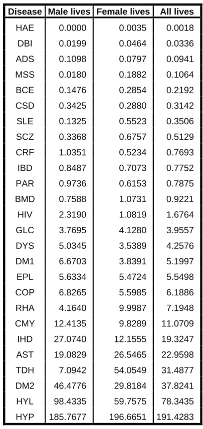
(24) 14 Table 2.2:. Chronic disease rates (see Definition 2.1) of the Medical Scheme 55-59 data set. Disease Male lives Female lives. All lives. HAE. 0.0000. 0.0035. 0.0018. DBI. 0.0199. 0.0464. 0.0336. ADS. 0.1098. 0.0797. 0.0941. MSS. 0.0180. 0.1882. 0.1064. BCE. 0.1476. 0.2854. 0.2192. CSD. 0.3425. 0.2880. 0.3142. SLE. 0.1325. 0.5523. 0.3506. SCZ. 0.3368. 0.6757. 0.5129. CRF. 1.0351. 0.5234. 0.7693. IBD. 0.8487. 0.7073. 0.7752. PAR. 0.9736. 0.6153. 0.7875. BMD. 0.7588. 1.0731. 0.9221. HIV. 2.3190. 1.0819. 1.6764. GLC. 3.7695. 4.1280. 3.9557. DYS. 5.0345. 3.5389. 4.2576. DM1. 6.6703. 3.8391. 5.1997. EPL. 5.6334. 5.4724. 5.5498. COP. 6.8265. 5.5985. 6.1886. RHA. 4.1640. 9.9987. 7.1948. CMY. 12.4135. 9.8289. 11.0709. IHD. 27.0740. 12.1555. 19.3247. AST. 19.0829. 26.5465. 22.9598. TDH. 7.0942. 54.0549. 31.4877. DM2. 46.4776. 29.8184. 37.8241. HYL. 98.4335. 59.7575. 78.3435. HYP. 185.7677. 196.6651. 191.4283.

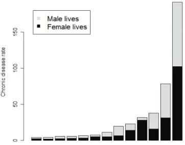
(25) 15 For example, the female HAE chronic disease rate is calculated as follows from Table 2.1: Number of female lives treated for HAE Total number of all female lives. × 1000 =. 4 × 1000 = 0.0035 1 142 450. Table 2.2 contains the chronic disease rates of male and female lives of the Medical Scheme 55-59 data set. The values in Table 2.2 show that male and female chronic disease rates differ dramatically for some chronic diseases. For example, the chronic disease MSS occurred 10 times more often in female lives. The chronic disease rates are graphically displayed in Figures 2.1 and 2.2. It can be observed from Figure 2.1 and Figure 2.2 that female lives have much higher chronic disease rates for DBI, MSS, BCE, SLE, SCZ, BMD, RHA and TDH, while the male lives have higher chronic disease rates for CRF, PAR, IHD and HYL. The chronic disease with the highest chronic disease rate is HYP.. Figure 2.1:. Chronic disease rates of chronic diseases that occurred least often. The breakdown. for male and female lives is also displayed. See Definition 2.1..

(26) 16. Figure 2.2:. Chronic disease rates of chronic diseases that occurred most often.. Some lives are not treated for any chronic diseases, others for a single chronic disease, while others are treated for multiple chronic diseases. Table 2.3 shows the number of lives that are treated for a certain number of chronic diseases. It can be observed from Table 2.3 that approximately 72% of all lives are not treated for any chronic disease. Approximately 17% of all lives are only treated for one chronic disease. Table 2.3:. Number and percentage of male and female lives that were treated for a certain. number of chronic diseases.. Number of chronic diseases (including HIV). Male lives Female lives Male percentage Female percentage. None. 763 387. 813 432. 72.2277. 71.2007. 1. 174 065. 210 677. 16.4691. 18.4408. 2. 82 491. 86 171. 7.8049. 7.5426. 3. 28 564. 25 002. 2.7026. 2.1885. 4. 6 839. 5 718. 0.6471. 0.5005. 5. 1 300. 1 205. 0.1230. 0.1055. 6. 225. 214. 0.0213. 0.0187. 7. 43. 31. 0.0041. 0.0027. 8. 3. 0. 0.0003. 0.0000.

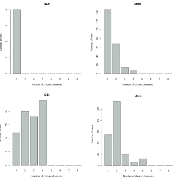
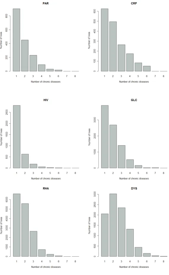
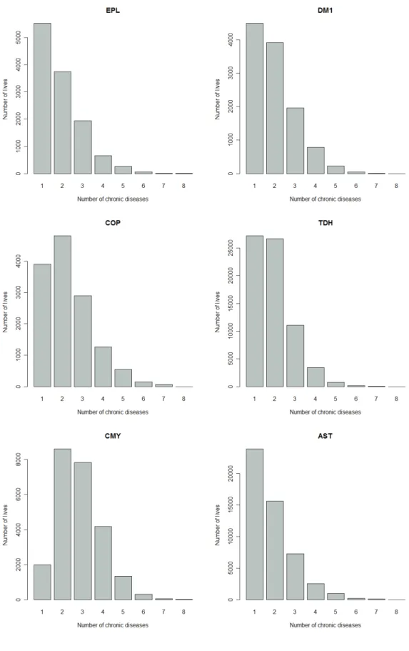
(27) 17. Figure 2.3:. Number of lives treated for a particular chronic disease and also treated for none,. one, two, three, …, seven other chronic diseases. The number of lives corresponding to 1 is the number of lives treated only with one particular chronic disease. The number of lives corresponding to 2 is the number of lives that are treated for the particular chronic disease and only one other chronic disease..

(28) 18. Figure 2.3:. Continued..



(31) 21. Figure 2.3:. Continued.. Figure 2.3 gives a breakdown of the number of lives treated for 1, 2, 3, …, 8 chronic diseases, where the breakdown is done for each chronic disease. This will give information about the co-occurrences of certain diseases. It can be observed from Figure 2.3 that CMY, IHD, DM2, HYL, DYS, BCE, SLE, ADS and DBI tend to co-occur often with other chronic diseases, while the chronic diseases MSS, PAR, HIV and HAE show much less co-occurrence with other chronic diseases. The histograms in Figure 2.3 provide information about the co-occurrences of certain chronic diseases, but the usefulness of these histograms is limited. The histograms show that some chronic diseases, like CMY, co-occur often with other chronic diseases, but with which diseases do CMY co-occur? The histograms do not show which of the chronic diseases are strongly related..

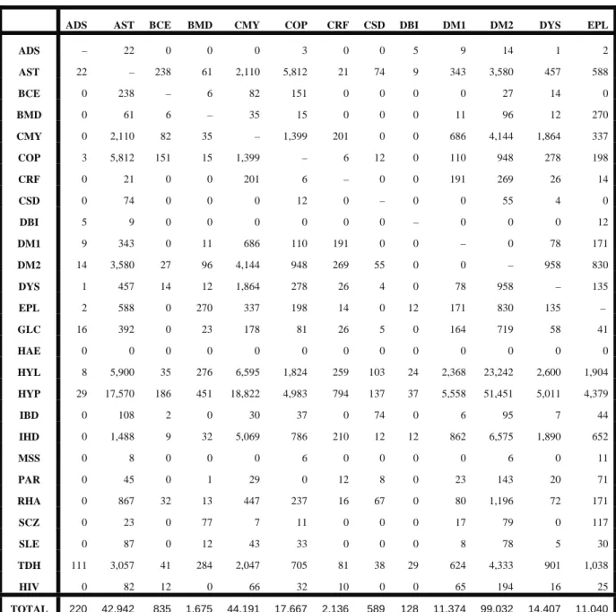
(32) 22 Table 2.4:. Number of co-occurrences between pairs of chronic diseases. ADS. AST. BCE. BMD. CMY. COP. CRF. CSD. DBI. DM1. DM2. DYS. EPL. ADS. –. 22. 0. 0. 0. 3. 0. 0. 5. 9. 14. 1. 2. AST. 22. –. 238. 61. 2,110. 5,812. 21. 74. 9. 343. 3,580. 457. 588. BCE. 0. 238. –. 6. 82. 151. 0. 0. 0. 0. 27. 14. 0. BMD. 0. 61. 6. –. 35. 15. 0. 0. 0. 11. 96. 12. 270. CMY. 0. 2,110. 82. 35. –. 1,399. 201. 0. 0. 686. 4,144. 1,864. 337. COP. 3. 5,812. 151. 15. 1,399. –. 6. 12. 0. 110. 948. 278. 198. CRF. 0. 21. 0. 0. 201. 6. –. 0. 0. 191. 269. 26. 14. CSD. 0. 74. 0. 0. 0. 12. 0. –. 0. 0. 55. 4. 0. DBI. 5. 9. 0. 0. 0. 0. 0. 0. –. 0. 0. 0. 12. DM1. 9. 343. 0. 11. 686. 110. 191. 0. 0. –. 0. 78. 171. DM2. 14. 3,580. 27. 96. 4,144. 948. 269. 55. 0. 0. –. 958. 830. DYS. 1. 457. 14. 12. 1,864. 278. 26. 4. 0. 78. 958. –. 135. EPL. 2. 588. 0. 270. 337. 198. 14. 0. 12. 171. 830. 135. –. GLC. 16. 392. 0. 23. 178. 81. 26. 5. 0. 164. 719. 58. 41. HAE. 0. 0. 0. 0. 0. 0. 0. 0. 0. 0. 0. 0. 0. HYL. 8. 5,900. 35. 276. 6,595. 1,824. 259. 103. 24. 2,368. 23,242. 2,600. 1,904. HYP. 29. 17,570. 186. 451. 18,822. 4,983. 794. 137. 37. 5,558. 51,451. 5,011. 4,379. IBD. 0. 108. 2. 0. 30. 37. 0. 74. 0. 6. 95. 7. 44. IHD. 0. 1,488. 9. 32. 5,069. 786. 210. 12. 12. 862. 6,575. 1,890. 652. MSS. 0. 8. 0. 0. 0. 6. 0. 0. 0. 0. 6. 0. 11. PAR. 0. 45. 0. 1. 29. 0. 12. 8. 0. 23. 143. 20. 71. RHA. 0. 867. 32. 13. 447. 237. 16. 67. 0. 80. 1,196. 72. 171. SCZ. 0. 23. 0. 77. 7. 11. 0. 0. 0. 17. 79. 0. 117. SLE. 0. 87. 0. 12. 43. 33. 0. 0. 0. 8. 78. 5. 30. TDH. 111. 3,057. 41. 284. 2,047. 705. 81. 38. 29. 624. 4,333. 901. 1,038. HIV. 0. 82. 12. 0. 66. 32. 10. 0. 0. 65. 194. 16. 25. 220. 42,942. 835. 1,675. 44,191. 17,667. 2,136. 589. 128. 11,374. 99,032. 14,407. 11,040. TOTAL.

(33) 23 Table 2.4:. Continued. GLC. HAE. HYL. HYP. IBD. IHD. MSS. PAR. RHA. SCZ. SLE. TDH. HIV. ADS. 16. 0. 8. 29. 0. 0. 0. 0. 0. 0. 0. 111. 0. AST. 392. 0. 5,900. 17,570. 108. 1,488. 8. 45. 867. 23. 87. 3,057. 82. BCE. 0. 0. 35. 186. 2. 9. 0. 0. 32. 0. 0. 41. 12. BMD. 23. 0. 276. 451. 0. 32. 0. 1. 13. 77. 12. 284. 0. CMY. 178. 0. 6,595. 18,822. 30. 5,069. 0. 29. 447. 7. 43. 2,047. 66. COP. 81. 0. 1,824. 4,983. 37. 786. 6. 0. 237. 11. 33. 705. 32. CRF. 26. 0. 259. 794. 0. 210. 0. 12. 16. 0. 0. 81. 10. CSD. 5. 0. 103. 137. 74. 12. 0. 8. 67. 0. 0. 38. 0. DBI. 0. 0. 24. 37. 0. 12. 0. 0. 0. 0. 0. 29. 0. DM1. 164. 0. 2,368. 5,558. 6. 862. 0. 23. 80. 17. 8. 624. 65. DM2. 719. 0. 23,242. 51,451. 95. 6,575. 6. 143. 1,196. 79. 78. 4,333. 194. DYS. 58. 0. 2,600. 5,011. 7. 1,890. 0. 20. 72. 0. 5. 901. 16. EPL. 41. 0. 1,904. 4,379. 44. 652. 11. 71. 171. 117. 30. 1,038. 25. GLC. –. 0. 1,519. 3,434. 12. 313. 2. 3. 137. 12. 26. 682. 2. HAE. 0. –. 0. 0. 0. 0. 0. 0. 0. 0. 0. 0. 0. HYL. 1,519. 0. –. 96,806. 300. 24,333. 17. 292. 1,839. 126. 120. 13,767. 98. HYP. 3,434. 0. 96,806. –. 547. 29,343. 48. 525. 6,609. 281. 393. 30,946. 556. IBD. 12. 0. 300. 547. –. 99. 0. 0. 149. 11. 0. 114. 0. IHD. 313. 0. 24,333. 29,343. 99. –. 0. 99. 499. 13. 57. 2,356. 44. MSS. 2. 0. 17. 48. 0. 0. –. 0. 0. 0. 0. 19. 0. PAR. 3. 0. 292. 525. 0. 99. 0. –. 5. 10. 2. 123. 0. RHA. 137. 0. 1,839. 6,609. 149. 499. 0. 5. –. 21. 201. 1,506. 7. SCZ. 12. 0. 126. 281. 11. 13. 0. 10. 21. –. 0. 146. 0. SLE. 26. 0. 120. 393. 0. 57. 0. 2. 201. 0. –. 141. 0. TDH. 682. 0. 13,767. 30,946. 114. 2,356. 19. 123. 1,506. 146. 141. –. 23. HIV. 2. 0. 98. 556. 0. 44. 0. 0. 7. 0. 0. 23. –. 7,845. 0. 184,355. 278,896. 1,635. 74,753. 117. 1,411. 14,171. 951. 1,236. 63,112. 1,232. TOTAL. Table 2.4 provides the actual number of co-occurrences between pairs of chronic diseases and gives an indication of the relatedness between pairs of chronic diseases. For example, it can be observed from Table 2.4 that CMY co-occurs often with HYP, HYL, IHD, DM2 and DYS. It must be remembered though that this table should not just be interpreted in absolute terms, but in relative terms by comparing the number of co-occurrences in each cell in Table 2.4 to the total number of co-occurrences, which is given as “TOTAL”..

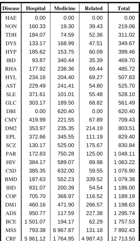
(34) 24 The cost aspects of the Medical Scheme 55-59 data set will also be described. Each line of the Medical Scheme 55-59 data set contains the average Hospital, average Medical and average Related costs associated with a certain unique combination of disease and gender (RETAP, 2007). The term average is used to indicate that each line of unique combination of disease and gender does not. represent a single life, but a multiple number of lives. Only lives treated with a single chronic disease and lives not treated with any chronic disease will be considered. The reason for this is that the Medical Scheme 55-59 data set does not provide a breakdown of the average cost for each chronic disease when the diseases occur simultaneously. For example, lives simultaneously treated for HYP, CMY and DYS might show an average Hospital cost of R1000, but the apportioning of the R1000 among HYP, CMY and DYS will be unknown. The lives with multiple chronic diseases can therefore not be used when average cost differences of the chronic diseases are described. This means that only approximately 89% of lives can be considered, as seen from Table 2.3. Table 2.5 provides information of the average treatment costs associated with female lives. The histograms provided in Figure 2.4 and Figure 2.5 display the breakdown of average costs for female lives. The chronic diseases CRF and MSS have very high average costs. The chronic diseases TDH and HYP have some of the lowest average costs. The female lives not treated for HIV or any chronic diseases, coded as NON, also display very low average costs. Various chronic diseases show a different breakdown of the different types of average costs. The chronic diseases DBI, IBD, SCZ, PAR, CSD and MSS show a higher proportion of average Medicine cost, while TDH, SLE, CMY, IHD, COP, ADS and BCE show a higher proportion of average Hospital cost. Table 2.6 provides information of the average treatment costs associated with male lives. There were no male lives treated for HAE, as seen from Table 2.1. There were also no male lives treated only for DBI. Some male lives were treated for DBI, but these male lives were also simultaneously treated for other chronic diseases. That is why DBI and HAE are not listed in Table 2.6..

(35) Table 2.5:. 25 The breakdown of average cost related to female lives treated for only one chronic. disease and female lives that were not treated for any chronic disease or HIV. That means only 89.64% of female lives are considered. The average cost is apportioned into three categories: Hospital, Medicine and Related.. Disease. Hospital. Medicine. Related. Total. HAE. 0.00. 0.00. 0.00. 0.00. NON. 160.33. 19.30. 39.43. 219.06. TDH. 184.07. 74.59. 52.36. 311.02. DYS. 133.17. 168.99. 47.51. 349.67. HYP. 185.62. 153.75. 60.09. 399.46. IBD. 93.87. 340.44. 35.39. 469.70. RHA. 177.92. 238.36. 69.44. 485.72. HYL. 234.16. 204.40. 69.27. 507.83. AST. 229.49. 241.41. 54.80. 525.70. SLE. 371.61. 101.01. 55.48. 528.10. GLC. 303.17. 189.50. 68.82. 561.49. DBI. 0.00. 620.40. 0.00. 620.40. CMY. 419.99. 221.55. 67.89. 709.43. DM2. 353.97. 235.35. 214.19. 803.51. EPL. 372.66. 345.55. 111.19. 829.40. SCZ. 130.17. 525.00. 175.67. 830.84. PAR. 172.83. 750.28. 125.00. 1 048.11. HIV. 384.17. 589.07. 89.98. 1 063.22. CSD. 385.35. 632.00. 59.55. 1 076.90. BMD. 187.63. 552.23. 339.52. 1 079.38. IHD. 931.07. 200.39. 54.54. 1 186.00. COP. 705.70. 366.97. 116.52. 1 189.19. DM1. 460.16. 471.90. 266.57. 1 198.63. ADS. 950.77. 117.59. 227.38. 1 295.74. BCE. 1 501.07. 194.17. 62.29. 1 757.53. MSS. 793.38. 6 967.87. 131.18. 7 892.43. CRF. 5 961.12. 1 764.95. 4 987.43. 12 713.50.

(36) 26. 800. Female lives. 400 0. 200. Average cost. 600. Related Medicine Hospital. HAE NON TDH DYS HYP. Figure 2.4:. IBD. RHA. HYL AST. SLE GLC. DBI. CMY DM2. The breakdown of average costs related to female lives treated for only one chronic. disease and female lives that were not treated for any chronic disease or HIV.. 12000. Female lives. 8000 6000 0. 2000. 4000. Average cost. 10000. Related Medicine Hospital. EPL. Figure 2.5:. SCZ. PAR. HIV. CSD. BMD. IHD. COP DM1. ADS. BCE MSS. CRF. The breakdown of the average costs related to female lives treated for only one. chronic disease and female lives that were not treated for any chronic disease or HIV. These chronic diseases are associated with relatively high average costs..

(37) Table 2.6:. 27 The breakdown of the average cost related to male lives treated for only one chronic. disease and male lives that were not treated for any chronic disease or HIV. The average cost is split into three categories: Hospital, Medicine and Related.. Disease. Hospital. Medicine. Related. Total. SLE. 0.00. 50.76. 13.82. 64.58. NON. 214.47. 22.02. 34.49. 270.98. TDH. 257.12. 83.42. 72.60. 413.14. ADS. 226.82. 216.74. 14.14. 457.70. HYP. 261.52. 167.19. 62.70. 491.41. HYL. 261.04. 213.25. 48.09. 522.38. IBD. 122.78. 396.76. 28.98. 548.52. BCE. 0.00. 297.64. 267.72. 565.36. BMD. 88.99. 426.97. 62.82. 578.78. AST. 294.14. 241.89. 60.50. 596.53. GLC. 358.53. 205.30. 63.10. 626.93. RHA. 346.44. 233.64. 95.53. 675.61. DYS. 411.20. 202.32. 226.60. 840.12. DM2. 438.06. 237.96. 250.15. 926.17. IHD. 518.39. 255.50. 160.34. 934.23. EPL. 529.41. 350.31. 66.86. 946.58. CSD. 580.28. 488.04. 33.43. 1 101.75. CMY. 712.39. 249.19. 163.20. 1 124.78. HIV. 414.84. 648.40. 71.16. 1 134.40. COP. 698.92. 337.30. 124.63. 1 160.85. SCZ. 785.80. 411.92. 67.33. 1 265.05. PAR. 600.11. 893.81. 55.52. 1 549.44. DM1. 682.35. 521.56. 346.10. 1 550.01. MSS. 0.00. 5 253.77. 76.85. 5 330.62. CRF. 4 374.02. 2 292.40. 5 639.28. 12 305.70.

(38) 28. 800. Male lives. 400 0. 200. Average cost. 600. Related Medicine Hospital. SLE. Figure 2.6:. NON. TDH. ADS. HYP. HYL. IBD. BCE BMD. AST. GLC RHA. DYS. The breakdown of the average costs related to male lives treated for only one chronic. disease and male lives that were not treated for any chronic disease or HIV. These chronic diseases are associated with relatively low average costs.. 12000. Male lives. 8000 6000 0. 2000. 4000. Average cost. 10000. Related Medicine Hospital. DM2. Figure 2.7:. IHD. EPL. CSD CMY. HIV. COP SCZ. PAR. DM1. MSS. CRF. The breakdown of the average costs related to male lives treated for only one chronic. disease and male lives that were not treated for any chronic disease or HIV. These chronic diseases are associated with relatively high average costs..

(39) 29 Figures 2.6 and 2.7 display the breakdown of average costs for male lives. The chronic diseases CRF and MSS have high average costs, which is also the case for female lives. The chronic diseases SLE, TDH and ADS have some of the lowest average costs. Various chronic diseases show a different breakdown of average costs. The chronic diseases SLE, IBD, PAR, BMD and MSS show a higher proportion of average Medicine cost, while TDH, CMY, IHD and COP show a higher proportion of average Hospital cost. The average Related costs tend to be less substantial. Only the chronic diseases CRF, BCE and DYS have a substantial proportion of average Related cost. 2.3. Summary. It is very important to note that the results produced in this chapter only apply to the age band of 55 to 59 years and thus should not be generalised to all age bands of the complete data set. Nonetheless, it was shown that approximately 72% of lives were not treated for any chronic disease and approximately 17% of lives were treated only for one chronic disease. This means that only approximately 11% of the lives were treated for multiple chronic diseases for this age band. It was also shown that the chronic diseases HAE, DBI, ADS, BCE and MSS did not occur often. On the other hand, the chronic diseases AST, TDH, DM2, HYL and HYP occurred more often. Chronic disease rates were used to make a direct comparison between male and female lives, with regard to the occurrence of chronic diseases. It was found that female lives have higher chronic disease rates for DBI, MSS, BCE, SLE, SCZ, BMD, RHA and TDH, while the male lives have higher chronic disease rates for CRF, PAR, HIV, IHD and HYL. Histograms were used to describe the average costs of lives treated for a single chronic disease and lives not treated for any chronic disease. This means that approximately 89% of lives were considered. The reason for this was that average costs could not correctly be allocated between chronic diseases when the chronic diseases co-occur. This is unfortunate because all information regarding average costs of lives treated for multiple chronic diseases had to be discarded, which may limit the relevance of the results. Still, it was found that the chronic diseases CRF, MSS and DM1 were associated with very high average costs for both male and female lives. The male and female lives displayed very low average costs for HYP, HYL and TDH. Lives not treated for any chronic disease or HIV also displayed very low average costs..

(40) 30 It was also found that CMY, IHD, DM2, HYL, DYS, BCE, SLE, ADS and DBI tend to co-occur often with other chronic diseases, while the chronic diseases MSS, PAR, HIV and HAE show much less co-occurrence with other chronic diseases. The usefulness of this information however is limited, as it cannot be used to describe the relationships among the chronic diseases. For example, the histograms showed that the chronic disease CMY co-occurred often with other chronic diseases, but the histograms did not show with which chronic diseases. It will be shown in Chapters 4 and 5 how MDS methods and clustering methods can be used to overcome this limitation of histograms. These methods will show which chronic diseases are more related to one another and which chronic diseases are less related to one another. This can be done by calculating similarities (dissimilarities) between the chronic diseases. Therefore, the question of how to obtain these similarities (dissimilarities) must firstly be addressed. This is done in Chapter 3..

(41) 31. Chapter 3 Calculating Proximities between the Chronic Diseases 3.1. Introduction. There are two measures of proximity in a statistical context, similarity and dissimilarity, which are used to measure how similar and dissimilar objects are to each other. The construction of the similarities (dissimilarities) between the chronic diseases of the Medical Scheme 55-59 data set will be described in this chapter. The similarities (dissimilarities) are based on the number of lives treated for different combinations of chronic diseases. These dissimilarities will be used in Chapters 4 and 5, where the relationships between the chronic diseases will be graphically displayed. The calculation of the dissimilarities is based on various dissimilarity coefficients. Various authors, for example Anderberg (1973), Hubàlek (1982), Gower & Legendre (1986), Cox & Cox (2001) have discussed several dissimilarity coefficients to be used with certain types of variables. However, the discussion in Section 3.2 will focus only on dissimilarity coefficients that are based on binary data, because the chronic diseases are binary variables in the Medical Scheme 55-59 data set. Metric and Euclidean properties of the various dissimilarity coefficients, which are based on binary data, will be discussed in Section 3.3. The metric and Euclidean properties of these dissimilarity coefficients are important to consider when the chronic diseases are graphically displayed in Chapters 4 and 5. It will only be appropriate to use some of these displays if certain metric requirements are met. The R function Dissim.CDL was developed to calculate the dissimilarities between the various chronic diseases. This will be discussed in Section 3.4. Details of the function Dissim.CDL are provided in Appendix A. Various different dissimilarity coefficients will be used to calculate dissimilarities between the chronic diseases. It might not be wrong to consider only one appropriate dissimilarity coefficient, but it might be better to consider various different appropriate dissimilarity coefficients, hoping for robustness against a specific choice (Cox & Cox, 2001, p.12). The techniques that will be discussed in Chapters 4 and 5 take dissimilarities as input, and the results will therefore greatly depend on the choice of dissimilarity coefficient. It is because of this that several dissimilarity coefficients, and not just one, will be used in this study..

(42) 32 3.2. Construction of Similarity and Dissimilarity Coefficients for Binary Data. Let sij represent the similarity coefficient between objects i and j. Most of the similarity coefficients have values in the range [0, 1]. Large values of sij indicate that the two objects are very similar. Dissimilarity coefficients of quantitative data can be obtained directly from the data, but dissimilarity coefficients based on binary, nominal and ordinal data are constructed by transforming the similarity coefficients. Let dij represent the dissimilarity coefficient between objects i and j. A value dij close to zero indicates that the two objects i and j are very similar. Conversely, large values of dij indicate that the two objects are very dissimilar. Dissimilarities often only satisfy the first three of the following axioms of a metric (Kaufman & Rousseeuw, 1990, p. 13): 1. dii = 0 2. dij ≥ 0 3. dij = dji 4. dij ≤ dih+ dhj The fourth axiom does not have to be satisfied in general. However, if it is satisfied then the dissimilarities are actual measures of distance. Table 3.1:. Measure of similarity (dissimilarity) between object r and object s. Object s 1 0 Object r. 1 0. a b c d. p = a+b+c+d. In Table 3.1, a indicates the number of variables out of p that score 1 for both objects r and s, b indicates the number of variables that score 1 for object r and 0 for object s, c indicates the number of variables that score 0 for object r and 1 for object s and d indicates the number of variables that both score 0 for object r and s. Similarity coefficients are usually constructed when the variables are binary. These similarity coefficients are then transformed into dissimilarity coefficients, which are used to construct a dissimilarity matrix. The calculation of the similarity coefficient between objects r and s is based on Table 3.1..

(43) 33 Table 3.2:. Various similarity coefficients for binary data. Similarity coefficient. Formula. Jaccard. srs =. a a+b+c. Dice, Sorensen. srs =. 2a 2a + b + c. srs =. a b+c. Kulczynski 1. if r ≠ s if r = s. =0 Ochiai. srs =. Phi. srs =. Baroni-Urbani, Buser. srs =. a. [(a + b)(a + c)]. 0.5. ad − bc. [ (a + b)(a + c)(d + b)(d + c)]. 0.5. ad + a ad + a + b + c. Kulczynski 2. 1 a a srs = ( + ) 2 a+b a+c. Rao, Russell. srs =. a a+b+c+d. Simple matching coefficient. srs =. a+d a+b+c+d. Yule. srs =. ad − bc ad + bc. Sokal, Sneath, Anderberg. srs =. a a + 2(b + c). Several different similarity coefficients are used in practice. In fact, Hubàlek (1982) gives a very comprehensive list, containing 43 similarity coefficients that are used for binary data. Cox & Cox (2001) and Gower & Legendre (1986) also listed several similarity coefficients. Table 3.2 lists 11 similarity coefficients that are readily used in practice and are based on the suggestions made by Hubàlek (1982). Hubàlek (1982) found that the Jaccard, Dice-Sorensen, Kulczynski 1 and Ochiai similarity coefficients generally work well and that the Phi and Baroni-Urbani-Buser similarity coefficients are reasonable. The results by Hubàlek (1982) are based on an ecological data set and these results are very relevant for the Medical Scheme 55-59 data set, because the ecological data set.

(44) 34 has similar characteristics to the Medical Scheme 55-59 data set. This will be discussed in detail in Section 3.4. The similarity coefficients have to be transformed into dissimilarity coefficients. There are many possible transformations, but Gower & Legendre (1986) suggest the following transformations: dij = 1−sij. (3-1). dij = (1−sij)0.5. (3-2). Kaufman & Rousseeuw (1990) prefer to use the transformation in (3-1), because it tends to lead to a clearer clustering structure. The transformation in (3-2) makes the difference between large similarities more important, but makes it more difficult to obtain small dissimilarities. However, the transformation in (3-2) leads to more dissimilarity coefficients with metric and Euclidean properties. This will be discussed in Section 3.3. 3.3. Metric and Euclidean Properties of Dissimilarity Coefficients for Binary Data. Gower & Legendre (1986) discuss metric and Euclidean properties of many dissimilarity coefficients, for both binary and quantitative data. However, only the Euclidean and metric properties of dissimilarity coefficients based on binary data will be discussed in this section, because the chronic diseases are binary variables in the Medical Scheme 55-59 data set. Let all dissimilarities dij be placed in the dissimilarity matrix D, where [D]ij = dij. Gower & Legendre (1986) define the terms metric and Euclidean in the context of dissimilarity coefficients as follows: Definition 3.1. •. Metric property. D is said to be metric if the metric (triangle) inequality dij+dik ≥ djk holds for all triplets. (i, j, k) and dii=0 for all i.. Definition 3.2. •. Euclidean property. D is said to be Euclidean if n points Pi (i=1,2,...,n) can be embedded in a Euclidean space. such that the Euclidean distance between points Pi and Pj is dij. This implies that dij must be non-negative..

(45) 35 If D is Euclidean, it is also a metric. However, if D is a metric it is not necessarily Euclidean. Gower & Legendre (1986) established various results to determine when dissimilarity coefficients display metric and Euclidean properties. For binary variables, define: Sθ =. a+d a + d + θ (b + c). Tθ =. a a + θ (b + c). where a, b, c and d are defined as in Table 3.1. Most of the similarity coefficients displayed in Table 3.2 can be obtained by using the appropriate choice of θ. Dissimilarities can then be formed by transforming these similarity coefficients by a particular transformation function. The metric and Euclidean properties of these formed dissimilarities will be dependent on which transformation function was used. Gower & Legendre (1986) consider the following two transformations: Dθ = 1 − Sθ Dθ = 1 − Sθ. Dθ = 1 − Tθ Dθ = 1 − Tθ. Gower & Legendre (1986) obtain the following results: The dissimilarity 1−Sθ is metric for θ ≥ 1 and the dissimilarity 1 − Sθ is metric for θ ≥ 1/3. The dissimilarity 1−Sθ may be non-metric for θ < 1 and the dissimilarity 1 − Sθ may be non-metric for θ < 1/3. There are similar results when Sθ is replaced by Tθ. If 1 − Sθ is Euclidean, then so is 1 − Sφ for all φ ≥ θ . A similar result holds when Sθ is replaced by. Tθ. The dissimilarity 1 − Sθ is Euclidean for θ ≥ 1 and the dissimilarity 1 − Tθ is Euclidean for θ ≥ 1/2. However, 1−Sθ and 1−Tθ may be non-Euclidean. Gower & Legendre (1986) use these results to investigate the metric and Euclidean properties of among others the dissimilarity coefficients derived from the similarity coefficients listed in Table 3.2. These results are given in Table 3.3..

(46) 36. Table 3.3:. Metric and Euclidean properties of various dissimilarity coefficients for binary data.. Coefficients. Jaccard Dice, Sorensen Kulczynski 1 Ochiai Phi Baroni-Urbani, Buser Kulczynski 2 Rao, Russell Simple matching coefficient Yule Sokal, Sneath, Anderberg. Dθ = (1−Tθ) Metric Euclidean. Dθ = 1 − Tθ Metric. Euclidean. YES NO. NO NO. YES YES. YES YES. NO NO. NO NO. YES YES. YES YES. NO YES YES NO YES. NO NO NO NO NO. NO YES YES NO YES. NO YES YES NO YES. Note that the Euclidean and metric properties of the Kulczynski 1 and Baroni-Urbani-Buser dissimilarity coefficients are not displayed in Table 3.3. The Kulczynski 1 dissimilarity coefficient can take negative values, so its metric and Euclidean properties are irrelevant (Gower & Legendre, 1986). The Baroni-Urbani-Buser similarity coefficient cannot be written in the form Sθ or Tθ and was not considered by Gower & Legendre (1986). The Euclidean and metric properties of the Baroni-Urbani-Buser dissimilarity coefficient can therefore not be listed. The transformation dij = (1−sij)0.5 may be preferred to the transformation dij = 1−sij, because more of the dissimilarities will have metric or Euclidean properties. However, the choice of transformation will also depend on the problem at hand. Table 3.3 will be used in Chapter 4 where it is important to consider metric and Euclidean properties. 3.4. Calculation of Dissimilarities between the Chronic Diseases. As described in Chapter 2, the Medical Scheme 55-59 data set consists of binary variables where “1” indicates that the lives are treated for the respective disease and where a “0” indicates that the lives are not treated for the disease. It is important to investigate how these chronic diseases are related to one another. Dissimilarities between the chronic diseases need to be constructed and will be based on the number of lives treated for different combinations of chronic diseases. These.

(47) 37 dissimilarities will then be used in Chapters 4 and 5 where the relationships between the chronic diseases will be graphically displayed. A dissimilarity matrix of the objects, and not the variables, of a data set will usually be constructed for most applications. However, in the case of the Medical Scheme 55-59 data set, a dissimilarity matrix of the respective binary variables needs to be constructed, remembering that the chronic diseases are binary variables. This can be done by following the approach of Johnson & Wichern (2002, p.677). The approach uses Table 3.4, which is very similar to Table 3.1, except that the roles of the binary variables and objects are interchanged. The substitution of n (the total number of lives) for p (the number of binary variables) is also required. The similarity coefficients listed in Table 3.2 can then be used in the usual manner to construct the similarities between the chronic diseases. These similarities can then be transformed into dissimilarities. Table 3.4:. Measure of similarity between chronic diseases r and s, where a indicates the. number of lives out of n (total number of lives) that are treated for both chronic diseases r and s, b indicates the number of lives treated for chronic disease r, but not treated for chronic disease s, c indicates the number of lives treated for chronic disease s, but not treated for chronic disease r and d indicates the number of lives that are not treated for chronic diseases r and s. Chronic disease s 1 (YES) 0 (NO) 1 (YES). a. b. 0 (NO). c. d. Chronic disease r. n = a+b+c+d. Hubàlek (1982) shows that it is important to consider whether the binary variables are symmetric or asymmetric, as this will greatly influence the choice of similarity coefficient to be used. Symmetric binary variables are binary variables where code “0” and “1” are equally important. Asymmetric binary variables do not attach equal importance to codes “0” and “1”. The most meaningful outcome is usually coded as “1” and the less meaningful outcome as “0”, where “1” refers to the presence of an attribute and “0” to its absence (Kaufman & Rousseeuw, 1990, p.26). The chronic diseases of the Medical Scheme 55-59 data set should therefore be regarded as asymmetric binary variables, because the presence of a chronic disease is more meaningful than its absence (Kaufman & Rousseeuw, 1990, p.26). It is typical for asymmetric binary variables to have large d values in Table.

(48) 38 3.4, because of more 0-0 matches (Hubàlek, 1982). It was found that the average d value for the Medical Scheme 55-59 data set is 432 times greater than the average a value, which suggests that the chronic diseases are indeed asymmetric binary variables. Various authors suggest omitting d values in the denominator of similarity coefficients when 0-0 matches do not have great importance or if the d values are very large in comparison with the a values (Hubàlek, 1982; Gower, 1985; Sibson et al., 1981; Gower and Legendre, 1986; Kaufman & Rousseeuw, 1990). It can be seen from Table 3.2 that the Simple matching coefficient and the Rao-Russell similarity coefficient include d values in the denominator, and are therefore unlikely to be suitable for application to the Medical Scheme 55-59 data set. So which similarity coefficients should be used? Hubàlek (1982) did a comprehensive study of similarity coefficients based on an ecology data set. The ecology data set is very similar to the Medical Scheme 55-59 data set, in the sense that the ecology data set has large d values and consists of asymmetric binary variables. Hubàlek (1982) compared the different similarity coefficients based on certain criteria and admissibility conditions using the ecology data set. Hubàlek (1982) found that the Jaccard, Dice-Sorensen, Kulczynski 1 and Ochiai similarity coefficients performed satisfactory according to his specified criteria, while the Phi and Baroni-Urbani-Buser similarity coefficients also performed satisfactory, but to a lesser extent than the first-mentioned four similarity coefficients. Various authors also recommend using the Jaccard similarity coefficient when using asymmetric binary variables (Sibson et al., 1981; Kaufman & Rousseeuw, 1990). The R function Dissim.CDL was developed to calculate dissimilarities between all the chronic diseases. Details of Dissim.CDL are provided in Appendix A. The variable Nr.Lives in the Medical Scheme 55-59 data set contains the number of lives that have the same gender and diseases combination. This variable will therefore be used to determine the values of a, b, c and d for all pairs of chronic diseases, as described in Table 3.4. These values are then used to construct the various similarity coefficients sij between all pairs of chronic diseases. The Dissim.CDL function constructs all similarities {sij}, which are then transformed to dissimilarities {dij} by using one of the following transformations: dij = 1−sij or dij = (1−sij)0.5. All dissimilarities {dij} are then placed in a dissimilarity matrix D, where [D]ij = dij. Various dissimilarity matrices will be constructed, where each dissimilarity matrix is based on a different similarity coefficient listed in Table 3.2. These dissimilarity matrices will be used as input structures for the MDS methods and clustering techniques, which will be discussed in Chapters 4 and 5..

No results found