Statistics Preprints Statistics
11-2006
Quick Calculation for Sample Size while
Controlling False Discovery Rate with Application
to Microarray Analysis
Peng Liu
Iowa State University, [email protected]
J.T. Gene Hwang
Cornell University
Follow this and additional works at:http://lib.dr.iastate.edu/stat_las_preprints Part of theStatistics and Probability Commons
This Article is brought to you for free and open access by the Statistics at Iowa State University Digital Repository. It has been accepted for inclusion in Statistics Preprints by an authorized administrator of Iowa State University Digital Repository. For more information, please contact
Recommended Citation
Liu, Peng and Hwang, J.T. Gene, "Quick Calculation for Sample Size while Controlling False Discovery Rate with Application to Microarray Analysis" (2006).Statistics Preprints. 55.
Quick Calculation for Sample Size while Controlling False Discovery Rate
with Application to Microarray Analysis
Abstract
Sample size estimation is important in microarray or proteomic experiments since biologists can typically afford only a few repetitions. In the multiple testing problems involving these experiments, it is more powerful and more reasonable to control false discovery rate (FDR) or positive FDR (pFDR) instead of type I error, e.g., family-wise error rate (FWER) (Storey and Tibshirani, 2003). However, the traditional approach of estimating sample size is no longer applicable to controlling FDR, which has left most practitioners to rely on haphazard guessing. We propose a procedure to calculate sample size while controlling false discovery rate. Two major definitions of the false discovery rate (FDR in Benjamini and Hochberg, 1995, and pFDR in Storey, 2002) vary slightly. Our procedure applies to both definitions. The proposed method is
straightforward to apply and requires minimal computation, as illustrated with two sample t-tests and F-tests. We have also demonstrated by simulation that, with the calculated sample size, the desired level of power is achievable by the q-value procedure (Storey, Taylor and Siegmund, 2004) when gene expressions are either independent or dependent.
Disciplines
Statistics and Probability
Comments
This preprint was published as Peng Liu and J. T. Gene Hwang, "Quick calculation for sample size while controlling false discovery rate with application to microarray analysis",Bioinformatics(2007): 739-746, doi:
Quick Calculation for Sample Size while
Controlling False Discovery Rate with
Application to Microarray Analysis
Peng Liu1 and J. T. Gene Hwang2
1Department of Statistics,
Iowa State University, Ames, IA 50011
2Department of Mathematics and Department of Statistical
Science,
Cornell University, Ithaca, NY 14853
November, 2006
Summary.
Sample size estimation is important in microarray or proteomic experi-ments since biologists can typically afford only a few repetitions. Classical procedures to calculate sample size are based on controlling type I error, e.g., family-wise error rate (FWER). In the context of microarray and other large-scale genomic data, it is more powerful and more reasonable to control false discovery rate (FDR) or positive FDR (pFDR)(Storey and Tibshirani, 2003). However, the traditional approach of estimating sample size is no longer applicable to controlling FDR, which has left most practitioners to rely on haphazard guessing.
We propose a procedure to calculate sample size while controlling false discovery rate. Two major definitions of the false discovery rate (FDR in Benjamini and Hochberg, 1995, and pFDR in Storey, 2002) vary slightly. Our procedure applies to both definitions. The proposed method is straight-forward to apply and requires minimal computation, as illustrated with two sample t-tests and F-tests. We have also demonstrated by simulation that, with the calculated sample size, the desired level of power is achievable by the q-value procedure (Storey, Taylor and Siegmund, 2004) when gene ex-pressions are either independent or dependent.
Key words: Power, Sample Size Calculation, pFDR, Experimental Design,
Genomics
1. Introduction
Microarray and proteomic experiments are becoming popular and important in many biological disciplines, such as neuroscience (Mandel et al., 2003), pharmacogenomics, genetic disease and cancer diagnosis (Heller, 2002). These
Table 1
Outcomes when testing m hypothesis.
Hypothesis Accept Reject Total
Null true U V m0
Alternative true T S m1
Total W R m
experiments are rather costly in terms of both materials (samples, reagents, equipments, etc.) and laboratory manpower. Many microarray experiments employ only a small number of replicates (2 to 8) (Yang and Speed, 2003). In many cases, the sample size is not adequate to achieve reliable statistical inference, resulting in waste of resources. Therefore, scientists often ask the following question. How big should the sample size be?
To answer this question, we will calculate sample size that controls some error rate and achieves a desired power. When calculating sample size for a single test, the error rate to control is traditionally the type I error rate, i.e., the probability of concluding a false positive by rejecting the true null hypoth-esis. However, we are simultaneously testing a huge number of hypotheses, each relating to a gene. Hence, multiple testing is commonly applied in the analysis of microarray data. There are several kinds of error rates to control in this context, such as family-wise error rate (FWER) or false discovery rate (FDR). Assume there arem genes on microarray chips and each gene is tested for the significance of differential expression. The test outcomes are summarized in Table 1, where, for example, V is the number of false posi-tives and R is the number of rejections among the m tests (Benjamini and Hochberg, 1995).
The FWER is defined to be the probability of making at least one false positive error: F W ER =P r(V ≥1). Rejecting each individual test with a type I error rate of α/m guarantees, by Bonferroni’s type of argument, that FWER is controlled at level α in the strong sense, i.e., F W ER≤α for any combinations of null and alternative hypotheses. Benjamini and Hochberg (1995) proposed another type of error to control – FDR, which is defined to be the expected proportion of false positives among the rejected hypotheses:
F DR = E V R|R >0 P r(R >0) . (1)
Storey (2002) proposed to control positive FDR (pFDR), i.e.,
pF DR = E V R|R >0 = F DR P r(R >0) . (2) In many cases of genomic data such as microarray, it was argued in Storey and Tibshirani (2003) that it is more reasonable and more powerful to control FDR or pFDR instead of FWER. However, the sample size has been tradi-tionally calculated with a certain type I error rate and can not be directly applied with FDR control.
Recently, a few papers investigated the needs to calculate sample size while controlling FDR and proposed ways to pursue this goal. Yang et al. (2003) applied several inequalities to get a type I error rate that corresponds to the controlled level of FDR. Due to the inequalities applied, the sam-ple size is likely overestimated. Pawitan et al. (2005) investigated several operating characteristic curves to visualize the relationship between FDR, sensitivity and sample size. Although their approach can be useful in calcu-lating the sample size, no simple direct algorithm was provided. Jung (2005)
derived a formula which relates FDR and the type I error rate. Then FDR is controlled by an appropriate level of type I error rate. Pounds and Cheng (2005) proposed an algorithm to iteratively search for the sample size at which the desired power and controlled level of FDR can be achieved. Since FDR controlling procedure is gaining popularity in multiple testings for many problems including microarray analysis, it is important to be able to calculate sample size needed to control the FDR when designing the experiment.
Here we propose a procedure to calculate the sample size for multiple testing while controlling FDR. First, for any estimate of the proportion of non-differentially expressed genes and the level of FDR to control, we find a rejection region for each sample size. Then power is calculated for the selected rejection region for each sample size. According to the desired power, a sample size is finally decided.
Jung’s approach (2005), which was known to us after we had finished our first draft, is more related to our proposed approach than others. Both Jung’s and our approaches base on the same model assumptions which lead to the same FDR expression. The FDR expression is then controlled by studying its relationship to a quantity, which is the type I error rate for Jung and the critical value (the rejection region) for us. Our approach, however, is more graphical. This allows the visualization of the tradeoff between power and sample size and provides quick answer when the user-defined quantities such as power are modified.
In spite of the similarity, this paper extends the approach further to sev-eral different directions and we find our approach very satisfactory. First, we apply our approach to F-tests which are widely used in microarray data
analysis (Cui et al., 2005). Second, we study our approach carefully for the case when the means and variances for expression levels vary among genes, an important and practical setting for microarray. Third, we also show by sim-ulation, that the q-value procedure for controlling FDR proposed by Storey, Taylor and Siegmund (2004) using our suggested sample size achieves the target power to a satisfactory degree. This answers the question positively as to whether there would be any statistical procedure that can realize the target power claimed by the proposed method. Finally, we also compare our approach with Yang et al. (2003) and Pounds and Cheng (2005) which
provide more well-defined algorithms than other papers. Our simulation
demonstrates that the proposed method is superior.
The paper is organized as follows. Section 2 describes our proposed
method illustrated with two-sample t-tests and F-tests. In Section 3, we report the result of simulation studies that compare the power based on pro-posed method to the actual result from q-value procedure. Section 4 discusses our result.
Codes for the proposed method both in R and in Matlab are available to implement the method. The R code can be applied in conjunction with the
ssize package from bioconductor.
2. Method
In this section, we first illustrate our idea and then show how to apply the proposed method for two designs of microarray experiment.
2.1 Proposed Method
The proposed method is derived from the definition of pFDR. Let H =
In a microarray experiment, H = 1 represents differential expression for a
gene whereas H = 0 represents no differential expression. We assume as
in Theorem 1 of Storey (2002) that all tests are identical, independent and Bernoulli distributed with P r(H = 0) = π0, where π0 is interpreted as the
proportion of non-differentially expressed genes. By Storey’s theorem,
pF DR(Γ) = P r(H = 0|T ∈Γ), (3) whereT denotes the test statistic and Γ denotes the rejection region. Because the number of genes is large, typically ranging from 5,000 to 30,000, the probability of no significant findings is close to zero (Storey and Tibshirani, 2003). Therefore our result also applies to controlling FDR because F DR=
pF DR·P r(R >0). Suppose the level of FDR is chosen to beα, the following relationship is derived via simple algebra (see Appendix A).
α 1−α 1−π0 π0 = P r(T ∈Γ|H = 0) P r(T ∈Γ|H = 1) . (4)
For simplicity in notation, we will denote
Λ = α
1−α
1−π0
π0
. (5)
In order to achieve a FDR level to be α (or less), we choose the rejection region Γ so that the right hand side of Equation (4) is equal to (or less than) Λ (see Appendix A).
2.2 Applications of Proposed Method
Microarray experiments are usually set up to find differentially expressed genes between different treatments. The data of scanned intensity for mi-croarray usually go through quality control, transformation and normaliza-tion, as reviewed in Smyth et al. (2003) and Quackenbush (2002). We assume
that data first go through those steps before statistical tests are applied. Be-fore the experiment, we have no observations to check the distribution. It seems reasonable to make a convenient assumption that the distribution of the pre-processed data is normal and hence two-sample t-tests and F-tests are applicable. The same assumption is also made by other proposed meth-ods to calculate sample size (Dobbin and Simon, 2005; Hu et al., 2005; Hua et al., 2005; Jung, 2005).
2.2.1 Two-Sample Comparison with t-test Suppose we want to find dif-ferentially expressed genes between a treatment and a control group using two-sample t-tests. The tested hypothesis for each gene is H0 : µT,g = µC,g
versus H1 : µT,g 6= µC,g, where µT,g and µC,g are mean expressions of g-th
gene for treatment and control group respectively. Let xgj and ygj denote
the observed gene expression levels for treatment and control group respec-tively for the g-th gene andj-th replicate. Assuming equal variance between treatment and control group, the test statistic for the g-th gene is:
Tg = xg−yg r S2 g 1 n1 + 1 n2 , (6) whereS2 g = 1 n1+n2−2[ Pn1 j=1(xgj−xg)2+ Pn2
j=1(ygj−yg)2] is the pooled sample
variance,xg andyg are the means of observed expression levels for geneg for
the two groups respectively. The test statisticTg has a central t-distribution
under the null hypothesis and noncentralt-distribution under the alternative hypothesis. We reject the null hypothesis if |Tg| > cg, for which cg is to be
determined. Applying Equation (4), we find critical value cthat satisfies: Λ = P r(|Tg|> cg|H = 0) P r(|Tg|> cg|H = 1) = 2·Tn1+n2−2(−cg) 1−Tn1+n2−2(cg|θg) + Tn1+n2−2(−cg|θg) , (7)
where Td(•|θ) is the cumulative distribution function of a non-central t
-distribution withddegrees of freedom and non-centrality parameterθ. More-over, Td(•) is Td(•|θ) for θ = 0. In (7), θg = ∆g σg q 1 n1 + 1 n2 (8)
where ∆g =µT,g−µC,g is the true difference between the mean expressions
of treatment and control groups and σg is the standard deviation for geneg.
In this section, we assume a simplified case that ∆g and σg are identical for
all genes. Section 2.2.3 deals with the more realistic case when ∆g and σg
vary among genes. So the subscript g is dropped in this section.
After we find critical values, power is calculated and sample size will be determined. A special and common case is the balanced design when the two groups have the same sample size, i.e., n=n1 =n2.
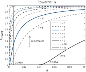
Figure 1 plots the power against Λ for this case. For any selected values of α (FDR level) and π0 (proportion of non-differentially expressed genes),
a sample size can be determined based on this plot for a desired power. As an example, we want to determine the sample size when π0 = 90%. Suppose
a two-fold change is desired (correspondingly, ∆ = log2(2) = 1) and σ =
0.5 from previous knowledge, then ∆
σ = 2. Controlling FDR at 5% results
0 0.02 0.04 0.06 0.08 0.1 0 0.1 0.2 0.3 0.4 0.5 0.6 0.7 0.8 0.9 1 Power vs Λ Λ Power n = 3 n = 5 n = 6 n = 7 n = 8 n = 9 n = 10 n = 15 n=3 n increases n = 5 n = 6 0.0526 0.0058
Figure 1. Summary of relationship between power and Λ = 1−αα π0
1−π0 for
∆
σ = 2. If π0 is estimated to be 90%, controlling FDR at 5% results in
Λ = 0.0058. Along the vertical indicator line, we get power for each sample size. Another indicator line shows the position when Λ = 0.0526 which is a
result of FDR = 5% and π0 = 50%.
the power curves for different sample sizes. A desired power of 80% would determine a sample size of 9. Then 9 samples from each group are needed.
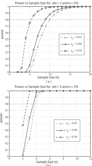
Figures 1 shows a flexible way to apply our method because we can get sample size for any π0 and controlled level ofα. A more straightforward way
to view the result is presented in Figure 2, where we plot power versus sample size when FDR is controlled at 5% and various curves correspond to various
π0’s. For the same example, when π0 = 90% and ∆σ = 2, we determinen = 9
to get at least 80% of power using the middle curve in Figure 2(a).
We shall take σ to be 0.2, which is approximately the 90th percentile of residual standard deviations for the granulosa cell tumor microarray data in Cui et al. (2005). Here 90th percentile is a conservative choice in that if we had used a percentage smaller than 90%, the sample size would be smaller. If still a 2-fold change (∆ = log2(2) = 1) is considered to be true effect
size, then ∆σ = 5. From the middle curve of Figure 2(b), corresponding to
π0 = 0.9, one can determine that a sample size of 4 is needed to obtain at
least 80% of power.
2.2.2 Multi-Sample Comparison withF-test For microarray experiments comparing several treatments, there are different design schemes applied (Yang and Speed, 2003). Suppose without any replication, a design requires
s slides. We call the s slides a set for this design. For example, we want to compare gene expressions among three treatments, such as livers from three genotypes of mice (Horton et al., 2003). If we apply a loop design, as shown in Figure 3, a “set” of three slides is needed for cDNA microarray experiment. Whether the replicates are different biological samples or different technical repetitions, our method is applicable as long as the appropriate parameter (means and variances) are used in the calculation. We recommend to use dif-ferent biological samples in the experiment because this would provide more general conclusions. The question is how many sets of the slides is adequate to obtain a sufficient power and a controlled FDR.
For each individual gene, the experimental design can be formulated with the same linear model for each set i, i= 1,2, ..., n,
Yg,i =Xβg+εg,i , (9)
where βg(p x 1) is the vector of parameters for gene g, Yg,i is the observed
vector for g-th gene in the i-th set, X is the design matrix and εg,i is the
error term. It is assumed that the errors are independent across genes and across sets in this section. For the design in Figure 3, Yg would be the
0 5 10 15 20 0 0.1 0.2 0.3 0.4 0.5 0.6 0.7 0.8 0.9
1 Power vs Sample Size for ∆/σ = 2 and α = 5%
Sample Size (n) π0 = 0.95 π0 = 0.90 π0 = 0.50 power 0 2 4 6 8 10 12 0 0.1 0.2 0.3 0.4 0.5 0.6 0.7 0.8 0.9 1 π0 = 0.95 π0 = 0.90 π0 = 0.50 ( b ) power ( a ) Sample Size (n)
Power vs Sample Size for ∆/σ = 5 and α = 5%
Figure 2. Plot of power versus sample size for t-test. Controlling FDR at 5%, we applied the proposed method to calculate power for each sample size. Panel (a) is for ∆σ = 2 and panel (b) is for ∆σ = 5.
Treatment I - Treatment II Treatment III@ @ @ @ @ I
Figure 3. A design example for microarray experiment to compare gene expressions among three treatments. By convention, each arrow represents one two-color array with the green-labeled sample at the tail and the red-labeled sample at the head of the arrow. This design needs 3 arrays.
parameters can be the gene expression difference between treatment I and II, and difference between treatment I and III (Yang and Speed, 2003). Then the design matrix is
X = 1 0 −1 1 0 −1 .
More complicated models can be constructed for more complex designs and corresponding terms should be added for effects that are not corrected during normalization, such as such array effects, dye effects and block effects. See, for example, Cui et al. (2005). For n sets of slides for a design, the least square estimate of βg is:
ˆ βg = n X i=1 (X0X)−1X0Yg,i/n= (X0X)−1X0 n X i=1 Yg,i/n . (10)
With the assumption of normal distribution for the error, ˆβg is also
nor-mally distributed,
ˆ
βg ∼N(βg, σg2(X 0
X)−1/n) .
We can apply this result and draw statistical inference for these parameters and their linear contrasts.
In general, assume that the question of interest is to test H0 : L0βg = 0
versus H1 : L0βg 6= 0, where L is a p x k coefficient matrix (k ≤ p) or
p x 1 vector for the linear contrast(s) of interest. For simplicity, we omit the subscript g since we assume that the same test is applied for all genes separately. TheF-tests based onnsets can be constructed with the following test statistic: Fn= (L0βˆ)0·[L0(X0X)−1L/n]−1·(L0βˆ)/k Pn i=1(Yi−Xβˆ)0(Yi−Xβˆ)/(d(n)) . (11)
Under H0, Fn follows a F-distribution with k and d(n) degrees of freedom
where d(n) is a function of n and depends on the design. For example, d(n) for the design shown in Figure 3 is 3n −2. Under H1, Fn follows a
non-centralF-distribution with the same degrees of freedom and a non-centrality parameter λ:
λ= (L0β)0Σ−1(L0β) , (12) where Σ =σ2L0(X0X)−1L/n.
Applying Equation (4), we get Λ = P r(Fn> c|H = 0)
P r(Fn> c|H = 1)
= 1−Fk,,d(n)(c) 1−Fk,d(n)(c|λ)
, (13)
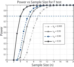
and the same procedure follows to calculate the sample size needed. Here, we choose cto satisfy Equation (13). Using such a c, we calculate the power
P r(Fn > c|H = 1) and then plot the power against n. Figure 4 shows the
resulting curves that are similar as those in Figure 2.
2.2.3 Case for unequal ∆’s and σ’s So far, we have proceeded as if all genes have the same set of parameters. So the average power across all genes would be the same as the power for individual genes. In reality, each gene may have different set of parameters. If we use the two-sample comparison as an example, the gene-specific parameters include σg, the standard deviation,
and ∆g, the true difference between the mean expressions of the treatment
and the control group.
To study the realistic case when ∆g andσg depend on g, we assume that
0 2 4 6 8 10 12 14 16 18 20 0 0.1 0.2 0.3 0.4 0.5 0.6 0.7 0.8 0.9 1
Power vs Sample Size for F test
Sample Size (n) Power π0 = 0.995 π0 = 0.95 π0 = 0.90 π0 = 0.50
Figure 4. For the design as in Figure 3, if we test all treatment means are equal with FDR controlled at 5%, the power of F test is shown for each sample size (number of sets of 3 slides). Here power is calculated when the true difference of log of gene expression levels between treatment I and treatment II to be 1 and difference between treatment I and treatment III to be −0.5,σ = 1.
The distribution can be a parametric or nonparametric one that has been estimated from data of similar experiments. For example, when designing an experiment, a pilot study could be available, based on which the distri-bution of parameters can be estimated. In this case, our procedure can be extended to calculate a sample size while obtaining an average power across all genes. Here by average power, we mean the power integrated with respect to π(∆g, σg),
P r(T ∈Γ|H = 1) =
Z Z
P r(T ∈Γ|H = 1,∆g, σg)π(∆g, σg)d∆gdσg. (14)
we conclude that the FDR is α if Λ = R R P r(T ∈Γ|H = 0) P r(T ∈Γ|H = 1,∆g, σg)π(∆g, σg)d∆gdσg . (15) where Λ = α 1−α 1−π0 π0 .
When we apply this to the t-tests, similar to Equation (7), Equation (15) becomes
Λ = R R P r(|Tg|> c|H = 0)
P r(|Tg|> c|H = 1,∆g, σg)π(∆g, σg)d∆gdσg
, (16)
where the numerator equals 2·Tn1+n2−2(−c) and the denominator equals
1− Z Z Tn1+n2−2(c|θ)π(∆g, σg)d∆gdσg + Z Z Tn1+n2−2(−c|θ)π(∆g, σg)d∆gdσg . (17)
Note that θ is as defined in (8). As before, Td(•|θ) denotes the cumulative
distribution function (cdf) of t-distribution. We then solve for the critical
value c and apply the same procedure to get the sample size needed. The
same technique extends to the F-tests or other tests of interest.
To illustrate our idea in more details, we assume that the mean differ-ence expression level of differentially expressed genes, ∆g, follows a normal
distribution and variances of expression levels for all genes follow an inverse gamma distribution:
∆g ∼ N(µ∆, σ∆2),
σg2 ∼ Inverse Gamma(a, b),
and we use π1(∆g) andπ2(σg) to denote the p.d.f. of ∆g andσg respectively.
FDR and proportion of non-differentially expressed genes (π0). This involves
integrations. To deal with the integration, say in (17), the inner integral equals (see the Appendix B for derivation)
Z Tn1+n2−2 c|∆g σg r 1 n1 + 1 n2 π1(∆g)d∆g =Tn1+n2−2 c r σ2 ∆ σ2 g “ 1 n1+ 1 n2 ”+ 1 |r µ∆ σ2 g 1 n1 + 1 n2 . (18)
For the integration with respect to σg, we can apply adaptive Lobatto
quadrature for numerical integration which allows a stable calculation to get the root of c. The calculation with this numerical integration provides answers instantly. Once we get answers ofcfor each sample size, we calculate power accordingly and find the needed sample size based on power.
3. Simulation
How realistic is the calculated sample size proposed in this paper? More specifically, if the desired power is 80%, FDR = 5% and our approach results in a sample size of 9 for the two-sample comparison with t-test, is there a statistical test that would actually achieve all the operating characteristics with 9 slides? To find out, we simulate data with calculated sample size and perform multiple testing with a FDR controlling procedure. Then we checked:
• whether the multiple testing actually results in desired power for the calculated sample size, and
• whether the observed FDR is comparable with the level that we want to control.
If we can find a statistical procedure that achieves the desired FDR and power at the calculated sample size, our procedure is then demonstrated to be practical. This is indeed the case.
There are several procedures to control FDR, such as the q-value pro-cedure proposed by Storey and Tibshirani (2003) and Storey, Taylor and Siegmund (2004), and the procedures proposed by Benjamini and Hochberg (1995) and Benjamini and Hochberg (2000). These procedures all have the FDR conservatively controlled (Storey et al., 2004). For the purpose of sim-ulation study, we apply the q-value procedure as outlined in Storey et al. (2004) to control FDR. The earlier version of the manuscript applied the procedure in Storey and Tibshirani (2003) and the results were similar to the report here.
We first test the proposed method when observations(genes) are indepen-dent of each other. In a microarray setting, we suppose there are a total of 5000 genes and we have equal sample size for the treatment and the control groups (n1 = n2 = n). Gene specific variances, σg2, are simulated from an
inverse gamma distribution. Same as in Wright and Simon (2003), we chose 1/σ2 ∼Γ(3,1) because this distribution approximates well several microarray data sets that we have been analyzing. For the control group, gene expres-sion values are simulated from N(0, σ2
g). For the treatment group, we set
∆g=0 for non-differentially expressed genes and simulate ∆g from N(2, σ∆2)
for differentially expressed genes, then gene expression values are simulated from N(∆g, σg2).
Table 2
Parameter values in Simulation Study
Parameter Values in Simulation π0 0.995, 0.95, 0.9, 0.8 σ∆ 0.2, 1, 2
ρ 0, 0.2, 0.5, 0.8
There are several parameters involved for the simulation, π0 (the
pro-portion of non-differentially expressed genes), σ∆ (the standard deviation of
effect size) and for the dependent case, the correlation coefficientρ. To evalu-ate the accuracy of our sample size calculation method, we perform the simu-lation with a factorial design and the levels(values) of each factor(parameter) are summarized in Table 2. For each of the 48 parameter settings, the FDR is controlled at 5% for multiple testing.
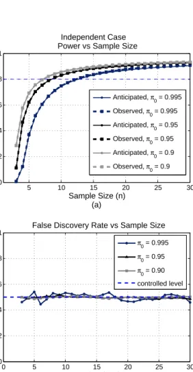
For each parameter setting, we calculate the anticipated power for each sample size and generate the power curve as described in Section 2. We also simulate 200 sets of data and perform t-tests for each data set with q-value procedure (Storey et al., 2004) to control FDR. The observed power is averaged over the 200 simulated data sets and observed proportion of false discoveries is also recorded. Comparing with the simulation results, the an-ticipated power curves based on our calculation are almost indistinguishable from the simulation results for all investigated parameter settings. An exam-ple is shown in Figure 5(a). Hence, our proposed method provides accurate estimate of sample sizes. The observed FDR is also close to the controlled level, 5%, as in Figure 5(b), justifying the validity of the procedure in Storey
et al. (2004).
Since many genes may function as groups, it is very likely that dependen-cies exist in gene expression data. To check the performance of the proposed method when the assumption of independence is violated, gene expression levels are also simulated according to a dependence structure (Ibrahim et al., 2002). Then the same procedure of testing is applied and the resulting power curves are compared with our calculation.
More specifically, gene expression levels for differentially expressed genes are simulated in blocks of 25 according to the following hierarchical structure described in Section 4 of Ibrahim et al. (2002):
µX ∼ N(0, v20) µY ∼ N(2, v20) µXg|µX ∼ N(µX, τ2) µY g|µY ∼ N(µY, τ2) σg2 ∼ Inverse Gamma(3,1) Xgi|µXg ∼ N(µXg, σ2g) Ygi|µY g ∼ N(µY g, σg2).
whereXgiandYgi(g = 1,2, ..., G,i= 1,2, ..., n) are the gene expression levels
for the control group (indexed with X) and treatment group (indexed with
Y) respectively. For non-differentially expressed genes, we simulate µXg the
same as above and set µY g = µXg, based on which we simulate the gene
expression levels Xgi and Ygi. Please note that the correlation coefficient, ρ,
equals v2
0/(v20+τ2) and σ2∆= 2(v20+τ2) with ∆g =µY g−µXg. Examples of
5 10 15 20 25 30 0 0.2 0.4 0.6 0.8 1 Independent Case Power vs Sample Size
Sample Size (n) (a) Power 0 5 10 15 20 25 30 0 0.02 0.04 0.06 0.08 0.1
False Discovery Rate vs Sample Size
Sample Size (n) (b) FDR π0 = 0.995 π0 = 0.95 π0 = 0.90 controlled level Anticipated, π 0 = 0.995 Observed, π 0 = 0.995 Anticipated, π0 = 0.95 Observed, π0 = 0.95 Anticipated, π0 = 0.9 Observed, π 0 = 0.9
Figure 5. Simulation Results. (a) Observed power curves are plotted with dashed lines while the anticipated power curves based on our calculation are plotted with solid lines for different π0’s. For all three π0’s, the differences
between the anticipated and observed power are almost indistinguishable. (b) Observed false discovery rates for the three parameter settings corresponding to (a) are plotted. The controlled level of 5% is indicated with the horizontal dashed line.
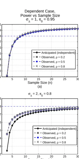
dependent case, 34 of them show results similar as in Figure 6 (a) , which demonstrate that the anticipated power approximates really well of the actual
power. There are two settings that the discrepancy between anticipated
power and calculation is relatively larger than the rest. Figure 6 (b) shows the worse one of the two. Still, the anticipated power based on our calculated sample size is close to the simulation result, and the difference shows that our method will provide a slightly conservative estimate of sample size.
When ∆g and σ2g are the same for all genes, simulation shows that our
method can provide accurate sample size estimation both for independent genes and dependent data similarly as the simulation results shown above.
There are several papers addressing the question of calculating sample size while controlling FDR. Among these papers, Yang et al. (2003) and Pounds and Cheng (2005) provided clearly defined algorithms. We have compared our approach with these methods in the context of 2-sample t-test for fixed ∆g and σ2g. Table 3 shows that, the calculated sample size based
on our proposed approach agrees with the actual sample size needed based on simulation results. Yang’s approach results in similar answers with ours except that in some case, it is a little conservative. Answers from Pounds and Cheng’s algorithm are too liberal in one situation (when ∆/σ=1) and deviate from the right answer a lot more than the other two methods.
4. Discussion
The number of arrays included in microarray experiments directly affects the power of data analysis. It is critical to have a guideline to select a sample size. Because of the huge dimensionality associated with those data sets, controlling FWER is very conservative in many cases (Storey and Tibshirani,
5 10 15 20 25 30 0.1 0.2 0.3 0.4 0.5 0.6 0.7 0.8 0.9 1 Dependent Case, Power vs Sample Size
σ∆ = 1, π 0 = 0.95
Sample Size (n) (a)
Power Anticipated (independent)
Observed, ρ = 0.2 Observed, ρ = 0.5 Observed, ρ = 0.8 5 10 15 20 25 30 0.2 0.3 0.4 0.5 0.6 0.7 0.8 0.9 σ∆ = 2, π 0 = 0.8 Sample Size (n) (b)
Power Anticipated (independent)
Observed, ρ = 0.2
Observed, ρ = 0.5
Observed, ρ = 0.8
Figure 6. Simulation Results. (a) Observed power curves are plotted with dashed lines while the anticipated power curve based on our calculation is plotted with a solid line. The anticipated power based on independence as-sumption approximates well the observed power for all three cases of different correlation coefficients. (a) Observed power curves are plotted with dashed lines while the anticipated power curve based on our calculation is plotted with a solid line. For these cases, the differences between the anticipated and observed power curves are relatively larger and our estimation for such cases is slightly conservative.
Table 3
Comparison of sample size calculation methods including Yang’s approach, Pounds and Cheng’s approach (PC), the proposed method in this paper (LH) with the actual simulation result (Simu). The sample size is selected
based on desired power of 80% and FDR at 5%.
∆/σ=2 Yang’s PC LH Simu π0 = 0.5 8 7 6 6 π0 = 0.9 10 10 9 10 π0 = 0.95 11 11 11 11 ∆/σ=1 Yang’s PC LH Simu π0 = 0.5 22 12 18 18 π0 = 0.9 30 16 29 30 π0 = 0.95 34 18 33 33
2003). Instead, FDR proposed by Benjamini and Hochberg (1995) and Storey (2002) seem to be a more appropriate error rate to control and has been widely applied to microarray analysis. Therefore, it is important to obtain a method to give the sample size that would control the FDR and guarantee a certain power.
The method is straightforward to apply as described in Section 2 for t
and F-tests. The proposed method can be generalized to other tests, as long as there is an explicit form to calculate the type I error and power of an individual test. The method presented in this paper allows calculation for an accurate sample size with minimum effort when designing an experiment.
Acknowledgement
The authors thank Dr. Gregory R. Warnes for insightful comments and suggestions. We also thank Dr. Chong Wang for pointing out the Lobatto Quadrature for numerical integration.
References
Benjamini, Y. and Hochberg, Y. (1995). Controlling the false discovery rate: a practical and powerful approach to multiple testing. Journal of Royal Statistical Society B57, 289–300.
Benjamini, Y. and Hochberg, Y. (2000). On adaptive control of the false discovery rate in multiple testing with independent statistics. Journal of Educational and Behavioral Statistics25, 60–83.
Cui, X., Hwang, J., Qiu, J., Blades, N. J. and Churchill, . A. (2005). Improved statistical tests for differential gene expression by shrinking variance com-ponents estimates. Biostatistics 6, 59–75.
Dobbin, K. and Simon, R. (2005). Sample size determination in microarray experiments for class comparison and prognostic classification. Biostatis-tics 6, 27–38.
Heller, M. J. (2002). DNA microarray technology: devices, systems, and
applications. Annual Review in Biomedical Engineering 4, 129–153. Horton, J. D., Shah, N. A., Park, J. A. W. N. N. A. S. W., m. S. Brown and
Goldstein, J. L. (2003). Combined analysis of oligonucleotide microarray data from transgenic and knockout mice identifies direct srebp target
genes. Proceedings of the National Academy of Sciences 100, 12027–
Hu, J., Zou, F. and Wright, F. A. (2005). Practical FDR-based sample size calculations in microarray experiments. Bioinformatics 21, 3264–3272. Hua, J., Xiong, Z., Lowey, J., Suh, E. and Dougherty, E. R. (2005). Optimal
number of features as a function of sample size for various classification rules. Bioinformatics 21, 1509–1515.
Ibrahim, J. G., Chen, M. and Gray, R. J. (2002). Bayesian models fr gene expression with dna microarray data. Journal of the American Statistical Association 97, 88–99.
Jung, S.-H. (2005). Sample size for fdr-control in microarray data analysis.
Bioinformatics 21, 3097–3104.
Mandel, S., Weinreb, O. and Youdim, M. B. H. (2003). Using cdna microarray to assess parkinson’s disease models and the effects of neuroprotective
drugs. TRENDS in Pharmacological Sciences 24, 184–191.
Pawitan, Y., Michiels, S., Koscielny, S., Gusnanto, A. and Ploner, A. (2005). False discovery rate, sensitivity and sample size for microarray studies.
Bioinformatics 21, 3017–3024.
Pounds, S. and Cheng, C. (2005). Sample size determination for the false discovery rate. Bioinformatics 21, 4263–4271.
Quackenbush, J. (2002). Microarray data normalization and transformation.
Nature Genetics Supplement 32, 496–501.
Smyth, G. K., Yang, Y. H. and Speed, T. (2003). Statistical issues in cdna microarray data analysis. Methods in Molecular Biology 224, 111–136. Storey, J. D. (2002). A direct approach to false discovery rates. Journal of
Royal Statistical Society B64, 479–498.
con-servative point estimation and simultaneous rates: a unified approach.
Journal of Royal Statistical Society B 66, 187–205.
Storey, J. D. and Tibshirani, R. (2003). Statistical significance for
genomewide studies. Proceedings of the National Academy of Sciences
100, 9440–9445.
Wright, G. W. and Simon, R. M. (2003). A random variance model for detection of differential gene expression in small microarray experiments.
Bioinformatics 19, 2448–2455.
Yang, M. C. K., Yang, J. J., McIndoe, R. A. and She, J. X. (2003). Microarray experimental design: power and sample size considerations. Physiological Genomics 16, 24–28.
Yang, Y. H. and Speed, T. (2003). Design and analysis of comparative mi-croarray experiments. Chapman and Hall.
Appendices
Appendix A: Derivation of Equation (4)
Suppose that the test statistic is T and the rejection region is Γ. Let
H = 0 if null hypotheses is true and H = 1 if alternative hypothesis is true. We make the same assumptions as Theorem 1 in Storey (2002), that is, all tests are identical, independent and the probability that the hypothesis is null is P r(H0) = P r(H = 0) =π0. Based on the Bayes rule, the FDR is
P r(H0|T ∈Γ)
= P r(T ∈Γ|H0)·π0
P r(T ∈Γ|H0)·π0+P r(T ∈Γ|H1)·(1−π0)
whereH0 and H1 denoteH = 0 andH = 0 respectively. To control the level
of FDR to be α or less, we set (19) to be less than or equal to α, which is equivalent to: α 1−α 1−π0 π0 ≤ P r(T ∈Γ|H = 0) P r(T ∈Γ|H = 1). (20)
Appendix B: Derivation of Equation (18)
If we let Z stands for a random variable with the standard normal dis-tribution, and let tv(θ) denotes the non-central t distribution with v degrees
of freedom and non-centrality parameterθ, then a random variableX which follows distribution tv(θ) can be viewed as:
X =d Zq+θ
χ2 v v
(21)
where “ = ” denotes that the two random variables have the same distribu-d tion. In the case of two-sample t-test as in Section 2.2.1, for given ∆g and
σg, we know that Tn,g = xg −yg Sg∗ q 1 n1 + 1 n2 ∼tn1+n2−2( ∆g σg q 1 n1 + 1 n2 ) Then Tn,g d = U ,s χ2 n1+n2−2 n1 +n2−2 where U =Z + ∆g σg q 1 n1 + 1 n2
For given σg, we assume that ∆g ∼N(µ∆, σ∆2), then U ∼N µ∆ σg q 1 n1 + 1 n2 , σ 2 ∆ σ2 g 1 n1 + 1 n2 + 1 .
If we scale Tn,g to obtain another non-central t-distribution, we get
Tn,g r σ2 ∆ σ2 g “ 1 n1+ 1 n2 ” + 1 d = r U σ2 ∆ σ2 g “ 1 n1+ 1 n2 ”+ 1 ,s χ2 n1+n2−2 n1+n2−2 d = qZ+p χ2 n1+n2−2 n1+n2−2
where the non-centrality parameter
p = µ∆ σg q 1 n1 + 1 n2 ,v u u t σ2 ∆ σ2 g 1 n1 + 1 n2 + 1 = µ∆ σ2 ∆+σ2g 1 n1 + 1 n2 .
Based on the above result, we can avoid integration with respect to ∆g,
instead, we will have
Z P r(Tn,g < c|∆g)π1(∆g)d∆g =Tn1+n2−2 c r σ2 ∆ σ2 g “ 1 n1+ 1 n2 ” + 1 |p
In the case of n1 =n2 =n, Z P r(Tn,g < c|∆g)π1(∆g)d∆g =T2n−2 c qn·σ2 ∆ 2·σ2 g + 1 µ∆ σ2 ∆+ 2σ2 g n
where Td(•|θ) denote the cumulative distribution function (c.d.f.) of X in