Interpretation, Identification and Reuse of Models. Theory and algorithms with applications in predictive toxicology.

University of Bradford eThesis

This thesis is hosted in

Bradford Scholars

– The University of Bradford Open Access

repository. Visit the repository for full metadata or to contact the repository team

© University of Bradford. This work is licenced for reuse under a

Creative Commons

Licence

.

AND REUSE OF MODELS

THEORY AND ALGORITHMS WITH

APPLICATIONS IN PREDICTIVE TOXICOLOGY

Anna Maria PALCZEWSKA

A thesis submitted for the degree of

Doctor of Philosophy

School of Electrical Engineering and Computer Science

University of Bradford

Keywords: Model interpretation, Model identification, Model governance, Reuse of models, Predictive toxicology, Random forest model, Feature contributions, Pareto optimality

Abstract

This thesis is concerned with developing methodologies that enable exist-ing models to be effectively reused. Results of this thesis are presented in the framework of Quantitative Structural-Activity Relationship (QSAR) models, but their application is much more general. QSAR models re-late chemical structures with their biological, chemical or environmental activity. There are many applications that offer an environment to build and store predictive models. Unfortunately, they do not provide advanced functionalities that allow for efficient model selection and for interpreta-tion of model predicinterpreta-tions for new data. This thesis aims to address these issues and proposes methodologies for dealing with three research prob-lems: model governance (management), model identification (selection), and interpretation of model predictions. The combination of these method-ologies can be employed to build more efficient systems for model reuse in QSAR modelling and other areas.

The first part of this study investigates toxicity data and model formats and reviews some of the existing toxicity systems in the context of model development and reuse. Based on the findings of this review and the prin-ciples of data governance, a novel concept of model governance is defined. Model governance comprises model representation and model governance processes. These processes are designed and presented in the context of model management. As an application, minimum information require-ments and an XML representation for QSAR models are proposed.

new data. It may happen that there is more than one model available for the same endpoint. Which one to chose? The second part of this thesis proposes a theoretical framework and algorithms that enable automated identification of the most reliable model for new data from the collection of existing models. The main idea is based on partitioning of the search space into groups and assigning a single model to each group. The con-struction of this partitioning is difficult because it is a bi-criteria problem. The main contribution in this part is the application of Pareto points for the search space partition. The proposed methodology is applied to three endpoints in chemoinformatics and predictive toxicology.

After having identified a model for the new data, we would like to know how the model obtained its prediction and how trustworthy it is. An inter-pretation of model predictions is straightforward for linear models thanks to the availability of model parameters and their statistical significance. For non linear models this information can be hidden inside the model structure. This thesis proposes an approach for interpretation of a random forest classification model. This approach allows for the determination of the influence (called feature contribution) of each variable on the model prediction for an individual data. In this part, there are three methods pro-posed that allow analysis of feature contributions. Such analysis might lead to the discovery of new patterns that represent a standard behaviour of the model and allow additional assessment of the model reliability for new data. The application of these methods to two standard benchmark datasets from the UCI machine learning repository shows a great potential of this methodology. The algorithm for calculating feature contributions has been implemented and is available as an R package calledrfFC.

This work has been funded by BBSRC and Syngenta (International Re-search Centre at Jealott’s Hill, Bracknell, UK).

The candidate confirms that the work submitted is his own and that appro-priate credit has been given where reference has been made to the work of others.

I would like to thank my husband who has been supportive and under-standing over the years of my PhD studies. I would like to express my gratitude for his advice in research work.

Special thanks go to my supervisors: Prof. Daniel Neagu, Mick Ridley, and Kim Travis for all their support in my professional development, ad-vice and guidance during the entire period of my PhD studies. I would like to thank them for proofreading my thesis.

Dr. Richard Marchese Robinson is thanked for the professional collab-oration, support and advice, and many enjoyable discussions inside and outside of work. I also would like to thank him for testing and debugging the rfFC package.

I would like to thank Dr. Xin Fu for the professional collaboration on data and model governance framework, and implementation of MADFARM prototype.

John Delaney and Dr. Nathan Kidley from the Computational Chemistry Department, Syngenta, are thanked for the professional collaboration, con-sultation and support in chemistry related problems and, finally, for giving me access to the in-house logP dataset.

I would like to thank Prof. Mark Cronin and Dr. Steve Enoch for providing access to the IGC50 forTetraphymenra poriformfismdataset.

Many thanks go to my colleagues Dr. Longzhi Yang and Dr. Paul Trandle with whom I had a pleasure to collaborate during my project.

Finally, I would like to acknowledge the support and funding of Syngenta and BBSRC as part of the Industrial CASE scheme.

Books and Journals

• Anna Palczewska, Jan Palczewski, Richard Marchese Robinson, Daniel Neagu. Interpreting random forest classification models using a feature contribution method. in Integration of Reusable Systems, ser. Advances in Intelligent and Soft Computing, T. Bouabana-Tebibel and S. H. Rubin, Eds. Springer Interna-tional Publishing, 2014, vol. 263, pp. 193–218

• Anna Palczewska, Daniel Neagu, Mick Ridley. Using Pareto points for model

identification in predictive toxicology. Journal of Cheminformatics, vol. 5, no. 1, p. 16, 2013

• Anna Palczewska, Xin Fu, Paul Trundle, Longzhi Yang, Daniel Neagu, Mick Ridley, Kim Travis. Towards model governance in predictive toxicology. In-ternational Journal of Information Management, vol. 33, no. 3, pp. 567–582, 2013

• Xin Fu, Anna Wojak (Palczewska), Daniel Neagu, Mick Ridley, Kim Travis.

Data governance in predictive toxicology: A review. Journal of Cheminformat-ics, vol. 3, no. 1, p. 24, 2011

Conference proceedings

• Anna Palczewska, Jan Palczewski, Richard M. Robinson, Daniel Neagu.

In-terpreting random forest models using a feature contribution method. In Infor-mation Reuse and Integration (IRI), 2013 IEEE 14th International Conference, pp.112–119, 2013.

Kingdom Workshop in Computational Intelligence (UKCI 2011), pp.150–156, 2011

Presentation and posters

• Presentation at Joint Biological Sciences and Product Safety Research

Collab-orations Review Event, Using Pareto Points for QSAR Model Identification in Predictive Toxicology, 2–3 Sep. 2013, Syngenta, Bracknell, UK

• Presentation at IEEE 14th International Conference on Information Reuse and

Integration,Interpreting random forest models using a feature contribution method, 14–16 Aug. 2013, San Francisco, USA

• Presentation at Seminar of Artificial Intelligence Research Group,Using Pareto

Points for QSAR Model Identification in Predictive Toxicology, 11 Jun. 2013, University of Bradford, UK

• Presentation at Seminar of Artificial Intelligence Research Group,Latex for

Sci-entific Writing – A Hands-on Introduction to Latex, 16 Nov. 2012, University of Bradford, UK

• Poster at SEURAT Summer School,A Computer Tool Assisting the Quality

Con-trol of Toxicity Data in Chemical Presentation and Physicochemical Descriptors, 4–8 Jun. 2012, Lisbon, Portugal

• Presentation at Fika Seminar, Searching large graph databases, 3 Feb. 2012,

University of Bradford, UK

• Presentation at Fika Seminar, Single-source shortest path problems: Dijkstra

and A* algorithms, 27 Oct. 2011 University of Bradford, UK

• Poster at The Syngenta Biological Sciences and Product Safety Research Days,

Towards Data and Model Governance in Predictive Toxicology, 19–20 Sep. 2011, Syngenta, Bracknell, UK

Toxicology, 7–9 Sep. 2011, Manchester, UK

• Presentation at Seminar of Artificial Intelligence Research Group,Double

Min-Score (DMS) Algorithm for Automated Model Selection in Predictive Toxicology, 6 Sep. 2011, University of Bradford, UK

Software

Glossary xvii

1 Introduction 1

1.1 Background and Motivation . . . 1

1.2 Problem Description . . . 4

1.2.1 Thesis Aims . . . 5

1.2.2 Methodology and Data . . . 6

1.3 Thesis Structure . . . 7

2 Data and Models in Predictive Toxicology 10 2.1 Predictive Toxicology . . . 10

2.2 Toxicity Data Representation . . . 12

2.2.1 Chemical Information . . . 12

2.2.2 Biological Information . . . 16

2.2.3 Toxic Effect . . . 19

2.3 Data Integration . . . 21

2.4 Models in Predictive Toxicology . . . 23

2.4.1 Quantitative Structure-Activity Relationships . . . 24

2.4.2 Data Preparation . . . 26

2.4.3 Model Development . . . 27

2.4.3.1 Internal Validation . . . 28

2.4.4 External Model Validation . . . 33

2.4.5 Predictive Toxicology Systems . . . 37

2.4.5.1 Ambit . . . 37 2.4.5.2 OCHEM . . . 39 2.4.5.3 JRC QSAR Database . . . 39 2.4.5.4 QSARDB . . . 40 2.4.5.5 OpenTox . . . 41 2.4.5.6 Inkspot . . . 42 2.5 Model Reuse . . . 43 2.6 Summary . . . 46 3 Model Governance 47 3.1 Introduction . . . 47

3.2 Definition of Model Governance . . . 49

3.3 Model Governance Processes . . . 51

3.4 Information Management System for Data and Model Governance . . 53

3.4.1 Policies . . . 54

3.4.2 Implementation . . . 55

3.4.3 Management . . . 56

3.5 Model Governance in Predictive Toxicology . . . 57

3.6 QSAR Model Representation . . . 58

3.6.1 Exchanged Model Representation Formats . . . 58

3.6.2 Minimum Information About a QSAR Model Representation (MIAQMR) . . . 61

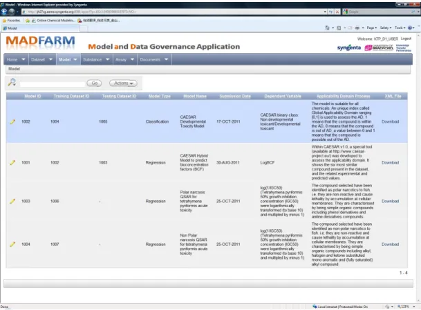
3.7 Model and Data Farm (MADFARM) Prototype . . . 70

3.7.1 MADFARM Design Principles . . . 71

3.7.2 MADFARM Web Interface . . . 72

3.8 Summary . . . 74

4 Model Identification 76 4.1 Introduction . . . 76

4.2 Partitioning Model . . . 78

4.4 Algorithms Based on Pareto Order . . . 81

4.4.1 Pareto Optimality . . . 82

4.4.1.1 Pareto Set . . . 82

4.4.1.2 Pareto Order in Two Dimensions . . . 84

4.4.1.3 Finding a Pareto Set in 2D Vector Space . . . 85

4.4.2 Pareto Algorithms . . . 87

4.4.2.1 Average Pareto Model Identification . . . 91

4.4.2.2 Centroid Pareto Model Identification . . . 92

4.5 Experimental Results . . . 92

4.5.1 IGC50 Prediction forTetrahymena pyriformis . . . 93

4.5.2 LogP Prediction for Syngenta Dataset . . . 101

4.5.3 Prediction of Chemical Persistence in Soil for Syngenta Dataset 107 4.6 Summary . . . 114

5 Model Interpretation 116 5.1 Introduction . . . 116

5.2 Random Forest . . . 118

5.3 Feature Contributions for Binary Classifiers . . . 119

5.3.1 Example of Feature Contributions Calculation . . . 121

5.4 Feature Contributions for General Classifiers . . . 124

5.5 Analysis of Feature Contributions . . . 127

5.5.1 Median Analysis . . . 127

5.5.2 Cluster Analysis . . . 128

5.5.3 Log-likelihood Analysis . . . 130

5.6 Experimental Results . . . 132

5.6.1 Breast Cancer Wisconsin Dataset . . . 133

5.6.2 Cluster Analysis and Log-likelihood . . . 137

5.6.3 Iris Dataset . . . 141

5.6.4 Robustness Analysis . . . 144

5.7 Summary . . . 146

6 Conclusions 147 6.1 Research Contributions . . . 147

6.2 Future Work . . . 152

References 156

2.1 Toxicity data classification. . . 12

2.2 Names and line notations for a tyrosine structure diagram [32]. . . 14

2.3 A fragment of tyrosine - connection table representation [88]. . . 15

2.4 Microarray example of biological data representation [127]. . . 17

2.5 Microarray data processing workflow [47]. . . 18

2.6 Dose-response relationship. . . 20

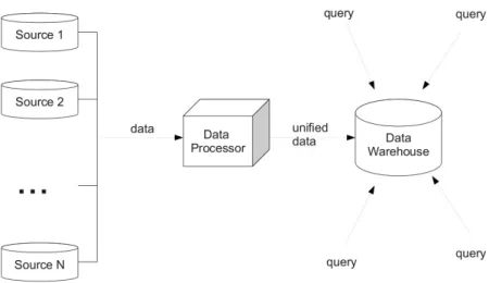
2.7 Simple schema for data integration. . . 22

2.8 QSAR development workflow [113]. . . 26

2.9 Diagnostic test: sensitivity and specificity. . . 30

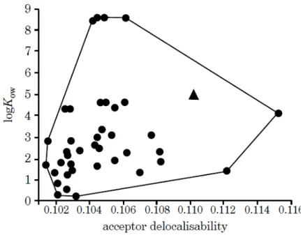
2.10 Example of applicability domain estimation for model predictinglogKow using the acceptor delocalisability descriptor [75]. . . 32

3.1 Decision domains for data governance [62]. . . 48

3.2 Decision domains for model governance. . . 50

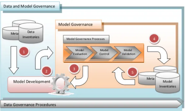
3.3 Model governance processes within a data and model governance frame-work. . . 51

3.4 Information Management System (IMS) for Model Governance. . . . 54

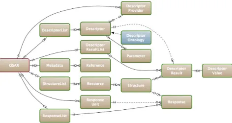
3.5 The QSAR ML structure. . . 60

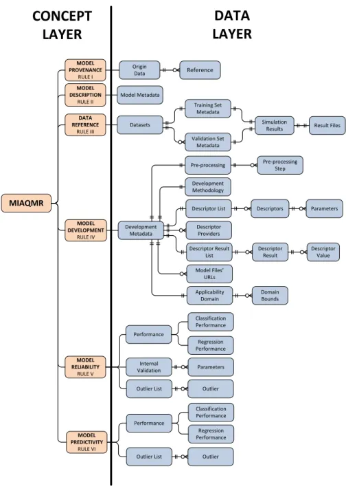
3.6 MIAQMR-ML schema. . . 62

3.7 MADFARM - Browse Assay Interface. . . 72

3.8 MADFARM - Browse Dataset Interface. . . 73

4.1 Search space for Pareto solutions . . . 86

4.2 Collection of models for the IGC50 prediction forTetrahymena pyri-formis. . . 89

4.3 Chemical compounds wrongly associated with the PN model. . . 95

4.4 Chemical compounds wrongly associated with the NPN model. . . 96

4.5 Chemical compounds wrongly associated with the PN model by the oracle model. These chemicals were originally used to train the NPN model. . . 98

4.6 Chemical compounds wrongly associated with the NPN model by the oracle model. These chemicals were used to train the PN model. . . . 99

4.7 Syngenta’s measured LogP dataset. . . 102

4.8 Aggregated minimum absolute error (MAE) and predictive squared co-efficient correlation (Q2) for the 3-APMI 10-cross validation. In each test 1000 chemical were selected. . . 105

4.9 Aggregated minimum absolute error (MAE) and predictive squared co-efficient correlation (Q2) for the 3-APMI 10-cross validation. In each test 2000 chemical were selected. . . 106

4.10 Heatmap of the chemical structure similarity between training and test-ing datasets. . . 109

4.11 Model accuracies vs size of neighbourhood for soil-water models. . . 113

5.1 A Random Forest model for the dataset from Table5.1. . . 122

5.2 The workflow for assessing the reliability of the prediction made by a Random Forest (RF) model. . . 129

5.3 The box-plot for feature contributions within a core cluster for a hypo-thetical Random Forest model. . . 131

5.4 Medians of feature contributions for each class for the BCW Dataset. 134

5.5 The left panel shows permutation based variable importance and the right panel displays Gini importance for a RF binary classification model developed for the BCW Dataset. . . 134

5.6 Comparison of the medians of feature contributions (toward class 1) over all instances of class 1 (black bars) with a) feature contributions for instance number 3 (light-grey bars) b) feature contributions for instances number 194 (grey bars) and 537 (light-grey bars) from the BCW Dataset. The fractions of trees voting for class 0 and 1 for these three instances are collected in Table5.3. . . 136

5.7 Fraction of forest trees voting for the correct class in each cluster for training part of the BCW Dataset. . . 138

5.8 Boxplot of feature contributions (towards class 1) for training instances in each of three clusters obtained for class 1. . . 139

5.9 Log-likelihoods for belonging to the core cluster in class 0 (vertical axis) and class 1 (horizontal axis) for the testing dataset in BCW. Cir-cles correspond to instances of class 0 while triangles denote instances of class 1. . . 140

5.10 Medians of feature contributions for each class for the UCI Iris Dataset. 142

5.11 Log-likelihoods for all instances in UCI Iris Dataset towards core clus-ters for each class. Circles represent the Setosa class, triangles repre-sent Versicolour and diamonds reprerepre-sent the Virginica class. Points corresponding to the same class tend to group together and there are only four instances that are far from their cores. . . 143

5.12 Feature contributions towards class 1 for 100 Random Forest models for the BCW dataset. . . 145

3.1 Model Governance Processes. . . 53

4.1 Analysis of chemical compound similarities in order to highlight the difference of the chemical activity for the TETRATOX dataset . . . . 91

4.2 Comparison of classification algorithms according to a number of cor-rectly classified elements, false positive, false negative and the clas-sifiers accuracies. The polar narcosis model label was defined as the positive class. . . 94

4.3 Model performances and distance comparison of the 3-Pareto neigh-bourhood of the 3-phenyl-1-propanol. . . 96

4.4 Model performances and distance comparison of the 3-Pareto neigh-bourhood of thebenzylamine. . . 97

4.5 Analysis of model prediction accuracies for IGC50 for Tetrahymena pyriformis . . . 97

4.6 Comparison of classification algorithms according to a number of cor-rectly classified elements, false positive, false negative and the clas-sifiers accuracies. The polar narcosis model label was defined as the positive class. . . 100

4.7 Analysis of model prediction accuracies for IGC50 for Tetrahymena pyriformis . . . 101

4.9 Analysis of model prediction accuracies for a LogP estimation for 1000 randomly selected chemicals in 10-CV . . . 104

4.10 Analysis of model prediction accuracies for a LogP estimation for 2000 randomly selected chemicals in 10-CV . . . 106

4.11 Validation of soil-water models. . . 108

4.12 Validation of whole-soil models. . . 108

4.13 Model identification applied to three models for training dataset of soil-water endpoint. . . 111

4.14 Model identification applied to three models for testing dataset of soil-water endpoint. . . 111

4.15 Model identification applied to two models for training dataset of soil-water endpoint. . . 112

4.16 Model identification applied to two models for testing dataset of soil-water endpoint. . . 112

5.1 Selected records from the UCI Iris Dataset. Each record corresponds to a plant. The plants were classified as iris versicolor (class 0) and virginica (class 1). . . 123

5.2 Feature contributions for the Random Forest model from Figure5.1. . 125

5.3 Percentage of trees that vote for each class in RF model for a selection of instances from the BCW Dataset. . . 135

5.4 The structure of clusters for BCW Dataset. For each cluster, the size (the number of training instances) is reported in the left column and the average Euclidean distance from the cluster centre among the training dataset instances belonging to this cluster is displayed in the right col-umn. . . 137

5.5 Feature contributions towards predicted classes for selected instances from the UCI Iris Dataset. . . 142

Greek Symbols Γ Pareto Set

IΓ Initial Pareto Set Other Symbols

q2 _{Predictive Squared Correlation Coefficient}

r2 Squared Correlation Coefficient

Acronyms

AD Applicability Domain

APMI Average Pareto Model Identification BCW Breast Cancer Wisconsin Dataset CAS Chemical Abstract Service

CPMI Centroid Pareto Model Identification CV Cross-Validation

DMS Double Min Score Algorithm

IMS Information Management System InChI IUPAC International Chemical Identifier IT Information Technology

LMO Leave-Many-Out LOO Leave-One-Out MAE Mean Absolute Error

MIAQMR Minimum Information about a QSAR Model Representation NPN Non-Polar Narcosis QSAR Model

OCHEM Online Chemical Modeling Environment

OECD Organisation for Economic Co-operation and Development PMML Predictive Model Markup Language

PN Polar Narcosis QSAR Model QMRF QSAR Model Reporting Format

QSAR Quantitative StructureActivity Relationship

REACH Registration, Evaluation, Authorisation & Restriction of CHemicals RF Random Forest

RMSE Root Mean Square Error

SMILE Simplified Molecular Input Line Entry Specification TPT Tetrahymena pyriformisToxicity

but some are useful...”

Chapter

1

Introduction

This thesis is concerned with methodological problems arising in model identification, interpretation and reuse. Proposed solutions are applied in QSAR modelling frame-work in predictive toxicology.

1.1 Background and Motivation

A phenomenon of fast growing data has been observed in the last decade. Data rep-resentation, integration and storage have turned out to be big challenges and attracted great interest in order to reuse existing information. Garzotto et al. [31] defined the term “reuse” as usage of existing data objects in different contexts and for different purposes. According to the authors, reuse is also a technology that proposes new methods for optimizing data representation, develops strategies and algorithms for ap-plying integration approaches in novel domains, and develops models that can be used for decision-making processes in various application domains.

This thesis focuses on the third aspect of information reuse, that is models. To-gether with the rapidly increasing amount of data, the number and variety of models has increased dramatically thanks to user-friendly machine learning and data mining tools. This has happened especially in domains such as: medicine, life sciences, agri-culture, etc., where models are built based on existing experimental data and are used to make predictions for new data. There is a need to build a framework for efficient model management. This thesis is concerned with developing methodologies that

en-able existing models to be effectively reused. Results of this thesis are presented in the framework of Quantitative Structural-Activity Relationship (QSAR) models, but their application is much more general.

Predictive toxicology is concerned with the development of models that are able to predict the toxicity of chemicals [41]. A large number of publicly available databases, development of computational chemistry and biology, and rapidly increasing number of in-vitro assays have contributed to the development of more accurate predictive models. These models are important for many governmental, academic and business organisations because they enable:

• fast evaluation of chemical toxicity,

• earlier rejection of chemicals that may fail at the chemical development phase,

• reduction in the number of animal tests,

• reduction in the cost of development of new chemical compounds.

The increasing interest in model reuse have also been driven by current requirements of Registration, Evaluation, Authorisation & Restriction of CHemicals (REACH) [94] legislation. This regulatory body accepts chemicals that were tested using inter alia

in silico modelling (predictive models or virtual screening techniques) when models were properly validated and documented. Models must also be statistically significant and robust and have their application boundary defined.

One of the most known and acceptedin-silicomethods, which are used in this the-sis, are Quantitative Structure–Activity Relationship (QSAR) models. They are math-ematical models which relate a biological activity of chemicals to their structural, and physiochemical properties. According to REACH Regulation Annex XI [93], results of QSAR modelling may be used instead of animal testing when: QSAR model was scientifically validated, substance falls within its applicability domain, results are ade-quate for the purpose of classification and labelling and/or risk assessment, and finally, a documentation of the applied method is provided.

The fact that models have become considered as an alternative to animal testing caused a rapid development of in silico methods for screening chemical compounds and a development of model validation techniques in order to prove model reliability

and predictivity. Existing solutions focus on the toxicity data integration and the devel-opment of platforms/systems that provide methods/tools to build high quality models. Gramatica [34] proposed methods for QSAR model validation which have become fun-damentals for the current Organisation for Economic Co-operation and Development (OECD) QSAR validation principles [77]. Tropsha [113] described a workflow for QSAR model development that includes these principles. For example, following the good practice of model development and model validation principles, Hardy et al. [39] introduced interoperable, standard-based framework (OpenTox) for the support of pre-dictive toxicology data management, algorithms, modelling, validation and reporting. Sushko at al. [105] proposed the Online Chemical Modeling Environment (OCHEM) – a web-based platform that aims to automate and simplify typical steps required for QSAR modeling. Both platforms (OpenTox and OCHEM) consist of two major sub-systems: the database of experimental measurements and the modeling frameworks.

The above examples show an interest in QSAR model development, aggregation and utilisation. Whilst the above mentioned platforms provide excellent modelling frameworks and are hosts of models that were generated within such frameworks, model reuse and results validation is left to users. For a collection of models for the same endpoint, a user is required to analyse and compare models with respect to their input variables, applicability domain and accuracy, toidentifythe most suitable one for new data. This is a manual process and requires a lot of effort and knowledge. Model selection can be aided by studying distances between models [49, 73, 111] and their applicability domains [53]. The decision if new data fall inside the applicability do-main is based on the average distance of query data to the data from the applicability domain. For models, where new data fall into their applicability domains, the decision which one should be used is again difficult. For example, there is also no informa-tion about model predictivity in various areas of the applicability domain. This is why there is a need to develop methods that combine: model predictivity and applicability domain in order to provide a framework for automated model identification.

The second element of model reuse is aninterpretationof model predictions for a given data record and each variable used by the model. This interpretation can help to understand how the model makes its prediction and how reliable the prediction is for new data. It might increase the trust in the model. Such interpretation is straightfor-ward for models where there is access to the model variables and parameters. For

non-linear or ”black box“ models such information is hidden within the model structure. The extraction of this information is a challenging problem that has recently begun attracting attention of researchers. For example, see Carlsson et al. [12] who develop a method for local interpretation of Support Vector Machine (SVM) and Random For-est models, and Kiz’min et al. [67] who show how to extract feature contributions in random forest regression models. Interpretation of model prediction is considered par-ticularly valuable in such domains as chemoinformatics, bioinformatics or predictive toxicology [95]. The knowledge of a chemical fragment or chemical properties that contribute to the adverse effect of that chemical compound can support drug design processes.

1.2 Problem Description

The previous section provides examples of toxicity systems that support development of good quality models. Current studies focus on providing user-friendly environments for model building, model validation and reporting. Models are collected in databases for further reuse. Due to an increasing amount of experimental data, we may find more than one model for the same endpoint. In this case a decision which one should be used is not straightforward. The lack of automated methods that allow analysis of models and their selection may discourage potential users. They may prefer to generate a new model, which they will trust, instead of using an existing one. This situation is mostly, but not only, limited to local models that can not become global tools because they were developed for a particular group of chemicals. Such models, even if they can contribute to the fast evaluation of new chemicals, may be forgotten or lost. To address this problem, our main research question is:

How can existing models be efficiently reused?

This thesis aims to answer the above question. The answer comprises three research directions.

The first one, which we callmodel governance, covers the area of model object representation and model management. Developed models must be properly anno-tated and validated prior to their further usage. There should be defined processes that

allow continuous model evaluation (validation and reporting regarding to the organi-zational and authorities requirements). These processes should ensure model quality and security in their future reuse. Model representation should be as much as possible transparent which may allow model exchange initiatives across various organizations.

The second research direction, which we callmodel identification, covers an area of problems related to model selection from a collection of existing models. In cases when there is a number of models for the same endpoint, with overlapping or dis-joint applicability domains, such selection is not trivial. Models must be compared and standard techniques for model selection can not be applied (especially for mod-els with different applicability domains). Incorporating applicability domains in the model comparison can also be difficult because some parameters may not be available. The last research direction,model interpretation, covers the analysis of model pre-dictions. This includes a discovery of mechanisms that lead a model to make a particu-lar decision. This is straightforward for linear models, where there is an easy access to model parameters and their statistical significance. For non-linear and so called ”black-box“ models, this information is hidden inside the model structure and, hence, it is not directly available. Special methods must be designed to enable model interpretation.

1.2.1 Thesis Aims

This thesis addresses the above discussed issues and proposes a theoretical framework and algorithms for each of above presented research directions. This includes defini-tion of the framework for data and model storage, methodology for automated model identification and methods for model interpretation. In respect to each of research directions, this thesis:

1. investigates toxicity data and model formats, and reviews some of the existing toxicity systems in the context of model reuse,

2. defines a new concept of model governance, model governance processes and proposes a theoretical framework for data and model management. This also includes a proposition of a model object representation format,

and applies them to real toxicity data and models for various endpoints to demon-strate their advantage and potential in predictive toxicology,

4. introduces an algorithm for interpreting random forest models which is an ex-tension of feature contributions method of Kuz’min et al. [67] and implements it into an R package,

5. proposes original methods for the analysis of feature contributions and tests them using classification benchmark datasets.

Although this research mostly focuses on the application of novel approaches in predic-tive toxicology, the methodological aspect of this work provides theory and algorithms that can be implemented in any domain that accepts data-driven modelling.

1.2.2 Methodology and Data

This thesis is concerned with methodological problems arising in model reuse. To achieve the research aims, the following existing methodologies were used:

• principles of data governance [20] to inform the design of model governance

processes,

• Pareto optimality approach [23] to solve the bi-criteria problem of model identi-fication. The decision on which model can be the most suitable for new data is a trade-off between the similarity of this data to a group of elements in the search space and the accuracy of the model for these elements,

• the random forest method proposed by Breiman [6] as a basis to develop model

interpretation algorithm,

• the clustering algorithm k-means [40] that is used in analysis of feature

con-tributions.

This research was mainly motivated by the need of model reuse in predictive toxicol-ogy and the solutions were presented in the area for QSAR modelling. In this thesis the following endpoints and models were used:

• IGC50 for Tetrahymena poriformism (TETRATOX data [99]) downloaded from [45], with two QSAR mode of action models (polar narcosis and non polar nar-cosis) reported in the JRC QSAR Model Database [54],

• Measured LogP Syngenta’s in-house dataset, with Syngenta’s in-house model

for CLogP. Two existing tools were also used to calculate LogP: KOWWIN from EPI Suite [28] and MLogP from Dragon software [109],

• Chemical persistence in soil, which was prepared in collaboration with

Syn-genta, and a number of models that were obtained during the competition pub-lished and run by Syngenta at IDEACONNECTION [42],

• Two datasets: Breast Cancer Wisconsin and Iris downloaded from UCI Ma-chine Learning Repository [115,116] and models developed using random forest method.

1.3 Thesis Structure

This thesis is arranged into six chapters and one appendix:

• Chapter 2 – presents a literature review. It includes a review of toxicity data formats, practices in QSAR model development process, a review of current validation techniques and a critical review of some toxicity platforms. Elements of the review presented in this chapter can be found in:

– Anna Palczewska, Xin Fu, Paul Trundle, Longzhi Yang, Daniel Neagu, Mick Ridley, Kim Travis. Towards model governance in predictive toxi-cology. International Journal of Information Management, vol. 33. no. 3, pp. 567–582, 2013

– Xin Fu, Anna Wojak (Palczewska), Daniel Neagu, Mick Ridley, Kim Travis. Data governance in predictive toxicology: A review. Journal of Chemin-formatics, vol. 3, no.1, p. 24, 2011

• Chapter3– introduces a novel concept of model governance. In this chapter, the

are defined: model evaluation, model validation, and model control. A concep-tual framework for data and model governance is established and introduced. To represent a model as an object, six rules were introduced to define mini-mum information about QSAR model representation that are required for model governance. An XML schema based on the proposed rules was defined. The Model and Data Farm (MADFARM) platform was developed in collaboration with Syngenta as a proof of concept of the proposed theoretical framework of model governance. The model governance framework presented in this chapter was published in

– Anna Palczewska, Xin Fu, Paul Trundle, Longzhi Yang, Daniel Neagu, Mick Ridley, Kim Travis. Towards model governance in predictive toxi-cology. International Journal of Information Management, vol. 33. no. 3, pp. 567–582, 2013

• Chapter4– proposes the framework for automated model identification for new

data. This is a theoretical framework that defines a search space (chemical space) and its partitioning model. This model divides a search space into disjoint groups and assigns the most predictive model to each group. To construct such a parti-tion, three approaches were proposed here. One based on the nearest neighbour-hood called the Double Min Score algorithm (DMS) and two based on Pareto optimality which was used to define the Pareto Neighbourhood: Average Pareto Model Identification (APMI) and Centroid Pareto Model Identification (CPMI) algorithms. This is a new approach in model management and mining. This theoretical framework together with proposed algorithms were published in:

– Anna Wojak (Palczewska), Daniel Neagu, Mick Ridley. Double min-score (DMS) algorithm for automated model selection in predictive toxicology.

In United Kingdom Workshop in Computational Intelligence (UKCI 2011), pp.150–156, 2011

– Anna Palczewska, Daniel Neagu, Mick Ridley. Using Pareto points for model identification in predictive toxicology. Journal of Cheminformatics, vol. 5, no.1, p.16, 2013

Tetrahymena pyriformis, LogP for Syngenta dataset, and chemical persistence in soil. Models for prediction of the last endpoint were collected from a compe-tition organised by Syngenta.

• Chapter5– extends to classification problems the feature contribution method,

originally proposed for the interpretation of random forest regression models [67]. Feature contributions explain how a model makes decisions for a given instance. This approach uses a probabilistic interpretation of the random for-est prediction. In this chapter, three novel methods for analysing feature con-tributions: median, clustering and log-likelihood were also introduced. These methods have been tested using general classification benchmark datasets. The results were published in:

– Anna Palczewska, Jan Palczewski, Richard M. Robinson, Daniel Neagu. Interpreting random forest models using a feature contribution method.

In Information Reuse and Integration (IRI), 2013 IEEE 14th International Conference, pp.112–119, 2013.

– Anna Palczewska, Jan Palczewski, Richard Marchese Robinson, Daniel Neagu. Interpreting random forest classification models using a feature contribution method. in Integration of Reusable Systems, ser. Advances in Intelligent and Soft Computing, T. Bouabana-Tebibel and S. H. Rubin, Eds. Springer International Publishing, 2014, vol. 263, pp. 193–218

• Chapter 6– presents conclusions drawn from the work presented in preceding

chapters and offers suggestions for future research.

• Appendix A – includes documentation for the random forest Feature Contri-butions (rfFC) package developed in the project. It implements the method

Chapter

2

Data and Models in Predictive

Toxicology

Reuse of toxicity information facilitates the reduction in the number of animal testing in domains such as: pharmacology, cosmetics or agriculture. This is why data curation and integration have become recent challenges and enjoy a lot of scientific interest. High quality toxicity information is required to build accurate predictive models for toxicity values. This chapter presents various toxicity data representations; data cura-tion and data integracura-tion techniques; a role and process of predicting modelling; and a brief review of existing integrated toxicity platforms. Parts of this review were pub-lished in [30] and [83].

2.1 Predictive Toxicology

Toxicology is defined as the study of adverse effects of chemicals on biological systems such as a cell, tissue, organ or an entire organism [41]. It is the study of symptoms, mechanisms, treatments and detection of chemical toxicity. A large number of in-vivo – in-vitrotests is required in order to explain these toxic effects. The analysis of changes in molecular expression, toxicological parameters, and integrating response data are used to describing functioning organisms [119]. This knowledge is applied in safety evaluation and risk assessment to protect human and environmental health.

po-tential impact of a chemical compound on human or environmental health. Various chemical, biological and toxicological data is combined into sets and used to build predictive models. These models identify parameters that are relevant for a particular toxic effect [41]. When biochemical mechanisms are known, the set of parameters can be pre-defined, reducing the complexity of the model development process. Un-fortunately, biochemical mechanisms are often unknown. In such case, methods for parameter selection should be used to limit the number of suitable parameters that explain a given toxic effect.

Expert systems (often known as rule-driven) and data-driven methods are two main strategies in building predictive models. The expert systems are computer systems that mimic the decision-making ability of a human expert [50]. The most popular rule-based system for the prediction of toxicity (genotoxicity, carcinogenicity or skin sensitization) is DEREK [70]. This system has been developed by LHASA [69] -a not-for-profit comp-any b-ased in Leeds. The rules -are being developed by the ex-pert toxicologists who work for Lhasa or various other exex-perts that use this system. Data-driven methods based on the development of predictive models from experimen-tal toxicity data. There are various methods available (statistical and machine learning methods) and the decision as to which method should be used depends on the ap-plication and complexity of a problem. These methods offer the potential for a fast, rigorous and reliable evaluation of untested chemical toxicity. They are also used in the prioritization of chemical compounds [41] for physical toxicity assays.

A main challenge in predictive toxicology is information reuse. This includes: data integration and model aggregation to provide an interoperable, flexible and transparent framework for automated modelling and testing. The development of good predictive models depends on quality of experimental data [59]. Not complete or not relevant data lead to the generation of inaccurate models. Due to the presence of various tox-icity data representations distributed across many organisations, data integration is a difficult problem. It involves data curation and a data quality assessment to ensure the accuracy of collected information. In literature, one can find ongoing projects aiming to provide integrated platforms for toxicity data exchange across several insti-tutions such as research, business or governmental laboratories. It is an important step to propose standards in toxicity data representation. This will increase the reuse of collected information and facilitate collaboration between various institutions. Model

Figure 2.1: Toxicity data classification.

aggregation has become a valuable technique in toxicity estimation since models have begun to be considered as an alternative for animal testing. The standardisation of the model representation and management policies will lead to an increase in the number of model repositories.

2.2 Toxicity Data Representation

Toxicity data is a combination of chemical, biological and toxicological information (see Figure 2.1). It is used as an input to data-driven approaches to build predictive methods, and to validate these methods by comparing results of predictions with the real measurements. The knowledge of data type and representation leads to a choice of adequate modelling techniques which results in development of fast and efficient predictive methods. In this section, various standards used to represent a chemical compound and biological response are discussed.

2.2.1 Chemical Information

A two-dimensional structural representation of a chemical compound and its semantic nomenclature had been established before the end of the nineteenth century [32]. In the first half of the twentieth century fragment-coding systems were developed to identify sets of sub-structural fragments presented in a molecule. The development of computer

systems and computational chemistry required the presence of more sophisticated and machine-readable representations of a chemical compound.

There are many ways to represent a chemical compound including: names, for-mula, line-symbol notation, molecular representation, physical and chemical proper-ties and fingerprint. Names and indexes like the CAS number are used to identify a query chemical compound and enable fast information (chemical properties) retrieval from large databases. The CAS number is assigned by Chemical Abstract Service [14] to all publicly available chemicals. It does not relate any chemical properties to struc-tures. Its numerical value is assigned in sequential, increasing order when a substance is added into the CAS REGISTRY database. It is a unique numerical identifier with the following format: XXXXXXX-XX-X. The first group may contain up to seven digits, the second group contains only two digits and the last consists of one digit called checksum. This number allow for a quick check if a query chemical compound identifier is correct.

The second group of chemical representations uses their molecular structure. Cur-rently, 1-D, 2-D and 3-D molecular representations are known and there is still a strong interest in deriving new molecular representations [41].

• 1-D representation is a linear string notation of a chemical compound formula (see Figure2.2). The most popular formats are:

– SMILES language (Simplified Molecular Input Line Entry Specification),

– WLN (Wiswesser Line Notation),

– InChI (IUPAC International Chemical Identifier),

– ROSDAL (Representation Of Structure Diagram Arranged Linearly). Over last few years SMILES and InChI have become the most used line nota-tions. SMILES are string notations decoding the molecular structure. They are obtained by printing the symbol nodes encountered in a depth-first tree traversal of a chemical graph [32]. Often, SMILES are not unique. A chemical compound can have a few SMILES notation caused by using different starting points in the traversal procedure. InChI keys describe chemical substances using information layers including: atoms and their bond connectivity, tautomeric information, iso-tope information, stereochemistry, and electronic charge information [74]. In

Figure 2.2: Names and line notations for a tyrosine structure diagram [32].

contrast to widely used CAS registry numbers, SMILES and InChI are com-puted from the structural information and they are readable by experts. They are also are well suited for chemical compound searching and retrieval from large chemical databases.

• 2-D representation includesconnection tables(see Figure2.3). It is a graph rep-resentation G = (V, E)where molecular atoms define a set of graph nodes V

and bonds represent a set of edges E. The connection table consists of three

parts. The first line in the table, called the header block, contains: molecule name and file origin counts of atoms and bonds. The second part, called the atoms block, includes: one line per atom and specifies 2D coordinates, atom symbol, isotope, charge and stereo code. And the last part, called the bonds block, contains: one line per bond (each bond shown once) specifies row num-bers for atoms, and codes for bond type, bond stereochemistry. The molecular graph representation is used for queries in similarity searching and especially in sub-structure searching.

• 3-D representation contains the graph representation extended by 3D

coordi-nates, molecular surface or conformations information. This representation is used in searching pharmacophoric patterns [41].

Figure 2.3: A fragment of tyrosine - connection table representation [88].

Another representation format of a chemical compound is a fragment-based code (index) of its molecule structure. Presence or absence of a certain structural fragment is encoded in a binary vector called a fingerprint[32]. This representation is widely used in substructure searching. There are many similarity metrics such as Hamming distance, Dice coefficient, Euclidean distance to compare two binary vectors to test their similarity. Various measures have been studied by the Sheffield research group in the context of chemical similarity, and the results are presented in [121]. The most common similarity measure between two molecules A and B is Tanimoto coefficient defined as follows:

TAB =

c

a+b₋c (2.1)

whereaandbare numbers of bits set on in the molecules A and B, respectively, andcis

the number of bits set on in both molecules. Comparing with atom-by-atom searching (for a molecular representation), the advantage of using fingerprints is the faster search time for large databases. Unfortunately, the fragment code is not unique. Several struc-tures can have the same fingerprint representation. This is why, thecircular fingerprint

has become very popular. It can be used to generate patterns of various diameter for a molecule. The diameter represents the size of the fragment used to be encoded. By increasing the diameter, one can enrich the information about the molecules. However,

this will also increase the overhead of balancing the fingerprint size and reducing the bit clashes. Nevertheless, fingerprint is a very useful tool to filter a large dataset to find frequently repeated structural patterns.

The last group of chemical representation is called descriptors. There are var-ious physical and chemical properties of a chemical compound calculated from its molecular representation. There are four types of descriptors: topological, geometri-cal, electronic and hybrid. Topological descriptors are derived from connection tables and include information about a number of atoms, bonds and substructures. They includes also topological indices, such as connectivity or kappa indices. From 3D molecular representation, the geometrical descriptors are calculated. They include in-formation such as principal moments of inertia, molecular volume or cross-sectional areas. Electronic descriptors include LUMO and HOMO energies, bond orders or par-tial atomic charges. Various combinations of the above described descriptor types are called hybrid descriptors and they are mostly used in the modelling of quantitative structure-activity relationships. The most comprehensive collection of molecular de-scriptors with detailed review is presented by Todeschini et al. [112]. All descriptors are listed with their definition, symbols and labels, formulas, some numerical exam-ples, data and molecular graphs, while numerous figures and tables aid comprehension of the definitions

2.2.2 Biological Information

Biological information is derived fromin-vitroandin-vivoassays. In-vivodata refers to information collected from experiments or studies done on living organisms. This involves animal testing and clinical trials. The development of molecular biology con-tributed to an increasing number ofin-vitrotests. It is focused on organs, tissues, cells, cellular components, proteins, and biomolecules. In-vitroresearch is more suitable for the deduction of biological changes in the organism (mechanisms of action) and due to its relatively low cost, it is competitive toin-vivostudy [61]. Unfortunately, direct extrapolation fromin-vitrotoin-vivosystems can give misleading results. It is related to the various conditions which are presented during experiments. Successfulin-vitro

tests should usually be followed byin-vivostudies.

Figure 2.4: Microarray example of biological data representation [127].

studies. They are often used to study mechanisms of genotoxicity and carcinogenicity. Various technologies such as cDNA, mRNA microarrays, protein chips and NMR are used in discovery of toxicant pathways and mode of action that may cause a toxic ef-fect [119]. The example of the microarray technique for gene profiling is presented in Figure2.4. DNA chips are used to hybridize two DNA strands. The results are scanned and stored as images. Further, these images are normalised and analysed in order to explain molecular changes.

To provide standards in experiment reporting, the Minimum Information About Microarray Experiment (MIAME) format, was proposed in [5, 25]. It provides a set of rules that contribute to a standardisation of biological experiments. An efficient description of experiments allows for its sufficient interpretation, replication and com-parison with other similar experiments. This process involves: automated data mining techniques and data analysis, standards in experiment descriptions and development of query structures (see Figure2.5).

According to MIAME 2.0 [5], the six following elements must be provided to support microarray publications:

Figure 2.5: Microarray data processing workflow [47].

• experimental design - includes: author, contact information, URL, citations,

ex-periment title, type of exex-periment, exex-perimental variable, quality indicators, re-lationships between the array and sample entities,

• array design - includes: information about array manufacturing given by provider

(platform type, provider, surface type), description of elements or spots used on a surface (e.g. DNA clones), description of specific properties of each element (e.g. DNA sequence),

• samples - include labelled nucleic acids that represent a transcript in a sample for

which the gene expression profile was established (source of the original sample with any biologicalin-vivoorin-vitrotreatments applied, technical extraction of nucleic acids or their subsequent labelling),

• hybridization - includes: laboratory conditions under which the hybridization

were carried out (procedures and parameters),

• measurements - includes: raw data (scans of array), quantification matrices based

on image analysis; specification (gene expression matrix),

• normalization - includes: analysis of multiple samples to identify relative changes

in expression level, different express genes, discovery of gene classes or samples having similar patterns.

2.2.3 Toxic Effect

A chemical substance that causes an adverse effect (toxicant) is recorded together with a dose and its exposure time on a living organism. There are two types of doses: internal and delivered. The first type, often called absorbed dose, describes the total volume of substance that is absorbed and distributed throughout the organism, often expressed in terms of the concentration in plasma/blood or in an organ. The delivered dose is the total dose given to the organism irrespective of what fraction of this is absorbed. This is often expressed in units of mg/kg (amount of chemical/body weight). In short and long term experiments we consider the following types of the exposure times: less then 24 hours, one day up to one month, up to three months and longer than three months. These exposure times are called: acute, subacute, subchronic and chronic exposure, respectively. According to the type of exposure and dose, there are various defined responses of a live organism [52]:

• acute toxicity - an adverse or undesirable effect occurred in a short period of

time (24 hours) that results either from a single or multiple exposures,

• chronic toxicity - an adverse or undesirable effect after long-term exposure (months,

years), usually repeated and lower level exposures,

• local toxicity - an adverse or undesirable effect occurred during contact with toxicant (e.g. skin burns),

• reversible toxicity - an adverse or undesirable effect than can be reversed after the exposure stopped,

• systematic toxicity - an adverse or undesirable effect can be seen in some part of

a live organism resulting from distribution of the chemical around the body,

• delayed/latent toxicity - an adverse or undesirable effect that occurred long after

exposure,

• allergic reaction - reaction to a toxicant caused by an altered state of the normal immune response (never seen for the first exposure but seen with subsequent exposures).

Figure 2.6: Dose-response relationship.

Toxic effects on an organism are related to the amount of exposure often called dose. The dose-response relationships describe the change in the effect caused by different levels of doses after a certain exposure time. Toxicological studies are focused on measurements of dose-responses parameters to define safe and hazardous levels and dosages for various chemicals. The dose-response curve illustrate this relation the X-axis correspond to the concentration of the chemical usually given in milligrams, micrograms, or grams per kilogram of body-weight for oral exposures or milligrams per cubic meter for inhalation exposures. The Y-axis corresponds to the biological response (see Figure2.6). The are many various concentration measures. All of them depend to the exposure time and exposure route (e.g inhalation, dietary). The most common concentration measures are:

• LD50– lethal dose required to kill half the members of a tested population after

a specified test duration,

• EC50 – half maximal effective concentration of a chemicals which induces a

response halfway between the baseline and maximum after a specified exposure time. It is used to measure drug potency,

much of a particular chemical (inhibitor) is needed to inhibit a given biological process by half,

• TD – toxic dose that will produce signs of toxicity in a certain percentage of

organisms,

• NOEL – no-observable-effect-level dose is the highest dose or exposure level of

a chemical that produces no noticeable toxic effect on the organism.

2.3 Data Integration

In-vivoandin-vitrodata are distributed across various resources such as scientific arti-cles, company internal reports, governmental organisation documents and many insti-tutional services. Together with chemical informationin-vitrodata are used to predict

in-vivo toxicity and to prioritise animal testing. Integrating this information in pub-licly available datasets by sufficient extraction, curation and pre-procession is both challenging and extremely valuable.

Data integration is concerned with providing tools for unified access to data from different sources [68]. The data format is defined by the global schema to represent all information which can be query by a user (see Figure 2.7). It is a significant approach for both the enterprise and scientific information integration. Especially, it is also important for the rapid developing life sciences where information exchange is a one of the main challenges to multi-organisation collaboration.

The additional aspect of data integration is to ensure the high quality of combined information that is provided to the user. There are many data quality dimensions such as:

• specification - measures data standards, data models, meta data, and reference

data in terms of existence, completeness, quality, and documentation,

• completeness - measures data attributes according to existence, validity,

struc-ture or content,

• accuracy - measures correctness of database content,

Figure 2.7: Simple schema for data integration.

• timeliness (availability) - measures data validity and availability in a given

frame-work of time,

• security - measures the level of the information security.

Systems which deal with data integration, provide internal rules to ensure data qual-ity and its correctness. Unfortunately, recent studies show lack of consistency in struc-tural representation and systematic chemical identifiers within and between databases [1]. This has an impact for data merging, especially when systematic identifiers are used as a key index for structure integration or cross-querying several databases. This enhances a need for a definition of chemistry standardisation rules and their implemen-tation in order to increase information consistency.

In predictive toxicology the quality of individual data must be assessed according to the correctness of the chemical/biological information and toxicity values. The current standard is to use the Klimisch schema proposed in [63]. This schema provides a set of criteria required to assess data quality:

• reliability – data must be reliable, they must accurately represent the toxic

end-point,

• reproducible – experiment procedures should be independent from the environ-ment and repeated tests in various laboratories should give similar results This schema considers only four categories of data reliability: reliable without re-striction, reliable with rere-striction, not reliable, not assignable. Unfortunately, the Klim-isch schema is very general and it is difficult to distinguish between these categories. To address this gap the reliability assessment tool (ToxRTool) [98] was developed. The transparency of the categories is increased by an extended list of evaluation criteria for scoring toxicity information. Both methods are designed as a set of questions and re-quire a human expert to provide an answer. Thus, the assessment of the data quality is biased by an expert’s experiences and preferences. To reduce this bias and to provide more automated way of quality assessment a fuzzy expert system has been proposed in [126]. This system uses rules from ToxRTool, and is able to evaluate reliabilities of toxicological data based on the currently available metadata.

The process of data integration combined with the information quality assessment is calleddata curation. This process does not stop, the data should be constantly vali-dated, integrated and maintained when there are new experimental results available. It is also an important step in modelling while high quality data is required to build accu-rate predictive models. Poor quality toxicity data with errors and a lack of information contributes to poor predictive performance and low statistical fit. The following sec-tions introduced the processes of model development and their validation in predictive toxicology, as well as discuss the importance of the usage ofin-silicomethods in order to reduce the number of animal tests.

2.4 Models in Predictive Toxicology

Integration of in-vivo and in-vitro data, development of statistical, cheminformatics and bioinformatics algorithms, and data mining tools have led to an enormous increase in the number of models for predictive toxicology. Assessment and application of com-putational methods (often calledin-silico) can be used to reduce animal testing. There are two main contemporary approaches: Quantitative Structure-Activity Relationships (QSAR) which seek to predict the toxicological effects of compounds solely from their molecular structure, and Physiologically Based Pharmacokinetic (PBPK) modelling

which can be used to extrapolate between in-vitro and in-vivo exposure conditions. In subsequent chapters of this thesis all presented work is exclusively concerned with QSAR models.

2.4.1 Quantitative Structure-Activity Relationships

Quantitative structure-activity relationships (QSAR) correlate a chemical structure and properties with biological, chemical or environmental activity [75] whereas SAR asso-ciate the molecular features with its activity [3,41]. Recently, many QSAR modelling tools have been developed using the following techniques: Partial Least Squares Re-gression (PLS) [123], Decision Tree [96], K-Nearest Neighbours (KNN) [60], Support Vector Machine SVM [58], Artificial Neural Network (ANN) [3, 41] and Random Forest [6, 106]. There is also a lot of interest aiming to support automated QSAR modelling [39,46,113] and to build consensus models [128].

QSAR models play the crucial role in virtual screening andin-silico modelling. They are considered to be an alternative to expensive animal testing due to their rela-tively low cost. In the European Union the Registration, Evaluation and Authorisation of Chemicals (REACH) [94] legislation allows for a registration of chemicals which were tested using, inter alia, virtual screening tools. The usage of such modelling tools requires a proof of their reliability and predictivity by a well documented validation process. To make a reliable prediction, a model should be statistically significant and robust, have its application boundaries defined and be validated by an external dataset [33, 114]. Based on this assumption, the first validation principles were assessed in 2002 and then extended in 2004. Currently, they are known as the OECD Principles for QSAR Validation [77]. According to these principles, QSAR models should be associated with the following information:

• Defined Endpoint (Principle 1): The intent of this principle is to ensure clarity in

the endpoint being predicted by a given model, since a given endpoint could be determined by different experimental protocols and under different experimental conditions.

• Unambiguous Algorithm (Principle 2): The intent of this principle is to ensure

from information on chemical structure and/or physiochemical properties. It is recognized that, in the case of commercially-developed models, this information is not always made publicly available. However, without this information, the performance of a model cannot be independently established, which is likely to represent a barrier for regulatory acceptance.

• Defined Domain of Applicability (Principle 3): The need to define an

applicabil-ity domain expresses the fact that QSARs are reductionist models which are in-evitably associated with limitations in terms of the types of chemical structures, physiochemical properties and mechanisms of action for which the models can generate reliable predictions.

• Appropriate Measures of Goodness-of-Fit, Robustness and Predictivity (Princi-ple 4): The wording of the princi(Princi-ple is intended to simplify the overall set of principles, but not to lose the distinction between the internal performance of a model (as represented by goodness-of-fit and robustness) and the predictivity of a model (as determined by external validation).

• Mechanistic Interpretation (Principle 5): It is recognised that it is not always

possible, from a scientific viewpoint, to provide a mechanistic interpretation of a given QSAR, or there even be multiple mechanistic interpretations of a given model. The absence of a mechanistic interpretation for a model does not mean that a model is not potentially useful in the regulatory context. The intention of this principle is not to reject models that have no apparent mechanistic basis, but to ensure that some consideration is given to the possibility of a mechanis-tic association between the descriptors used in a model and the endpoint being predicted, and also to ensure that this association is documented.

In general the QSAR model development process is divided into three steps: data preparation, model generation and validation. These steps together with the above principles require more detailed analysis in the model development process (see Fig-ure2.8). In the following sections, the description of good practices to provide accurate models is presented.

Figure 2.8: QSAR development workflow [113].

2.4.2 Data Preparation

Data quality inherently affects the quality of models [29]. Thus, data curation is a cru-cial step in the data preprocessing phase. This is also a first step in model development process. The processed quality data is further split into two sub-subsets: modelling and external validation sets. There is a big discussion of the best method for the partition percentage. This operation relies on the size of the entire dataset and it is subjectively based on the modeller decision. The best partition should guarantee that these two sub-sets are spread far apart over a wide area of the chemical space and are well balanced [113]. The validation dataset should be distributed across this space to ensure diversity of selected chemicals. Random splitting is the most naive method and unfortunately it does not satisfy the above assumption. There are more efficient partitioning techniques which are based on similarity analysis [34]. The modelling dataset is further split into training and testing datasets. Both these sets are used in model generation and more detailed description is presented in the next section.

Another issue of data preparation is the size of a dataset. The number of chemical compounds included in a dataset should not be either too small or too large. Large

datasets can produce an inefficiency of generated models whereas small datasets may result in inaccurate models. Such inefficiency is related to a selected approach or method processing the large dataset. Each method is limited by an available space and computation time needed to build a model. The dataset should be properly balanced [113, 114]. This means that the number of elements (chemical compounds) from dif-ferent classes or categories (based on their activity) should be equalized. Unbalanced datasets cause higher errors of a correct prediction for the smaller number of elements within a class.

The last step in data preparation is outlier and activity cliff detection [72]. The main hypothesis in QSAR modelling is that similar chemicals have similar properties [51]. Based on this definition, activity cliffs are defined by areas in the chemical descriptors space where the similarity hypothesis does not hold. There are two types of outliers: leverage and activity. They represent either the real values or errors in the structure representation as well as in their activities. There are many methods for outlier de-tection: similarity distance measures, Hotelling’s test, or Cook’s distance [11,75]. In QSAR modelling, the common practice is to remove outliers before model generation. Their presence in the training dataset will lead to model instability. Nerveless, taking outliers into account to develop models and to provide the analysis of their mechanistic interpretation can open a new perspective in building QSAR models.

2.4.3 Model Development

For model generation, the preprocessed modelling dataset is used. This dataset is again partitioned many times using the well known cross-validation (CV) technique. Cross validation involves round estimations of a model. One round of the cross-validation method splits a dataset into training and testing sets. The training dataset is used to generate a model whereas the testing dataset is used to assess its predictivity. Many rounds of CV are applied and validation statistics are collected. A model with the best predictive ability is selected for further external validation tests (see Figure 2.8). The most common CV methods for predictive toxicology are presented in [101,113,114,

123,128] and they involve:

• LMO CV many-out cross-validation) - is generalisation of LOO CV