Characterizing vegetation structure using waveform LiDAR

CHARACTERIZING VEGETATION STRUCTURE USING WAVEFORM LIDAR

BY

KUNXUAN WANG

THESIS

Submitted in partial fulfillment of the requirements

for the degree of Master of Science in Environmental Engineering in Civil Engineering in the Graduate College of the

University of Illinois at Urbana-Champaign, 2016

Urbana, Illinois

Adviser:

A

The structure of light penetration through the canopy plays an important role in water, carbon, and energy fluxes between the biosphere and the atmosphere. Total foliage and foliage distribution are major aspects of canopy structure that significantly influence light and vegetation interaction. Airborne full-waveform LiDAR (Light Detection and Ranging) data contains large amounts of vegetation structural information, and is a powerful tool for providing detailed physical information for large areas of vegetation.

In this thesis, we first provide a complete work flow that extracts and processes waveform LiDAR data for an area of interest. Then we test the feasibility of using waveform LiDAR data to estimate individual tree biomass with limited field samples. We use a voxelization method to generate pseudo-waveforms for individual trees and apply a stepwise regression to find the relationship between pseudo-waveform structural characteristics and biomass estimated by allometric equations using tree survey data. Next, we present a method for describing physical canopy clumping structure for individual trees that provides detailed spatial clumping variations. We utilize the K-means clustering algorithm to extract structure from the large amount of canopy architecture information provided by full-waveform LiDAR. Finally we use representative cluster traits to identify structurally significant clusters. This thesis demonstrates that large amount of canopy structural information can be extracted from waveform LiDAR data. The fine resolution canopy architecture found by methods described in this work can provide valuable information for ecological models.

A

I would like to express my profound gratitude to my advisor Dr. Praveen Kumar for all his support and guidance through out this research. I really appreciate his patience when I am stuck and am grateful for all the insights and ideas along the way.

I would also like to thank to Zhigang Pan from the National Center for Airborne Laser Mapping (NCALM) and Dr. Craig Glennie as well as everyone else at NCALM who helped me start my journey on working with LiDAR data. I could not have started this work with-out them.

Thanks also goes to all the faculty and students who helped in data collection in the summer of 2014, both the airborne remote sensing data as well as the field data.

T

C

L

F

CHAPTER 1 INTRODUCTION . . . 1

1.1 Light and Vegetation Interaction . . . 1

1.2 Light and Biomass . . . 2

1.3 Light and Foliage Clumping . . . 3

1.4 Waveform LiDAR . . . 4 1.5 Thesis Organization . . . 5 1.6 Figures . . . 8 CHAPTER 2 DATA . . . 9 2.1 Data Collection . . . 9 2.2 Data Processing . . . 10 2.3 Figures . . . 15

CHAPTER 3 BIOMASS ESTIMATION . . . 19

3.1 Methods . . . 19

3.2 Results . . . 23

3.3 Figures . . . 26

CHAPTER 4 FOLIAGE CLUMPING . . . 30

4.1 Methods . . . 30

4.2 Results . . . 38

4.3 Figures . . . 42

CHAPTER 5 SUMMARY OF RESULTS . . . 55

5.1 Data Processing . . . 55 5.2 Biomass . . . 56 5.3 Foliage Clumping . . . 57 CHAPTER 6 DISCUSSION . . . 58 CHAPTER 7 CONCLUSION . . . 61 7.1 Summary of Methods . . . 61

7.2 Results and Conclusions . . . 62

L

F

1.1 LiDAR acquisition process and symbolic representation of discrete and

full-waveform LiDAR [Fernandez-Diaz and Carter, 2013]. . . 8

2.1 Summary of relations between raw binary files and the pieces of waveform

data each file contains. . . 15 2.2 Summary of steps in processing waveform LiDAR data. . . 16 2.3 Waveform data extracted for a region where each record in the waveform

is converted into a point. . . 17 2.4 Waveform data of tree displayed as points by giving geolocating each record. 18

3.1 Examples of pseudo-waveforms for individual trees in Allterton Park-1 site. . 26 3.2 Example of relatively well fitted model. Model based on randomly chosen

80% of data. Blue points are data used in the regression. Red points are

the remaining 20% test data. R2 _{value is based on test data only. . . . 27}

3.3 Example of poorly fitted model. Model based on randomly chosen 80% of data. Blue points are data used in the regression. Red points are the

remaining 20% test data. R2 _{value is based on test data only. . . . . 27}

3.4 Biomass results from stepwise regression combined with bootstrapping. All test data are shown in blue. Red circles show the median of all predicted

biomass for each tree. . . 28 3.5 Biomass prediction results using the most prevalent model from 500

boot-strap runs shown in Equation 3.3Resultsequation.3.2.3. . . 29

4.1 Simulated point clouds with 30 cluster centers. . . 42 4.2 K-means cluster evaluation by BIC using a simulated point cloud with 60

clusters. The solid line represents the average of all repeated runs which

are shown as dashed lines. . . 43 4.3 K-means cluster evaluation by minBdist using a simulated point cloud

with 60 clusters. The solid line represents the average of all repeated runs

which are shown as dashed lines. . . 43 4.4 K-means cluster evaluation by Dunn’s index using a simulated point cloud

with 60 clusters. The black line represents the average of all repeated runs,

4.5 K-means cluster evaluation by minimum cluster center distance using a simulated point cloud with 60 clusters. The black line represents the

av-erage of all repeated runs, shown as colored lines. . . 44 4.6 K-means cluster evaluation by a. Dunn’s index and b. minimum cluster

center distance using the waveform LiDAR data of a tree. The black line

represents the average of all repeated runs, shown as colored lines. . . 45 4.7 a. Waveform data of the tree where high intensity shows as green and

low as blue; b,c. Cluster results for K = 130 and K = 220, each color

represents individual clusters. . . 46 4.8 Cluster results forK = 130 andK = 220 colored by cluster intensity. Blue

is less intense, and red the most intense. . . 47 4.9 Cluster results for K = 130 and K = 220 colored by cluster count. Blue

means less records, and red is more records per cluster. . . 48 4.10 Cluster volume forK = 130 andK = 220. Blue represents smaller clusters,

and red represents larger clusters. . . 49 4.11 Cluster diameter results for K = 130 and K = 220. Blue is smaller

diameter, and red is larger diameter. . . 50 4.12 Relationship between cluster diameter and cluster volume. Each point

represents a cluster found by K-means. . . 51 4.13 Comparison of the distribution of different cluster traits: average intensity,

number of records, and cluster diameter. . . 52 4.14 Evaluation of K-means with different number of group (G) using Dunn’s index. 53 4.15 Cluster grouping results by K-means for a. K = 130, and b. K = 220.

CHAPTER 1

INTRODUCTION

1.1

Light and Vegetation Interaction

Vegetation is a major component in all climate studies. It is a major source of evapo-transpiration and respiration. The primary environmental factor that influences vegetation functioning is solar radiation. The amount of light striking the canopy strongly affects pho-tosynthesis, which leads to gas exchanges. Therefore, understanding the interaction between radiation and vegetation is essential in quantifying water, carbon, and energy fluxes between the biosphere and the atmosphere [Kucharik et al., 1999].

There are several important factors that affect light penetration, and therefore its absorp-tion, through the canopy. These include:

ˆ Total foliage. The total amount of foliage can be estimated by leaf area index (LAI), which is one of the most important and thoroughly studies measures of canopy char-acteristics [Bonan, 1993]. It can also be described through vegetation biomass.

ˆ Vertical foliage distribution. The vertical distribution of foliage can be described by leaf area density (LAD), generally presented as a probability density function ranging over the entire height of the canopy. Dutta et al. [submitted] presents a method of estimating tree-wise LAD using the same dataset as that of this thesis.

ˆ Foliage clumping. The non-random distribution of leaves in the canopy leads to clump-ing. Many indices have been developed to describe the severity of foliage clumpclump-ing. However, the majority of these are large scale estimates that assumes uniform amount of clumping through out the canopy.

ˆ Leaf orientation. There are currently no accurate estimations of the orientation of each leaf in the canopy. A mathematical model is generally used as replacement in current models. Random orientation is generally chosen for simplicity.

ˆ Leaf transmittance. The amount of light that can penetrate each leaf in the canopy depends on leaf’s internal structure and chemistry. The LiDAR (Light Detection and Ranging) technology used in this thesis mainly provides structural information, and is unable to quantify this canopy characteristic.

LiDAR data can be used to estimate the total foliage, its distribution and clumping struc-ture. In Dutta et al. [submitted], we used discrete LiDAR data, imaging spectrometer data, and field data to estimate LAD, thus giving us a tree-wise description of vertical leaf distri-bution. Tree-wise LAD provides a relatively fine scale canopy description. However, LAI and vegetation biomass, as an estimation of total vegetation, has traditionally been estimated on the plot level. Foliage clumping, generally described by clumping indices, are also coarse scale measurements.

As current ecological models increase in resolution, these large scale estimates of vegeta-tion characteristics can no longer adequately describe variavegeta-tions in canopy structure. The goal of this thesis is to use waveform LiDAR data to estimate biomass and foliage clumping. Combined with previous works, we hope to provide fine scale estimates of above ground veg-etation biomass, foliage distribution, and foliage clumping in order to inform fine resolution models of vegetation structure.

1.2

Light and Biomass

LAI is one of the most important measurements of total foliage, and it has been widely studied. Our estimation of LAD in Dutta et al. [submitted] can also be used to find the LAI of a tree. Above ground vegetation biomass information is also an important vegeta-tion characteristic used in many ecological models that include terrestrial vegetavegeta-tion in their simulations. Biomass has strong influences on carbon, water, and nutrient cycles. Tradition-ally biomass estimation requires intensive, and often destructive, field measurements. This involves cutting down all sample trees, drying and then weighing each parts of the tree, such as trunk, branches, and leaves, separately [Bombelli et al., 2009]. With the increase in size and sophistication of todays models, acquiring enough biomass data with field sampling as input to such models has become increasingly difficult. Methods exist to estimate biomass from less demanding field measurements. The most common of such methods is using ex-isting allometric equations that are based on the previously mentioned destructive sampling [Ter-Mikaelian and Korzukhin, 1997]. These equations generally require some information

about the trees as input. The most common are diameter at breast height (DBH), i.e., the diameter of the tree measured at 1.3 m from the ground [He et al., 2013], and height of the tree. Measuring DBH and tree height in the field is certainly easier than cutting down and weighting the entire tree. However, with the increase in model range and resolution, acquiring enough data, even the simple measurements needed for allometric equation inputs, might present challenges. One such challenge might be that the areas covered by the model is just too large to traverse easily. Another reason might be that the data is needed on too fine resolution to measure. The most common reason, and also the challenge encountered at our test site, is accessibility. In a dense forest, there are many trees that cannot be measured simply because one cannot reach it due to either terrain, or, as is our case, dense understory. These difficulties impede many models from using rigorous biomass data as input and forces them to use large scale generalized or simulated results. With advances in technology, air-borne LiDAR has the potential to become a convenient tool for acquiring such information on a large scale at fine resolution. The first goal of this thesis is to use LiDAR data to estimate species based tree-wise biomass.

1.3

Light and Foliage Clumping

Clumping of vegetation in forest canopy have important effects on light penetration in the canopy. It affects photosynthesis and many other land-atmosphere interactions such as carbon and water fluxes [Chen et al., 2003, Pisek et al., 2013]. Deriving LAI through optical methods also require knowledge about foliage clumping to obtain the actual LAI [Pisek et al., 2011, 2013]. In this case, foliage clumping accounts for overlaps in foliage that optical methods cannot account for. Due to its importance in a wide range of studies, foliage clumping has been estimated by various methods such as hemispherical photography, sun fleck analysis, and remote sensing [Chen and Black, 1992, Chen et al., 2005, 2003, Pisek et al., 2013, Walter et al., 2003]. Apart from the various methods of obtaining clumping, there are also multiple ways of quantifying it. Currently, the most frequently used description of clumping comes from Chen and Cihlar [1995a,b] and Chen [1996], where the gap fraction and gap size information from hemispherical photos are used along with a ray tracing model to derive a clumping index. Many other indices have been developed, such as that of Pielou [1962], and are used today in conjunction with that of Chen and Cihlar. These indices may vary in the method of derivation, but they all describe the canopy on a fairly large scale. While these traditional clumping indices may be easily ingested by ecological models,

they tend to obscure spatial variations of foliage clump characteristics within the canopy. The second goal of this theis is to provide a physical description of the density and spatial distribution of vegetation using LiDAR derived foliage clump characteristics.

1.4

Waveform LiDAR

With advances in technology, airborne LiDAR has the potential to become a convenient tool for acquiring vegetation structural information on a large scale at fine resolution. Airborne LiDAR is a growing technology where a laser pulse is shot toward the ground from a moving aircraft in a sideways back and forth sweeping motion. When the laser pulse encounters an obstacle, the pulse is scattered back toward the aircraft and the return wave is recorded. The planes location is recorded by a global positioning system (GPS) unit. The plane’s orientation in space is recorded by the inertial measurement unit (IMU) on board [Fernandez-Diaz and Carter, 2013]. By measuring how long it took the laser pulse to return to the plane, the distance from the plane to the obstacle can be calculated. Knowing the angle at which the laser pulse is shot enables us to locate the obstacle relative to the plane. Then, with the plane’s location and orientation in space, we can identify the geolocation of the obstacle. In other words, we know the longitude, latitude and elevation (with respect to any datum) of the obstacle that the laser pulse hit. As the aircraft fly multiple passes over the area of interest, overlapping swaths of land is scanned by thousands of laser pulses per second. This generates a high resolution 3D model of the land surface.

There are two common types of LiDAR data used today, the multiple return discrete LiDAR and the full waveform LiDAR. In this study, we will be using both forms of LiDAR data collected for the same area at the same time. The multiple return discrete LiDAR, or just discrete LiDAR, as shown by the black dots in Figure 1.1, is where a point is recorded each time the outgoing laser pulse hits an obstacle. In a forested area, the first return is generally the top of the canopy, the later returns are likely the understory, and the last return is generally assumed to be the ground. However, under dense canopies, it is possible that neither the understory nor the ground is captured. The reason for the multiple returns is that the laser pulse is not an infinitely thin beam, but spreads out in a narrow cone as it travels through the atmosphere. The size of the beam is called the footprint of the laser pulse. When the cone of light hits the top of the trees, only part of the energy within the footprint is returned, and the rest continues on to generate more returns [Fernandez-Diaz and Carter, 2013]. When the top of the canopy is dense enough to return all energy of the

laser pulse, then only one return is generated. The discrete LiDAR is the most popular LiDAR data used today because it is relatively simple to work with. The discrete LiDAR data generally contains only up to four returns per laser pulse, the first three, and the last return. This limit on the amount of data leads to a compact dataset where each data point contains a lot of information. Therefore, the discrete LiDAR data, or point cloud data, is small and provides a good representation of the Earth’s surface.

The full waveform LiDAR data is derived from the same physical laser return signal as the discrete LiDAR. However, where the discrete LiDAR only records a few points, the full waveform LiDAR digitizes the entire return wave and records the intensity of the return at 1GHz frequency. This translates to one record for about 0.3m travel for the laser. Recording everything at such high resolution generates a much larger dataset compared to the discrete LiDAR. Therefore, the waveform LiDAR data is much harder to work with. However, the full waveform data may be able to resolve finer details not captured in the discrete LiDAR. For instance, discrete LiDAR only captures the first three and the last return. In complex canopy structures, the discrete system will miss everything between the third and last return which the waveform LiDAR will not. Also, when the discrete LiDAR registers a return, there is a set time interval when it will not register another return. This prevents the discrete system from recording an obstacle twice. However it also prevents the discrete LiDAR from observing two closely spaced objects. These situations are resolvable in the waveform LiDAR. In addition, because the shape of each return wave depends on its interactions with the canopy and the ground, waveform LiDAR data can provide the most information for characterizing canopy structure.

Therefore working with LiDAR data presents a trade off. Discrete LiDAR data is easy to work with, but may miss finer details. Waveform LiDAR data is difficult to work with, but captures as much vertical structural information as possible. The key is to use a combination of the two forms of data. Use discrete data when doing larger scale studies, and use waveform data only when finer details are necessary.

1.5

Thesis Organization

Ecological models involving canopy processes have long since started migrating from the simpler big-leaf canopy models to more complex models where processes strongly depend on canopy structure [Chen et al., 2003]. At the same time, models have increasingly higher resolution as computational power grows. These two advancements in ecological modeling

lead to a strong demand for more detailed descriptions of canopy architecture.

In this thesis, we describes our work of using waveform LiDAR data to provide such detailed canopy structural information at fine resolution. Four main factors describe canopy structure as described above, total amount of foliage, foliage distribution, canopy clumping, and leaf orientation. In Dutta et al. [submitted], we estimate tree-wise LAD as a description of foliage distribution. In this thesis, we tackle two other factors that describe canopy structure, total amount of vegetation, and canopy clumping. We estimate total above ground biomass, as a description of total amount of vegetation, using stepwise multiple regression between each tree’s pseudo-waveform characteristics and its biomass derived from field data. The pseudo-waveform is generated by voxelizing all waveform data of the tree. In this thesis, we provide new physical description of canopy clumping structure by applying cluster analysis to the waveform data of each tree. Then we classify the clumps found in waveform data to better understand the connection between clumps in data and actual clumps in the foliage. Unfortunately, airborne LiDAR cannot provide leaf level descriptions.

The thesis is organized as follows:

ˆ Chapter 1 provides background information on the vegetation characteristics currently used in estimating fluxes between land and air, why finer resolution descriptions are needed, and an introduction to airborne LiDAR technology used in this thesis.

ˆ Chapter 2 presents the data used in this thesis as well as the data processing procedure used to prepare raw waveform LiDAR data into usable form.

ˆ Chapter 3 outlines the steps in using LiDAR data for estimating vegetation biomass as well as present the results

ˆ Chapter 4 outlines the steps in using LiDAR data for characterizing foliage clumping and provides the associated results.

ˆ Chapter 5 summarizes results from the two previous chapters.

ˆ Chapter 6 provides discussion about the results as well as issues encountered in the study.

1.6

Figures

Figure 1.1: LiDAR acquisition process and symbolic representation of discrete and full-waveform LiDAR [Fernandez-Diaz and Carter, 2013].

CHAPTER 2

DATA

2.1

Data Collection

The data used in this thesis is collected for sites located in the Upper Sangamon River Basin (USRB) as part of of Critical Zone Observatory for Intensively Managed Landscapes (IMLCZO). USRB is located in east-central Illinois, which has a humid continental climate with hot summers and cold winters. Vegetation mainly consists of row crops, corn and soybean, and some dense mixed forests. The methods in this thesis are mainly targeted toward application in these dense forests.

In the summer of 2014, both remote sensing data and field data were collected around the same time. Airborne remote sensing data includes imaging spectrometer data, also called hyperspectral, and LiDAR data. Lidar data set contains both discrete and waveform data. Flights to obtain the remote sensing data were conducted by the National Center for Airborne Laser Mapping (NCALM). Tree survey data was also collected by students and faculty at the University of Illinois. Only the LiDAR data and field data are used in this study.

2.1.1

LiDAR Data

The LiDAR data was collected using the Optech Gemini Airborne Laser Terrain Mapper (ALTM) on the 4th of August 2014. An infrared laser with wavelength of 1064 nm is used. Nominal flight altitude is 600 m. The scan angle is ±18◦, resulting in a swath width of 367 m. Nominal swath overlap is 185 m. So on average, all areas are scanned twice by the plane to increase point density. With laser pulse repetition frequency (PRF) of 100 kHz and two passes, the resulting discrete point cloud has a density of 7.8 points/m2. Beam divergence is 0.8 mrad, which results in a 0.24 m radius footprint at ground level. Compared to others, this LiDAR system can be considered a small footprint LiDAR with medium to high density.

The discrete LiDAR data was processed by NCALM and is divided into 1 km square tiles. The waveform data was not processed and remains as separate binary files.

2.1.2

Field Data

Tree survey data was collected from July 31st to August 4th 2014 in order to coincide with the airborne remote sensing data collection. Four sites within the USBR were sampled Allerton Park-1, Allerton Park-2, Home Forest Site, and Lake of the Woods. These four sites are located along the riparian forest corridor of the Sangamon River and are mainly dense mixed forests as previously mentioned.

For each site, tree characteristics data collected included stem location, species, crown width, tree height, height of the bottom of the crown, and diameter at breast height (DBH). Various tools used include tape measures, field GPS, total station, and clinometer. Plot level LAI was measured using LAI-2200C plant canopy analyzer. Tree species were identified by comparing leaf samples with published species identification guides [Mohlenbrock, 1973].

2.2

Data Processing

Out of the three datasets used in this thesis, tree survey data (in csv form) and discrete LiDAR data (as tiled point clouds) can be ingested relatively easily. However, our goal is to use waveform LiDAR data to quantify details that may not be captured in the discrete LiDAR data. The discrete LiDAR data was processed by NCALM after they collected the data, but the waveform data was not. They are given as a set of raw binary files. Figure 2.1 shows a summary of the important waveform data in each file and their relations to each other. We must first process the waveform data into usable form for our study. One challenge of working with waveform LiDAR data is the limited software support. So the waveform LiDAR data used in our study are completely processed by original code using Python starting with raw binary files using an object oriented approach. The processing steps are detailed below. A schematic summarizing processing steps is shown in Figure 2.2.

2.2.1

Read Files

The raw waveform LiDAR data is recorded in three separate binary file with different formats DF2, IX2, and CSD. In Figure 2.1, files are enclosed in rectangles, and data are enclosed in ellipses. To construct each waveform, pieces of data must be extracted from all three files. The DF2 file, shown as light red in Figure 2.1, contains the actual digitized intensities of the outgoing and return signals as well as time interval information between when the laser pulse left the digitizer and when it returned. The time interval is the number of cycles of the digitizer’s processor. A PCount factor is needed to convert the time interval information in the DF2 file to seconds. This factor is found in the IX2 file, shown as dark red in Figure 2.1, which is an indexing file that corresponds to the DF2 file. Together, the time interval information and the PCount factor gives the exact linear distance between the start of the outgoing signal (assumed to be the plane location) and that of the return signal.

To fully geolocate the waveform, plane location and orientation as well as scan angle of the laser are needed. These location information is recorded in the CSD file, labeled CSD Record in Figure 2.1, as each laser fires, and each record contains an associated GPS time. The IX2 file can also be used to retrieve GPS time for each waveform. Waveforms can then be matched to its corresponding location information using the two GPS times. To retrieve waveform GPS time from the IX2 file, the following equation is used:

T(Wf,r) =Tf +r(

Tf+1−Tf

Rf

) (2.1)

Where T refers to GPS time, and Wf,r is the rth waveform in frame number f. Tf and Tf+1

refers to GPS time of frame f and that of the subsequent frame. Rf is the total number of waveform in frame f. Here a frame is just an organizational unit used in the IX2 file can contains around 13000 waveforms. Since the IX2 file only contains GPS time record for the start of each frame, interpolation is used to assign GPS time location to each waveform. This process of combining pieces of information from all raw binary files is labeled as Read from files in Figure 2.2. The result is a Python object that we defined called Wave. It contains all intensity records of a single wave as well as geolocation information.

2.2.2

Process Waveform

After all information for one waveform is collected, we then geolocate the wave by assigning location to each digitized intensity record in the waveform. To do this, the range Di, linear

distance of intensity recordiin the return wave from the plane, is calculated. Then rotational matrices are used to apply scan angle and plane orientation to the range. Calculations are shown in the following equation:

   X Y Z    Wi =    X Y Z    pl +RRP Y   Rx(a)    0 0 Di   −    lx ly lz       (2.2)

In a simpler representation, equation 2.2 can be written as follows:

LWi =Lpl+R

RP Y _(R

x(a)Di−e) (2.3)

Where RRP Y _{= R}

z(Y)Ry(P)Rx(R). Rx(a) represents a 3D rotation matrix that applies rotation of angle a around the x-axis to some vector in Euclidean space. Similarly, Ry(P) means rotation of angleP around the y-axis. a is the scan angle of the laser, R, P, Y are the

roll, pitch, yaw angles of the plane.

LW is the location of one digitized record in the waveform. Lpl is the location of the plane.

Di is the vector representation of Di, and e is an error term that account for misalignment and IMU offset. Error values can be found in the header of the CSD file labeled as CSD Headerin Figure 2.1.

Once the wave is geolocated, baseline intensity registered by the sensor is removed from the wave by subtracting a constant representative value to maintain comparability between waveforms. This step of geolocating and processing individual waveforms is labeled asProcess Wavein Figure 2.2.

2.2.3

Correct Errors

At this point, the geolocation of each wave is not exactly correct. Empirical offsets in the data exists due to offset in sensors and datum conversion. The resulting waveform data must be compares to the discrete LiDAR data produced by NCALM using commercial software for corrections. These offsets include offset in range, heading, as well as an offset in GPS time used to match waveform data to plane location and orientation. In order to compare the waveform to the discrete point cloud data, the record with the max intensity in each wave is extracted and combined into a set of point cloud data.

Range offset can be found automatically by comparing corresponding data points in each dataset. Heading offset can be found by comparing the angle of one scan line of data.

However, GPS time offset must be corrected by guess and check. A GPS time offset results in one waveform using the geolocation of an earlier (or later) waveform. This error is most noticeable between two adjacent scan lines in sloped surfaces such as angled roofs. If the offset exists, then the two adjacent scan lines of the same roof will display a horizontal offset. So the offset must be corrected by adding a constant to the GPS time of each waveform. Different constants are tried and checked visually until adjacent scan lines in roofs match. This process of finding offsets in the waveform data is labeled asCorrect Errorsin Figure 2.2. Once offset values are found, either by automatic or visual comparison, we must restart the process at the beginning by reading from raw data and geolocate waveforms while including the calculated offsets.

2.2.4

Extract Waveforms

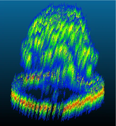
The previous sections describe how data is extracted from raw binary files and combined into a list of waveforms (Wave List). However, waveform LiDAR data is large and difficult to work with, and generally data for the entire site is not needed. Therefore, we develop an algorithm to extract a section of interest in the waveform data based on discrete LiDAR point clouds. Using the point cloud of an area of interest, we find all GPS time intervals the data spans. These intervals will not be continuous in time as the point cloud can contain data from multiple flight lines and the laser can pass in and out of the area of interest as it scan along the flight line. By applying the processes described in previous sections to only waveforms with in the GPS time intervals, we can extract needed waveform information with minimum computation. Figure 2.3 shows the Allerton Park-1 site, and 2.4 shows the sample tree used to test the foliage cluster analysis method described in Chapter 4. In order to display the waveform data for an extracted region, all records in each waveform is converted into a geolocated point and shown as a point cloud by the free CloudCompare software.

2.2.5

Process Wave List

Once a Wave List extracted for a region of interest, further processing might be needed to prepare waveform data for our models. This step is labeled as Process Wave List in Figure 2.2. However, different procedures are required for different models. Therefore, this step will be described in the following Chapter along with studies that use the data produced by the procedures described in this Chapter.

2.3

Figures

Figure 2.1: Summary of relations between raw binary files and the pieces of waveform data each file contains.

Figure 2.2: Summary of steps in pro cessing w a v eform LiD A R data.

Figure 2.3: W a v eform data extracted for a region where eac h record in the w a v eform is con v erted in to a p oin t.

CHAPTER 3

BIOMASS ESTIMATION

In this chapter, we describe how we used waveform data extracted for individual trees along with field data in an attempt to estimate above ground biomass for each tree. Traditional methods for calculating biomass involves destructive sampling of trees. More recent methods such as using allometric equations also require some field measurements such as DBH and tree height.

Using airborne LiDAR data may be the only way to find fine scale biomass data for large areas. LiDAR data gives a detailed description of tree size and structure, with directly influences biomass. So in this chapter, we attempt to relate a tree’s waveform characteristics to it biomass calculated from field data.

First we describe the methods used in the analysis, then we present our results. Conclu-sions will be presented in Chapter 6 and 7.

3.1

Methods

In this section, we first describe how we extract waveform characteristics for individual trees, then we present our regression analysis that tries to relate the waveform characteristics of each tree to biomass information derived from field data.

3.1.1

Process Wave List

To find individual trees, the canopy height model is used as input to Envi-Lidar. This program assumes circular tree crowns and delineates individual trees with location and radius as output. Next, using the delineated point cloud information as input to the data processing procedure described in Chapter 2, the list of waveforms, or Wave List, for each tree can be extracted.

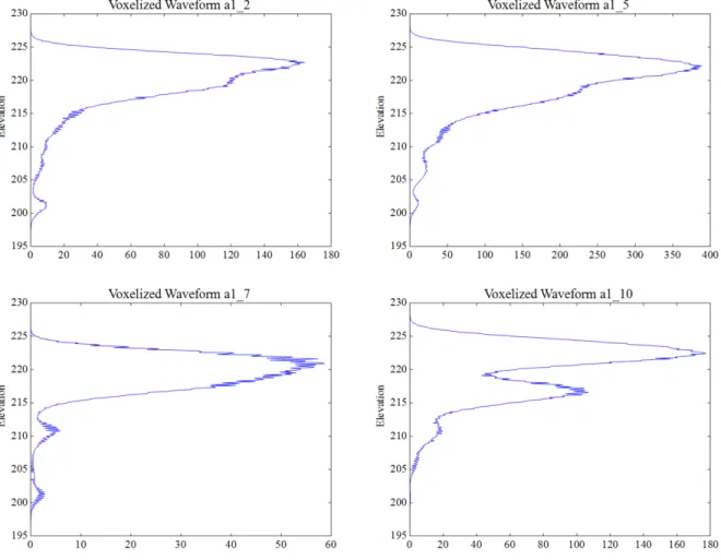
Using the tree delineated point cloud data, we find trees that match those that were sampled in the field. After extracting all waveforms for each sampled tree, we combine all waveforms associated with each tree using a voxelization method which allows up to capture vertical structure of biomass distribution [Hosoi and Omasa, 2006]. In this method, each tree is approximated as a cylinder. The height of the cylinder is the vertical range of the all waveforms in each tree, and the radius is the output from Envi-Lidar when using the discrete data as input for tree delineation. By dividing the cylinder into 1 cm layers, disk shaped voxels along the height of the tree are generated. Then by totaling all records that fall within each voxel, pseudo-waveforms, as shown in Figure 3.1, are generated for each tree. In order for each waveform to be comparable, each wave record is normalized with respect to the max intensity in the wave. The equation below demonstrates this process.

Vh =

X w_i

wmax

(3.1)

Vh is a voxel at a certain height,wi is a wave record, andwmax is the max intensity of the wave that contains wi.

3.1.2

Waveform Characteristics

To describe the pseudo-waveform for each tree, we chose several waveform structural char-acteristics listed below:

ˆ Total energy (tE). Total energy is the total area under the pseudo-wave of each tree. Found by integrating the wave with respect to elevation.

ˆ Total Height (tH). Total height is the vertical range of the pseudo-wave. The peak that likely represents ground return is not removed. Our reasoning is that the ground return characteristics below a tree is also an expression of tree structure. Dense trees are likely to have less significant ground return compared to foliage return, and the reverse is true for sparse trees.

ˆ Max energy (maxE). The maximum energy of the wave is the peak intensity value of the wave. In the case of the pseudo-waveform, this is the x-axis value (pseudo-intensity) shown in Figure 3.1. Due to normalizing the waveform, this value does not have a physical meaning, but is an indirect expression of the intensity of all waveforms for a tree.

ˆ Median energy (midE). The median energy is the median value of all pseudo-intensity values of the pseudo-waveform for each tree.

ˆ Relative height at 25% energy (RH25). RH25 is the relative height below which lies 25% of the pseudo-wave’s area. Integrating the pseudo-wave from minimum elevation to elevation at 25% results in 25% of total energy. Relative height entails a distance measurement that it is the elevation at 25% energy subtracted by the minimum pseudo-wave elevation.

ˆ Relative height at 50% energy (RH50). Similar to RH25, this is the height, relative to the minimum elevation, below which lied 50% of the pseudo-wave’s energy.

ˆ Relative height at 75% energy (RH75). Similar to RH25 and RH50, this is the height, relative to the minimum elevation, below which lied 75% of the pseudo-wave’s energy.

All wave characteristics above are calculated for the pseudo-waveform of each tree. Some are energy characters that describes the waveform intensity of each tree, and some are height characteristics that describes the pseudo-waveform structure and the distribution of energy. We believe this to be a thorough description of the different characteristics of the pseudo-waveform.

3.1.3

Field Biomass

In order to relate the pseudo-waveform characteristics described in the previous section to each tree’s biomass, we must have actual biomass values for some trees for guidance. We use field tree survey data and existing allometric equations to estimate biomass. There are many published allometric equations in existing literature. The National Biomass Estimator Library (NBEL) compiled many of them, and is a great tool for exploring tree biomass [Wang, 2014]. For each tree, the NBEL requires USDA forest service region code (09 for Illinois), DBH, tree height, and tree species as input. As a result, it returns biomass in kg for the tree calculated using all known allometric equations for the region. We then choose a reasonable number based on how suitable the original study is to the current situation. If a species of tree does not have an equation in this region, that of a similar tree, such as another type of maple for an unknown maple, is chosen.

Currently, since cutting down trees to measure biomass is no longer prevalent, biomass de-rived from allometric equations is generally accepted as valid biomass measurements. There-fore, even though these are estimations, we assume that the biomass results estimated from

field data are correct biomass values. Using the field survey data for the four sites mentioned in Chapter 2 Section 2.1.2, 33 usable trees are identified and above ground biomass, the mass of all vegetation above the ground, is calculated for each tree.

3.1.4

Regression

After estimating above ground biomass in the previous section for each surveyed tree, we can now relate each tree’s pseudo-waveform structural characteristics to its biomass through linear regression.

The simplest method would be to use multiple linear regression with each tree’s biomass as the dependent variable and the pseudo-waveform characteristics as explanatory, or in-dependent, variables. However, when we chose pseudo-waveform characteristics in Section 3.1.2, many of them describe similar traits. This leads to high cross correlation between explanatory variables, rendering all variables insignificant.

Therefore, we perform stepwise multiple linear regression between biomass estimated from field measurements and pseudo waveform structural characteristics using Matlabs Linear-Model. Stepwise regression builds a linear model, but repeatedly add or removed explana-tory variables based on a given criterion. Criterion used in this thesis is R2_{. Therefore, by}

using a stepwise regression we can filter out the least significant explanatory variables that may negatively influence the model fit. In order to check the validity of results, we only use 80% of trees, training data, as input to the stepwise regression model. The regression generates a model similar in the form to equation 3.2 shown below:

y∼1 +x1 +x2 +x1∗x2 (3.2)

Hereyis biomass, the dependent variable, and x1andx2 represent pseudo-waveform char-acteristics, the explanatory variables. To test the validity of the resulting model, the remain-ing 20% of tree data, test data, is used as input and the resultremain-ing biomass value is compared with the value derived from allometric equations.

3.2

Results

Since we choose a random 80% of data as regression input, the results of each repeated regression analysis are different. Figure 3.2 and 3.3 shows regression results for different

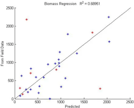
runs of the stepwise multiple linear regression. One outlier in the data had to be physically removed for reasonable results. In the model shown in Figure 3.2, the regression results are fairly good. The R2 _{value is not high by general standards, but is considered pretty good}

for this type of study. However, the R2 _{for the model shown in Figure 3.3 is extremely}

low. This unstable performance by the stepwise regression method is also evident in that each run results in a model based on different explanatory variables. In other words, we are not able to determine the most important pseudo-waveform structural characteristics that affects above ground biomass of each tree.

The variation in results from the regression analysis is likely due to the limited number of data points we have. Unfortunately, the inaccessibility of trees to measure due to dense understory is inevitable in dense forest as we have at USRB. Many other situations can also lead to limited amount of data. Since limited data is a prevalent problem, we then hope to test the effectiveness of statistical methods in finding significant explanatory variables. In order to determine the most significant pseudo-waveform structural characteristics that indicate biomass, we use a bootstrapping method and run the stepwise regression 500 times. Each time, the regression is applied to a randomly chosen 80% of the data as training data, and the remaining 20% is test data used as input to the resulting model which gives a predicted biomass value.

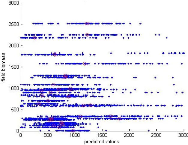
Figure 3.4 shows the results from the 500 runs of stepwise regression. The y-axis is the biomass of surveyed trees based on allometric equations and field data. The x-axis indicates biomass predicted by the model. Each blue point is a test data point, part of the 20% not used in building the model. Because the training data is chosen randomly, each surveyed tree has served as test data multiple times to different models. This leads to a horizontal spread of predicted biomass for each field measured biomass as shown in Figure 3.4. The red circles indicate the median value of all predicted biomass for each surveyed tree.

The model for each stepwise regression is also recorded and processed. In order to find the pseudo-waveform structural characteristics that has the most influence on biomass, we want to find the model that occurs most frequently from randomly chosen training data. Out of 500 runs, there are 149 unique models. By our definition, two models are the same if they used the exact same explanatory variable and operations between variables. For example,

y ∼ x1 + x2 is the same as y ∼ x2 + x1. Their coefficients may differ. The model that occurred most frequently is:

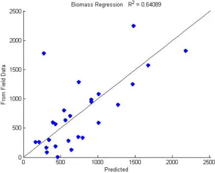
which occurred 33 time out of 500. This model is relatively simple and only uses two terms, tE and RH50. Figure 3.5 shows biomass prediction results of using only tE and RH50 as explanatory variables. In this case, R2 _{value is based on all data instead of just the test}

data.

Closely following the model shown in Equation 3.3 in terms of frequency of occurrence are:

Biomass∼1 +midE +tE+RH50 +tE ∗RH50 (3.4)

Biomass∼1 +tE +tH +tE ∗tH (3.5) which occurred 32 and 31 times respectively. The model shown in Equation 3.4 is very similar to that of Equation 3.3. The only difference is the addition of the linear midE term. The model in Equation 3.5 is similar in form to that of Equation 3.3. The difference here is the used of tH instead of RH50, which are both height terms. tE occurred in all three models. RH50 occurred in two. midE and tH each occurred once.

3.3

Figures

Figure 3.2: Example of relatively well fitted model. Model based on randomly chosen 80% of data. Blue points are data used in the regression. Red points are the remaining 20% test data. R2 _{value is based on test data only.}

Figure 3.3: Example of poorly fitted model. Model based on randomly chosen 80% of data. Blue points are data used in the regression. Red points are the remaining 20% test data.

Figure 3.4: Biomass results from stepwise regression combined with bootstrapping. All test data are shown in blue. Red circles show the median of all predicted biomass for each tree.

Figure 3.5: Biomass prediction results using the most prevalent model from 500 bootstrap runs shown in Equation 3.3.

CHAPTER 4

FOLIAGE CLUMPING

In this Chapter we propose an easily scalable method to estimate physical canopy clumping structure for individual trees using airborne full-waveform LiDAR data. Canopy clumping is hard to quantify, since what entails a clump can be subjective. Traditionally clumping indices are used to describe the amount of clumping on a large scale. These indices are generally derived using optical tools such as hemispherical photos.

Using airborne LiDAR data will not only provide wide coverage, but can potentially give a fine scale description of the canopy clumping characteristics that clumping indices cannot provide. In this Chapter, we attempt a new method that describes clumping structure in waveform LiDAR data, which should give an indication of actual canopy clumping.

We first describe our method used for clustering the waveform data, then we present the clustering results. Interpretations of the clustering results and conclusions will be described in Chapter 6 and 7.

4.1

Methods

In this section we describe why we choose to use K-means clustering, and how we use simulated LiDAR data test the most applicable method of finding the K in K-means. Then we present how we cluster the records (each recorded intensity) in the waveform LiDAR data and our clustering results for a sample tree selected from USRB.

4.1.1

Cluster by K-means

Waveform LiDAR data can provide detailed canopy structural information. However, the relation between individual waveforms and records in each waveform is unknown. In order to find patterns in the LiDAR data, clustering analysis can be extremely useful [Jain, 2010].

Clustering is a form of unsupervised pattern recognition involving only unlabeled data, such as our waveform LiDAR records [Duda et al., 2012]. The purpose of data clustering is to find the natural groupings of a set of data, or points, in order to gain insight into the underlying structure of the data set. Clustering characteristics in LiDAR data can help us gain insight into canopy foliage clumping.

Cluster analysis is an extremely useful but also difficult process due to the subjective na-ture of the problem. This challenge has led to an increasing number clustering algorithms [Jain, 2010]. Two main categories of clustering algorithms are hierarchical and partitional. Hierarchical clustering recursively combines or divides clusters while partitional clustering divides the data into a set number of clusters simultaneously. The more resource intensive hi-erarchical clustering is unsuitable for the large amount of waveform LiDAR data. Therefore, K-means, a widely used partitional clustering algorithm, is chosen.

K-means is one of the most popular clustering algorithms due to its simplicity, efficiency, and empirical success [Jain, 2010]. The algorithm seeks to minimize the sum of the squared errors (SSE) of all clusters shown in Equation below [Jain, 2010]:

J(C) = K X k=1 X xck ||x−µk||2 (4.1)

Here, K is the total number of cluster, ck represents one cluster, and µk is its center. Given K, a distance metric (usually Euclidean distance), and a cluster initialization method, the K-means algorithm first partitions the data into K clusters according to the given initialization method. Next, it re-clusters by assigning each data point to its closest cluster center based on the given distance metric. Using cluster centers from new clusters, re-clustering is repeated until clusters are stable [Jain and Dubes, 1988].

In this thesis, four features for each data point are selected as input to the K-means clustering algorithm, xyz location based on UTM N16 and record intensity. Point location serves to group points of close spatial proximity. Intensity is used to group points of similar return characteristics. In order to only use the most informative data, all records with intensities below half of the max intensity of their respective peaks are removed. Intensities are then linearly scaled so that the max value is the range of elevation. Scaling is necessary for comparability between variables. We use Euclidean distance as the distance metric and use randomly selected data points as initial cluster centers.

4.1.2

Cluster Evaluation

The challenge in using K-means clustering is choosing the correctK, the number of clusters, since what constitutes the correct number of clusters may be subjective [Han et al., 2011]. OftenK is determined through trial and error and there may be no justification for selecting a particular value [Pham et al., 2005]. However many methods exist for selecting the K in K-means. In this thesis, we consider many representative methods for choosing K. These include:

ˆ Nominal K [Kodinariya and Makwana, 2013]. The nominal K is a rule of thumb for selecting K given by Equation 4.2 below:

K ≈pn/2 (4.2)

It is only based on the total number of data points being clustered by the K-means algorithm. Therefore it may not be applicable in all situations. However, it does give a large enough K estimate in our case to ensure we are not over simplifying data structure.

ˆ Elbow Method [Ng, 2012]. The elbow method is a traditional method for estimating

K in K-means. In this method, clustering results are evaluated by the SSE shown in Equation 4.1. K-means is run for a range of K values, and the SSE is calculated for each clustering result. The calculated SSE is then plotted against their respective K

values. In an ideal case, the resulting plot shows a curve with a sharper bend in the middle, looking like a bent arm. The K value where the curve bends the sharpest, the elbow, is the correct K to use for K-means.

ˆ Calinski-Harabasz or Pseudo-F Index [Cali´nski and Harabasz, 1974]. Similar to the elbow method, finding the correct number of clusters, K, to use using the Pseudo-F index also requires running the K-means algorithm for a range of K values. In this case, the Pseudo-F Index, shown below is used to evaluate cluster results instead of the SSE.

P seudoF = BGSS/(K−1)

W GSS/(N −K) (4.3)

Here BGSS is the between group sum of squares, and W GSS is the within group sum of squares. BGSS is calculated as the squared error of all cluster centroids, and

W GSSis the SSE of the clustering result. N is the total number of data points, andK

is the number of clusters. This index is named Pseudo-F index because it is analogous to the F-statistic used by Edwards and Cavalli-Sforza [1965] in cluster analysis. Larger values indicate tighter and more separated clusters. Ideally a goodK value is indicated by peaks in the plot of this index with respect to the number of clusters [Wilkinson et al., 2012].

ˆ Silhouette Score [Kaufman and Rousseeuw, 2009]. The Silhouette Score is the mean Silhouette Coefficient or all clusters. This index should also be calculated for clustering results from a range of K values. The equation for calculating Silhouette Coefficient for each cluster is shown below:

Silhouette= b−a

max (a, b) (4.4)

Here a is the mean within cluster distance, or the mean distance between all pairs of data points in a cluster. b is the mean nearest-cluster distance, or the mean distance from all points in the cluster to the nearest point that is not in the cluster. This coefficient measures how cohesive each cluster is and how separate it is from neighboring clusters. As we can tell from Equation 4.4, the coefficient ranges from -1 to 1. Larger value indicate more distinct clusters. A suitable value of K can be chosen using the plot of the Silhouette Score, mean Silhouette Coefficient for all cluster, with respect to

K, the number of clusters.

ˆ Bayesian Information Criterion (BIC) [Pelleg et al., 2000, Schwarz et al., 1978]. The BIC used in Pelleg et al. [2000] as the stopping criteria for the x-means algorithm, which is simply an accelerated K-means clustering that chooses K automatically based on BIC. The Bayesian Information Criterion, also called the Schwarz Criterion, is first used by Schwarz et al. [1978]. Since then, many form of the criterion has developed. The following equation comes from Wit et al. [2012].

BIC =−2l(ˆθ) +plog(N) (4.5) Here, l(ˆθ) is the maximum log likelihood of all clusters, pis the number of parameters in the clustering data, four in our case. N is the total number of data points. The BIC measures the posterior probability as an evaluation of a clustering result. Using

Equation 4.5, minimizing BIC gives the maximum posterior probability. By evaluating clustering results for a range ofK values using BIC, the correctK should ideally occur at the minimum BIC value.

ˆ Dunn’s Index [Dunn, 1973]. This is another cluster evaluation index that measures the compactness within clusters and separation between clusters. It is defined as the minimum Euclidean distance between any two points in the data set that belongs to different clusters. DIK = min 1≤i<j≤Kδ(ci, cj) max 1≤h≤K∆h (4.6)

where the numerator is the minimum Euclidean distance between any pair of cluster centers, and the denominator is the maximum diameter of any cluster. Here ∆h, the diameter of a cluster, is defined as the maximum distance between any two points in the cluster. It is a measure of the spread of data in a cluster. It can also be define as the mean distance between all data pairs in a cluster (same as a in Equation 4.4) or the mean distance between each point and its respective cluster center. Larger Dunn’s index indicates more tightly grouped clusters.

ˆ Minimum Between-cluster Distance (minBdist). The minimum between cluster dis-tance is an additional index used in this thesis to test for the correct K value in K-means clustering. The reasoning behind using this measure to evaluate clustering results is that asK value increases, larger clusters are, ideally, being divided into more tightly grouped smaller ones. Therefore, when K is small, the minBdist should be large, and as K increase, minBdist should become gradually smaller until it reaches the minimum distance between any two data points. Ideally the correctK value should be when the minBdist starts to decrease more slowly, indicating that any more increase inK will result in dividing more tightly grouped clusters.

ˆ Minimum Center Distance (minCdist). The minimum center distance is also another index developed in this thesis to estimate the correct K value when K-means is ap-plied to LiDAR data. This index measures the minimum distance between any two cluster centers. The reasoning and expected behavior of minCdist is similar to that of minBdist. When K is small, there should be few clusters where cluster centers are far apart. As K increase, minCdist should also become gradually smaller since there

are more and more small clusters. Ideally the correct K value should be when the minCdist starts to decrease more slowly. This should be an indication that additional increase in K will result in dividing tightly grouped small clusters.

4.1.3

Point Cloud Simulation

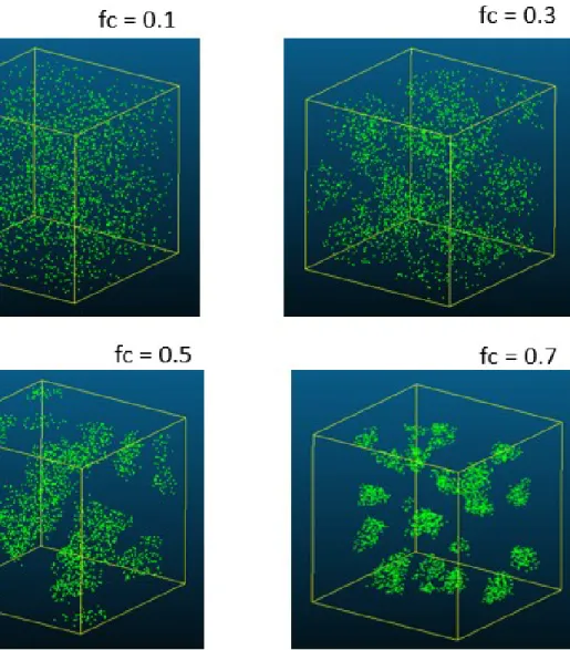
We test the applicability of each method of choosing K mentioned above using simulated LiDAR point clouds with given degree of foliage aggregation and known number of clusters. Similar simulation procedures has been used by [de Castro and Fetcher, 1999], then [Walter et al., 2003]. In these previous works, LAI is needed as input to simulate foliage canopy. In this thesis, the number of points in the discrete LiDAR point cloud of an area of interest (Np) is used instead of LAI to represent the amount of foliage in the canopy. Additional parameters needed as input include the number of clusters (Nc), and the cluster percentage (fraction clumping,Fc). Fcis a fraction between 0 and 1 used to scale the distance between each point and its closest cluster center. To generate a point cloud with given degree of foliage aggregation, the first step is to generate Np points randomly distributed within the same volume as that of the original point cloud. Then Nc cluster centers are also randomly located within the volume. Each of theNp points in the point cloud is displaced toward its closest center according to

d0 = (1−Fc)d (4.7)

The displacement of each point occurs along the vector between the point and its closest center. d is the original length of the vector, and d0 is the distance after displacement. As should be clear from Equation 4.7 above,Fc= 0 corresponds to a completely random canopy, and Fc= 1 represents a completely compacted one.

4.1.4

K for Simulated Point Clouds

Once a point cloud with a given number of clusters is simulated, we test the applicability of each cluster evaluation index by repeatedly clustering the point cloud using increasing number of clusters (K). Each cluster result is tested with the cluster evaluation methods mentioned in Section 4.1.2, and an index is generated for each given K. This testing process

is run multiple times, and an average index from all runs for each K is used to judge the performance of the cluster evaluation method.

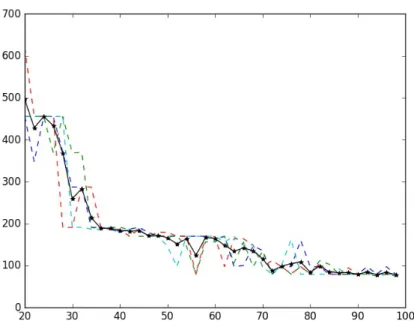
Most cluster evaluation methods mentioned in Section 4.1.2 are unable to correctly identify the number of clusters in the simulated point clouds. Figure 4.2 and 4.3 shows examples of failed cluster evaluation methods. Figure 4.2 shows the results from using BIC as cluster evaluation index on a simulated point cloud with 60 clusters and Fc of 0.6. A range of K values are used to cluster the point cloud and BIC is calculated for each cluster result. In the resulting line plot, the BIC decreases with increasedK, indicating better clustering, however, it shows no sign that K = 60 is any better than otherK values in that range. Therefore, we cannot use BIC as a cluster evaluation for waveform data clustering when looking correctK. Another example of a failed cluster evaluation index is minimum between cluster distance. This index is applied to a simulated point cloud with similar parameters as that of the BIC test, 60 clusters and Fc of 0.6. Again a range of K values are used for clustering. The plot of minBdist with respect toK is shown in Figure 4.3. Similar to BIC, this evaluation index give no indication that the clustering result of K = 60 is any different from others in that range. Based on the results, we would most likely choose K = 45, which does not agree with the actual number of clusters.

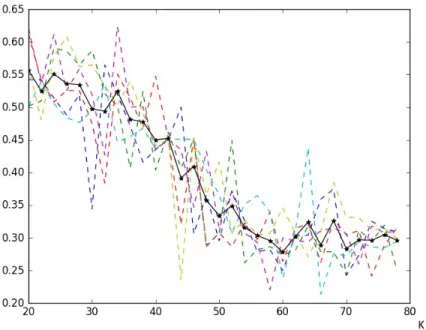
Only two of the cluster evaluation methods mentioned in Section 4.1.2 yields promising results. One is the Dunn’s index described by Equation 4.6. The Dunn’s index is also used for evaluating clustering for a simulated point cloud with 60 clusters and Fc of 0.6. The results are shown in Figure 4.4. In theory, larger Dunn’s index indicates tighter clustering. However, the index gradually decreases for increasing number of clusters until the K grows past the correct cluster number. This method may not be suitable for evaluating cluster validity given the index value at the correct number of clusters, it does indicate when the correct number is reached by comparing multiple runs of K-means clustering.

Another cluster evaluation measure that yields good results is the minimum center distance described in Section 4.1.2. This measure is simply the numerator of Dunn’s index, and its behavior is similar as well. However, it is significantly smoother compared to the Dunn’s index as shown in Figure 4.5. From the Figure, it is easy to see that the correct cluster number occurs after the bend in the graph. The measure generally remains constant with increasing K after that.

4.1.5

K for Waveform Data

The cluster evaluation methods that performed well with the simulated point clouds, Dunn’s index and minCdist, is then applied to the waveform data of the tree of interest. Results are shown in Figure 4.6. Cluster evaluation results for the waveform data do not show as strong indication of the correct cluster number as previous simulations. We believe this might be due to higher point densities in the waveform data as well as less distinct clusters. However, the results still shows similarities. In the results for Dunn’s index, shown in Figure 4.6a, the index decreases at first, but seems to reach a plateau afterK = 130. There seems to be another plateau after K = 210. However, the large variations in the index value after this point prevents any conclusive decisions.

The results from the minimum cluster center distance measure, shown in Figure 4.6b are also inconclusive. With this measure, we encounter the same problem which plagues the oldest method for determining K in K-means, the elbow method [Ng, 2012]. Similar to the ideal elbow method result, the result from the minimum cluster center distance measure has a distinct bend, or elbow, at the correct number of clusters. However, often times there is no distinct bend in the result from the elbow method, as is the case with our measure and the waveform data. In this situation, we can only specify a range that the correct K is likely to be in. From Figure 4.6b, the range 100< K < 250 seems to be the center section of the elbow.

In such ambiguous situations, several K values can be used [Pham et al., 2005]. In this study, we choose to use K = 130 and K = 220. These numbers are close to the likely K values from the evaluation using Dunn’s index, they also represent the range of K identified in the minimum center distance measure. Also,K = 220 is chosen because it also corroborates with the rule of thumb for selecting K defined as follows where n is the number of data points.

4.2

Results

Waveform data for an individual tree is extracted, and all records in each waveform are converted to points in space. The K-means clustering algorithm is then applied to the waveform data using K = 130,220. The tree used and the cluster results are shown in Figure 4.7.

ˆ Average Cluster Intensity. The average intensity of all records in each cluster. Results are shown in Figure 4.8. Clustering results for both K value are very similar to the unclustered intensity data shown in Figure 4.7a.

ˆ Cluster Count. The number of records in each cluster. Results are shown in Figure 4.9. There are slight differences for the cluster results from differentK values. Clusters for

K = 220 have less variation in the number of records per cluster.

ˆ Cluster Volume. The volume of each cluster calculated by fitting a convex hull around all points. Results are shown in Figure 4.10. The most notable result is that data for the tree canopy form significantly larger clusters than data representing the ground.

ˆ Cluster Diameter. The maximum distance between any two points in the cluster. Results are shown in Figure 4.11. The results for K = 220 have many blue, or small diameter, clusters. This indicates that there are many small clusters and a few large clusters. Results for K = 130 seems more evenly distributed with small, medium and large clusters.

Cluster volume and cluster diameter are both measures of the spread of a cluster. Clusters with larger diameter should theoretically have larger volume. As expected, we find that they exhibit a strong positive correlation shown in Figure 4.12. Therefore, cluster volume is not used for further analysis. Figure 4.13 shows the distribution of values for the three remaining cluster traits. We can see that their distribution are very similar. This leads us to believe the K values we chose are in the correct range for describing the data structure.

By plotting the three remaining traits, intensity, count, and diameter, using a 3D scatter plot, we see distinct groups form in the traits data. To classify these groups, we also use the K-means algorithm (the term ’groups’ is used to describe to cluster traits to distinguish from ’clusters’ of the waveform data). First, the three sets of trait data for all clusters are normalized so that the maximum of each set is one. Then each cluster, each with three traits, is used as a data point as input to the K-means algorithm. This time, to find the optimal number of groups we apply the Dunn’s index to evaluate and compare K-means grouping results as shown in Figure 4.14. From observation the we believe the traits data best fit into three groups. However, according to Dunn’s index, dividing the data into 2 or 4 groups result in the best groups. Because 2 groups might not adequately describe the structure in the traits data, K-means is performed using 4 groups. Results are shown in Figure 4.15. By observation, we can tell that the groups colored blue and black in Figure 4.15 can be

considered one group. Because the K-means algorithm is more suitable for spherical clusters, this elongated cluster in the data was split in two.

Judging from only three groups, where the blue and black groups are grouped into one, there are several noticeable trends in the traits data. Most noticeably, is that there are very few differences between results using K = 130 andK = 220. This can be an indication that the Ks are chosen in the correct range. In terms of the traits data, the elongated group (colored blue and black) is noticeably separate from the rest of the data. This group have very low intensity and low diameter. Their count is relatively high but varies. This means that these low intensity clusters are small and dense. There are also more data points in this group when compared with the others. The remaining traits data is split into two groups. In these data, cluster average intensity is positively correlated with cluster diameter, but negatively correlated with the cluster count, the number of data points in the cluster. This indicates that data clusters with high intensity, the red group in Figure 4.15, are large but with sparse data points. There are also the fewest clusters in this group. Compared to the red group, green group contains clusters with lower intensity, smaller diameter and higher count. These clusters, similar to those in the elongated group, are also small and dense, but have significantly higher intensity.

In summary, foliage clumping can be physically described by clustering waveform LiDAR data. Each cluster is described by three traits: average cluster intensity, number of data points, and cluster diameter. By using these traits, clumps in vegetation can be grouped into three main groups

ˆ Group 1. Low intensity group that are small and dense. A majority of clusters fall in this group

ˆ Group 2. Medium intensity group that are also small and dense. There are relatively less clusters in this group

ˆ Group 3. High intensity group that are large but sparse. This groups contains the fewest number of clusters

Of the three groups, group 1, with low intensity, contains the least amount of clumping information. Waveform data clusters in this group might have resulted from few scattered leaves or ascending and descending edges of the return laser waveform due to a foliage clump. Group 2, with clusters similar in size and density to those of group 1, have significantly higher intensity. They likely represent slightly denser foliage or small foliage clumps. Group

3 provides the most information on the structure of the canopy due to foliage clumping. Clusters in this group have high intensity, indicating strong returns, likely from dense foliage clump with few to no gaps. Also, since here should be fewer returns in dense areas, the sparse data of clusters in group 3 is also indicative of dense vegetation.

4.3

Figures

Figure 4.2: K-means cluster evaluation by BIC using a simulated point cloud with 60 clusters. The solid line represents the average of all repeated runs which are shown as dashed lines.

Figure 4.3: K-means cluster evaluation by minBdist using a simulated point cloud with 60 clusters. The solid line represents the average of all repeated runs which are shown as dashed lines.

Figure 4.4: K-means cluster evaluation by Dunn’s index using a simulated point cloud with 60 clusters. The black line represents the average of all repeated runs, shown as colored lines.

Figure 4.5: K-means cluster evaluation by minimum cluster center distance using a simulated point cloud with 60 clusters. The black line represents the average of all repeated runs, shown as colored lines.

Figure 4.6: K-means cluster ev alu ation b y a. Dunn’s index and b. minim um cluster cen ter distance using the w a v eform LiD AR data of a tree. The blac k line represen ts the a v erage of all rep eated runs, sho wn as colored lines.

Figure 4.7: a. W a v eform data of the tree where high in tensit y sho ws as green and lo w as blue; b,c. Cluster results for K = 130 and K = 220, eac h color represen ts individual clusters.

Figure 4.8: Cluster results for K = 130 and K = 220 colored b y cluster in te nsit y. Blue is le ss in tense, and red the most in tense.

Figure 4.9: Cluster results for K = 130 and K = 220 colored b y cluster coun t. Blue means less records, and red is more records p er cluster.

Figure 4.10: Cluster v olume for K = 130 and K = 220. Blue represen ts smaller clusters, and red represen ts larger clusters.

Figure 4.11: Cluster diamete r results for K = 130 and K = 220. Blue is smalle r diameter, and red is larger diameter.

Figure 4.12: Relationship between cluster diameter and cluster volume. Each point represents a cluster found by K-means.