Does Class Size Matter? How, and at What Cost?

Economics Working Papers

4-2019

Does Class Size Matter? How, and at What Cost?

Does Class Size Matter? How, and at What Cost?

Desire Kedagni

Iowa State University, [email protected] Kala Krishna

The Pennsylvania State University Rigissa Megalokonomou University of Queensland Yingyan Zhao

The Pennsylvania State University

Follow this and additional works at: https://lib.dr.iastate.edu/econ_workingpapers

Part of the Education Policy Commons, Labor Economics Commons, and the Public Policy Commons

Recommended Citation Recommended Citation

Kedagni, Desire; Krishna, Kala; Megalokonomou, Rigissa; and Zhao, Yingyan, "Does Class Size Matter? How, and at What Cost?" (2019). Economics Working Papers: Department of Economics, Iowa State University. NBER 25736.

https://lib.dr.iastate.edu/econ_workingpapers/87

Iowa State University does not discriminate on the basis of race, color, age, ethnicity, religion, national origin, pregnancy, sexual orientation, gender identity, genetic information, sex, marital status, disability, or status as a U.S. veteran. Inquiries regarding non-discrimination policies may be directed to Office of Equal Opportunity, 3350 Beardshear Hall, 515 Morrill Road, Ames, Iowa 50011, Tel. 515 294-7612, Hotline: 515-294-1222, email

[email protected].

This Working Paper is brought to you for free and open access by the Iowa State University Digital Repository. For more information, please visit lib.dr.iastate.edu.

Does Class Size Matter? How, and at What Cost?

Does Class Size Matter? How, and at What Cost?

Abstract Abstract

Using high quality administrative data on Greece we show that class size has a hump shaped effect on achievement. We do so both nonparametrically and parametrically, while controlling for potential endogeneity and allowing for quantile effects. We then embed our estimates for this relationship in a dynamic structural model with costs of hiring and firing.

We argue that the linear specification form used in past work may be why it found mixed results. Our work suggests that while discrete reductions in class size may have mixed effects, discrete increases are likely to have very negative effects while marginal changes in class size would have small negative effects. We find optimal class sizes around 27 in the absence of adjustment costs and achievement maximizing ones around 15, and firing costs much larger than hiring costs consistent with the presence of unions. Despite this, reducing firing costs actually reduces achievement. Reducing hiring costs raises

achievement and reduces class size. We show that class size caps are costly, and more so for small schools, even when set at levels well above average.

Disciplines Disciplines

NBER WORKING PAPER SERIES

DOES CLASS SIZE MATTER? HOW, AND AT WHAT COST? Desire Kedagni Kala Krishna Rigissa Megalokonomou Yingyan Zhao Working Paper 25736 http://www.nber.org/papers/w25736

NATIONAL BUREAU OF ECONOMIC RESEARCH 1050 Massachusetts Avenue

Cambridge, MA 02138 April 2019

The views expressed herein are those of the authors and do not necessarily reflect the views of the National Bureau of Economic Research.

NBER working papers are circulated for discussion and comment purposes. They have not been peer-reviewed or been subject to the review by the NBER Board of Directors that accompanies officialNBER publications.

© 2019 by Desire Kedagni, Kala Krishna, Rigissa Megalokonomou, and Yingyan Zhao. All rights reserved. Short sections of text, not to exceed two paragraphs, may be quoted without

Does Class Size Matter? How, and at What Cost?

Desire Kedagni, Kala Krishna, Rigissa Megalokonomou, and Yingyan Zhao NBER Working Paper No. 25736

April 2019

JEL No. C61,I20,I28,J48

ABSTRACT

Using high quality administrative data on Greece we show that class size has a hump shaped effecton achievement. We do so both nonparametrically and parametrically, while controlling for potential endogeneity and allowing for quantile effects. We then embed our estimates for this relationship ina dynamic structural model with costs of hiring and firing.

We argue that the linear specification form used in past work may be why it found mixed results. Our work suggests that while discrete reductions in class size may have mixed effects, discrete increasesare likely to have very negative effects while marginal changes in class size would have small negativeeffects.

We find optimal class sizes around 27 in the absence of adjustment costs and achievement maximizing ones around 15, and firing costs much larger than hiring costs consistent with the presence of unions. Despite this, reducing firing costs actually reduces achievement. Reducing hiring costs raises achievement and reduces class size. We show that class size caps are costly, and more so for small schools, evenwhen set at levels well above average.

Desire Kedagni Iowa State University Department of Economics

467 Heady Hall, 518 Farm House Lane Ames, IA 50011-0154

[email protected] Kala Krishna

Department of Economics 523 Kern Graduate Building The Pennsylvania State University University Park, PA 16802 and NBER [email protected] Rigissa Megalokonomou Department of Economics University of Qeensland [email protected] Yingyan Zhao

The Pennsylvania State University

1 Introduction

What determines student achievement? The usual approach is to think of achievement as the output of an educational production function. Inputs into this educational production function include teacher quality, class size, resources, peer eects (possibly positive spillover eects and negative disruption eects), as well as past achievement since achievement builds on the past knowledge.

In this paper, we focus on the eects of class size on achievement. This area has been widely studied in both labor economics and education. Somewhat surprisingly, the estimates are relatively mixed. A recent paper, Leuven et al.(2008) summarize the state of the debate as follows:

One of the still unresolved issues in education research concerns the eects of class size on students' achievement. It is by now well-understood that endogeneity problems may severely bias naive OLS estimates of the class size eect, and that exogenous sources of variation in class size are key for a credible identication of the class size eect. Various recent studies acknowledge this and apply convincing identication methods. This has, however, not led to a denite conclusion about the magnitude or even the sign of the class size eect.

While performance has been related to class size, there has been little attempt to allow for nonmonotonicities.1 _{For example, it could be that larger class size rst raises (as students learn}

from each other as well as the teacher) and then lowers achievement (when congestion eects take over). In this paper, we explicitly allow for such possibilities. We argue that not allowing for nonmonotonicities could be why the literature has found mixed results.

We use high quality administrative data on Greece to rst show nonparametrically that there does indeed seem to be such a hump shape in the data. Following this, we estimate a parametric relationship between class size and achievement while carefully dealing with issues of endogeneity of class size. We show that class size does matter and that the linear specication form used in past work may be why past results were mixed. After all, if we t a linear regression when the true relationship is quadratic, we could get a positive, negative or zero slope depending on the precise shape of the underlying true quadratic relationship. Our estimates suggest that the shape of this relationship is relatively at in the relevant region, namely the region close to the chosen class size. As a result, a marginal reduction in class size can have a small positive eect on achievement. Moreover, as the chosen class size, in the presence of adjustment costs, will exceed the class size at which achievement is maximized, a large reduction in class size could easily move achievement

to the other side of the hump and have little or no eect on achievement. For these reasons, the eect of increases versus decreases in class size can be very asymmetric. All of this is consistent with what the literature has found: namely that decreasing class size is a costly way of raising achievement.

We further explore the data to look for evidence of quantile eects. We nd that the hump shape is present across all quantiles, i.e., for students of all abilities. The hump shape is however more pronounced for worse students.

This paper proceeds as follows. In Section 2, we put our work in perspective relative to the literature. In Section 3, we describe where the data came from, present some summary statistics and descriptive regressions. In Section 4, we present the rst nonparametric evidence of a hump shaped relationship in class size and achievement. In Section 5, we take a parametric approach and use the Hoxby instrument, see Hoxby (2000), to control for endogeneity. In Section 6, we present our quantile IV results.

With the estimates of the eects of class size on achievement in hand, we are in a position to understand how class size is chosen. If the government cares about achievement, and faces costs of adding classes, its behavior in terms of the number of classes it chooses as enrollment uctuates helps us estimate the costs involved. We use our reduced form estimates in a dynamic structural model of class size to estimate hiring/ring and marginal cost of adding a class. Our estimates here are in line with actual teacher salaries. Finally, in Greece, as in much of the rest of the world, teachers unions are a powerful force to be reckoned with. Their power is expressed not only in terms of wages set but in terms of the ability to re teachers at will. We use the model to ask whether inexibility in terms of unions creating high ring (and even maybe hiring) costs might be driving class size choices by government and the impact of this on student achievement if any. We nd that unions, even if they raise costs and class size, have a small eect on achievement. Finally, we look at the costs versus benets of class size requirements. Section 7 concludes.

2 Relation to the Literature

Given the increasing importance of skills in the labor force in the age of robotics and articial intelligence, there is intense interest in what drives educational attainment. A small part of this debate has focused on the role of class size on achievement. An excellent, though slightly dated survey can be found in Hanushek (2003) and Rivkin et al.(2005).

The main problem is that class size itself is a choice, i.e., it is highly endogenous. Teach-ers and headmastTeach-ers are better informed about students than the econometricians. Based on

students' characteristics that the econometricians do not observe, headmasters tend to allocate better students to larger classes, thus generating a positive correlation between class size and stu-dent performance. As a result, OLS estimates of the coecients on class size cannot be interpreted causally. This is not a problem specic to class size, but is more general. For example, estimat-ing eects of other school inputs on pupil outcomes is also complicated by potential endogeneity issues.2 _{The usual way to deal with this problem is to have a good instrument or an experiment}

and this is essentially the route the literature has taken as described below.

The best known experiment is the Tennessee STAR experiment. Students were randomly assigned to dierent sized classes. This should make it straightforward to estimate at least the policy eect of class size. However, there remain concerns about whether teacher quality changed, and the attrition and entry of students throughout the experiment (which could also have been endogenous) could confound the results (Hoxby, 2000; Hanushek, 1999). Krueger (1999) and

Krueger and Whitmore (2001) nd that smaller class sizes in kindergarten and rst grade seemed

to have a signicant and lasting positive eect on academic achievement.

More recently, Jepsen and Rivkin (2009) study California's class size reduction program for grades K-3. This reduced class size on average from 30 to 20 at a cost of roughly a billion dollars. They nd this policy raised math and reading achievement by roughly .10 and .06 standard deviations of the average test scores respectively, holding other factors constant. This is about the same eect as that of having a teacher with two more years of experience. Assuming teachers' salaries rise at less than 15% per year of experience, class size reductions would seem the more expensive option.3 _{Chetty et al.(2014) shows that teacher quality measured as value added has a}

huge eect on outcomes. Using U.S. data on over a million primary school children, he shows that replacing a teacher in the lowest 5% of value added with the average teacher would have signicant positive eects on outcomes like college attendance and teenage pregnancy and increase the lifetime earnings of the students in a classroom by $250,000.

In contrast to much of the work using eld experiments above, an elegant and often used quasi experimental approach is based on class size limits which turn out to be relatively common.

Angrist and Lavy (1999) noticed that in Israeli public schools, by law, there could be no more

than 40 students in a class. Thus, if a cohort grew beyond 40, there would be an exogenous fall in class size from 40 to 21, while if the cohort grew over 80, there would be an exogenous fall in class size from 40 to 27, and so on. They show that without correcting for endogeneity, class size

2_{School inputs are chosen by parents, school administrators, teachers, and politicians at both local and national}

levels. For instance, parents locating close to resource abundant schools may have chosen to locate there because they care a lot about their children's education and so also invest more time in their children's education (creating a upward bias).

seems to be positively associated with achievement, but when endogeneity is controlled for the sign is reversed. This makes economic sense as when students are good, larger class sizes can be tolerated which will bias OLS estimates upwards. Their estimates are for grades 3, 4 and 5. The coecient on class size is not signicant for grade 3, but is signicantly negative for grades 4 and 5. In general, estimates suggest that class size is a costly way of improving achievement.

Other papers which exploit maximum class-size rules includeBonesrønning(2003) for Norway,

Urquiola (2006),Browning and Heinesen(2007) andBingley et al.(2007) for Denmark. Browning

and Heinesen (2007) focus not only on class size but also on teacher hours per student. The class

size is limited to 28 students in Denmark. However,Bingley et al. (2007) nd that the target class size in the data seems to be closer to 24 suggesting that the limit is not binding and the quasi experimental approach is invalid.

The other approach to correct for endogeneity of class size is related to the work of Hoxby

(2000). In the absence of binding class size limits, one might think of using variations in overall enrollment as exogenous shocks. Hoxby goes a step further: she ts a quartic to the enrollment data and uses deviations from the quartic as the exogenous variation. In this way, she controls for trends in enrollment.

Gary-Bobo and Mahjoub (2013) use data on French junior high schools and Urquiola (2006)

use Bolivian data and follow Hoxby's approach. Though the estimated causal eects of larger class size tend to be negative, they remain small. In the context of the literature, our approach follows

Hoxby (2000). In our work, as there is no explicit class size cap, we cannot use the Angrist and

Lavy approach. As a result, we use Hoxby's instrument.

Levin(2001) andDobbelsteen et al. (2002) use a third source of quasi experimental variation.

They use PRIMA data. This longitudinal survey of Dutch students in grades 2,4, 6 and 8 in 1994-5 is rich in information including IQ as well as a new instrument for class size. Dutch rules link the number of teachers that can be hired to enrollment and this provides quasi exogenous variation in the number of classrooms. Levin explores peer and quantile eects. Dobbelsteen et al. (2002) also nd strong peer eects on student achievement. Controlling for peer eects, they nd class size eect to either be insignicant or signicantly negative.

Even with a good experiment, the literature has made a clear distinction between interpreting the coecients as structural parameters (i.e., the causal eect of class size) and policy estimates (i.e., the expected eect of an exogenous policy on class size). For example, suppose we changed class size experimentally (so that one group of students was in large classes and another was in small classes) and parental behavior responded to these changes, the estimated eects would be compound eects including the pure eect of changing class size and the induced one on parental

behavior. Todd and Wolpin (2003) in particular emphasize that estimates of the class-size eect even using experimental data should be interpreted as policy eects. In contrast, estimates aimed at identifying structural parameters of the education production function could be interpreted as the pure eect of class size, if other channels, like parental inputs in the example above, are accounted for.

It is worth noting that we could nd only two papers that allowed for nonmonotonic eects.

Borland et al. (2005) uses data from the Kentucky Department of Education for the third grade

in 1989-90. They specify a four-equation simultaneous equation system. Class size, achievement, market competition and teacher salary are the endogenous variables and achievement is allowed to be a quadratic function of class size. They argue that class size and GPA could be nonmonotonic. Why? Students learn from peers like themselves and the larger the class, the more likely it is that they have peers like themselves and GPA rises with class size. On the other hand, there is crowding and ultimately these congestion forces dominate so that GPA rst rises with class size and then falls which is what they nd. There are a number of issues with the paper. First, the economic model behind their simultaneous equation system and the exclusion restrictions used is far from clear. Second, their estimates are dicult to reconcile with their data patterns. Their estimates suggest a peak of achievement around class size 26. If class size was being chosen to maximize achievement subject to costs, the optimal class size must be to the right of the peak of achievement. The optimal class size cannot be below 26 as raising class size would raise achievement and reduce costs. However, 99% of data has class size below 26 which is hard to explain in terms of economics. The paper also only presents the achievement equation and even for this equation, presents only a subset of the estimated coecients.

Bandiera et al. (2010) use rich data on student performance in undergraduate classes in the

UK. They allow for both nonmonotonicities and quantile eects. However, they assume that assignment of students to classes is random as they have no instrument. Their data has student performance over time as well as teacher assignment so that they can incorporate both teacher and student xed eects. Though they allow for nonmonotonic eects, they nd class size always reduces performance, though the eect is not linear. Moreover, they nd that class size seems to aect better students more.

We argue that class size eects seem to be nonmonotonic, with class size initially increasing and then reducing achievement. It could be that this hump shape might be why restricting the functional form to be monotonic gave estimates that were small in size and variable in sign. In addition, it is worth emphasizing that much of the work above uses data on lower grades. In contrast, our data is for high school students in Greece. It may well be that class size eects dier

greatly depending on the context: for young students it may have a large eect while for older students the eect may be smaller or vice versa. Similarly, eects may be subject specic or dier in intensity by sub groups. We allow for one such channel of heterogeneous class size eects in our quantile IV regressions. We are also able to control for teacher xed eects, though only for a limited subsample. Neither teacher xed eects nor heterogeneous class size eects change our basic point and results regarding nonmonotonicity.

3 Data and Institutional Background

The Greek education system is run by the Ministry of Education, Research and Religious Aairs. It exercises control over the state schools in terms of curriculum, stang and funding. Teachers are civil servants and get a salary based on seniority, location and family size. There are two tracks for teachers: permanent and temporary or substitute teachers. The former got tenure after two years of employment before 2013, though this is no longer the case. Teaching needs are rst met by utilizing existing permanent sta, then by hiring temporary sta and only as a last resort adding a permanent teacher. As there is an excess supply of teachers for High School, it is relatively easy to hire on a temporary basis. Temporary teachers get paid on the same scale as entry level permanent teachers, but only for the work they do. Permanent sta is very dicult to re, especially in public schools where ring permanent sta is almost unheard of. Not only is there compensation, but union involvement results in strikes in response to such actions. Teachers can be red for an inability to do their job but documenting this is very dicult. Even in private schools, severance pay for permanent teachers includes a month's salary for every year of seniority up to 25 years. See Stylianidou et al.(2004) for details of how the system works.

In Greece the government provides free education up to 12th grade for all students. There is an exam for entrance to university but no tuition is charged. This is because the Greek constitution says that all Greeks (and some foreigners) are entitled to free education. State-run schools and universities even provide textbooks free to all students, although, from 2011 onward, shortages have occurred. There are private cram schools that operate side by side with the high schools where students go for extra tuition to perform better in exams, and this is especially so in the 11th and 12th grades.4 _{Most of the students attend such classes in the afternoon and evening in}

addition to their normal schooling. Private universities and colleges operate alongside the public ones.

4_{Cram schools are popular in a number of OECD countries. Out of all OECD countries, Greece is the country}

with the second highest number of minutes spent attending after school classes/cram schools, ranking just after

In the 10th grade, students have, for the most part, a common curriculum.5 _{In the 11th and}

12th grade, they start to dier as they choose their tracks.6 _{At the end of 12th grade, most}

students take the university entrance exam. Their performance in this exam, together with their performance in high school determines their placement score for entrance into university.7

Students are assigned to a class (1,2,3,4, etc.). Students in a class stay together for all non track subjects and teachers move from one class (equivalent to classroom) to another class (classroom). In the 10th grade, there are no track subjects and so students stay together through the day. Moreover, they are less likely to attend cram schools or take private tutoring in the 10th grade as the university entrance exam is still some time away. This is relevant because such tutoring would be an omitted variable that aects performance that we cannot control for. Also, there are likely to be more unexpected shocks to enrollment for the 10th grade, than for higher grades as the incoming class comes from several feeder Junior High Schools.8 _{This is likely to make the}

Hoxby instrument work better in the 10th grade. For all three reasons we focus our attention to the 10th grade data.

The data used in this paper was obtained from the local school authorities and covers 124 public high schools in Greece. Most students in Greece attend public schools. Our data covers roughly 10% of the public high schools in Greece. The time period is 2001-2013.

The data we use includes the following: the exam scores of the student in the school exams in 10th grade for non track subjects. The gender, age, number of classrooms for each grade in the school, class size, cohort size and total enrollment in each school. We also have performance in the rst term, the second term and the school annual exam. The school annual exam is course and teacher specic. Performance is measured on a continuous scale from 0-20. We take the simple average of the annual exam across non track compulsory subjects (Ancient Greek, Literature, Modern Greek, History, Algebra, Geometry, Physics, Chemistry, Economics, and Technology) to

5_{10th grade compulsory subjects include religion, ancient Greek, literature, modern Greek, history, algebra,}

geometry, physics, chemistry, economics, technology and one foreign language.

6_{11th grade compulsory subjects include religion, ancient Greek, literature, modern Greek, history, algebra,}

geometry, physics, chemistry, biology, introduction to law, a foreign language and 3 track subjects (which are xed within each track). Students are required to attend these subjects in eleventh grade and they take either school or national exams in each one of them. In the 12th grade, they nalize a specialty/track of which there are three: Classics, Science and Information Technology. 12th grade compulsory subjects are religion, literature, modern Greek, ancient Greek, history, physics, biology, mathematics, a foreign language (either English, or German, or French) and 4 track subjects (which are xed within each track). Students are required to attend these subjects in twelfth grade and they take either school or national exams in each one of them. All other subjects are optional.

7_{With their placement score in hand they list their preferences. Students are admitted not to schools but to}

programs within schools. We do not focus on entrance to university here and do not use the data on preferences, entrance exam scores, placements scores and nal placements here.

8_{In the 11th and 12th grade, enrollment tends to lie below the enrollment in the previous year for the grade}

get the performance measure we call GPA for each student. We choose to use the annual exam as it is less likely to be subjective compared to evaluations based on performance over the term. We know the name of the school, the type of school (public, public elite, evening, private), and whether the school is urban or rural. We chose to not use evening school data as these schools are very dierent from regular high schools: they have a very dierent set of guidelines, much larger class sizes and more mature students. Elite schools are entered by passing an exam and are for gifted students but they are few in number and as a result we have no elite schools in our subsample of schools. The inputs available to private schools are likely to be very dierent and the student mix may also dier. For these reasons we chose to restrict ourselves to public schools. All schools operate under the same guidelines as the educational system is highly centralized.

In Greece, performance in high school matters because university placement depends on the performance in the university entrance exam (70%) and on high school exams (30%). However, performance in 10th grade is not included in this. It matters in terms of which track to choose in the 11th grade and an average score of 50% in school exams is needed to sit for the university entrance exam.

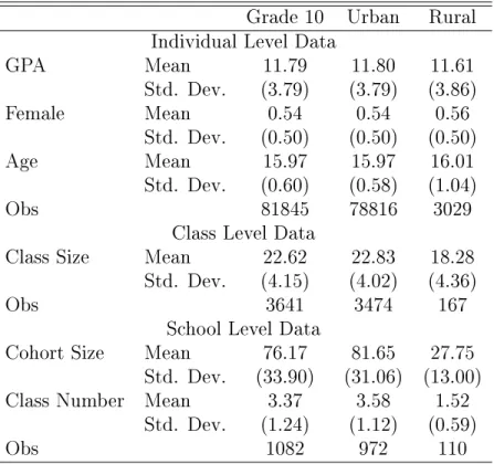
3.1 Summary Statistics

Table 1: Sample means and standard deviations

Grade 10 Urban Rural

Individual Level Data

GPA Mean 11.79 11.80 11.61 Std. Dev. (3.79) (3.79) (3.86) Female Mean 0.54 0.54 0.56 Std. Dev. (0.50) (0.50) (0.50) Age Mean 15.97 15.97 16.01 Std. Dev. (0.60) (0.58) (1.04) Obs 81845 78816 3029

Class Level Data

Class Size Mean 22.62 22.83 18.28

Std. Dev. (4.15) (4.02) (4.36)

Obs 3641 3474 167

School Level Data

Cohort Size Mean 76.17 81.65 27.75

Std. Dev. (33.90) (31.06) (13.00)

Class Number Mean 3.37 3.58 1.52

Std. Dev. (1.24) (1.12) (0.59)

Here we share some patterns in the data that motivate much of what we do below. Table 1 shows the mean and standard deviation for the key variables we use. Note that class size is relatively concentrated around the mean. In fact 90% of the data lies between 16 and 28 class size. The average school has 3 or 4 classes in a grade, but there is a lot of variability here. Rural areas usually have small schools with lower enrollments and number of classes that range from 1 to 3, while urban areas have larger schools with as many as 9 classes.

3.2 Data Patterns

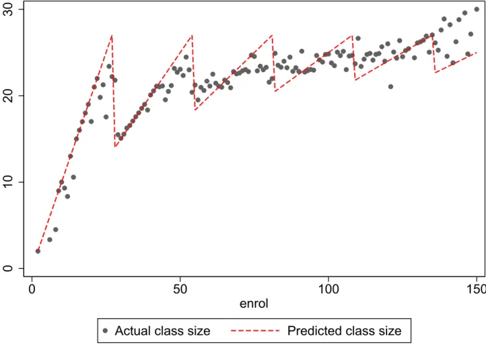
3.2.1 Class Size and Enrollment

Figure 1 plots class size versus enrollment for grade 10. The red dashed line gives the predicted class size had there been a binding cap on class size of 27. The data loosely follows this red line, but since no cap on class size was in place ocially, this targeted class size may be a result of administrators choices. For example, if administrators are trying to maximize some increasing function of learning (as measured by GPA) less costs, given student quality, and nd it roughly optimal to have a class size close to 27, we might see such a pattern.

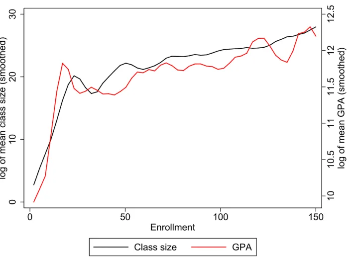
3.2.2 Class Size, Enrollment and GPA

Figure 2 plots a smooth version of the relationship between enrollment and class size given by the black line, and between enrollment and GPA given by the red line. It is worth noting that especially for low enrollments, class size and GPA seem to be negatively related. As enrollment rises, class size rst rises till enrollment reaches the mid 20's. After this class size falls and then rises again near 45 and so on. The turning points of the two seem to be the same. The relationship becomes much fuzzier for large enrollments.

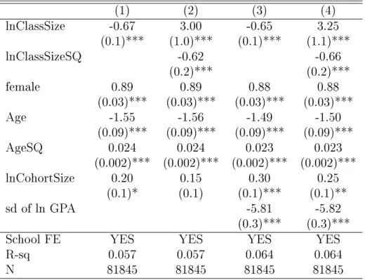
3.2.3 OLS Estimates

As a purely descriptive exercise, we next turn to the OLS estimates of class size and GPA. As is well understood, OLS estimates are likely to be biased and should not be interpreted as causal. Nevertheless, this is the logical starting point for the analysis. Table 2 presents these estimates. Column 1 does not allow for nonmonotonicity and gives a negative and signicant coecient for class size. Column 2 adds a quadratic term in class size. The coecients now point to a hump shape with a turning point around 11. Should we interpret these estimates as representing the production technology in the classroom between class size and GPA or learning? The answer is no.

0 10 20 30 0 50 100 150 enrol

Actual class size Predicted class size Figure 1: Class Size versus Enrollment for Grade 10

10 10.5 11 11.5 12 12.5

log of mean GPA (smoothed)

0

10

20

30

log of mean class size (smoothed)

0 50 100 150

Enrollment

Class size GPA

Table 2: OLS Estimation of Class Size Eects (1) (2) (3) (4) lnClassSize -0.67 3.00 -0.65 3.25 (0.1)*** (1.0)*** (0.1)*** (1.1)*** lnClassSizeSQ -0.62 -0.66 (0.2)*** (0.2)*** female 0.89 0.89 0.88 0.88 (0.03)*** (0.03)*** (0.03)*** (0.03)*** Age -1.55 -1.56 -1.49 -1.50 (0.09)*** (0.09)*** (0.09)*** (0.09)*** AgeSQ 0.024 0.024 0.023 0.023 (0.002)*** (0.002)*** (0.002)*** (0.002)*** lnCohortSize 0.20 0.15 0.30 0.25 (0.1)* (0.1) (0.1)*** (0.1)** sd of ln GPA -5.81 -5.82 (0.3)*** (0.3)***

School FE YES YES YES YES

R-sq 0.057 0.057 0.064 0.064

N 81845 81845 81845 81845

(1)_{Standard deviations are clustered at class level. *, **, *** indicate}

signicance at the 10%, 5%, and 1% levels, respectively.

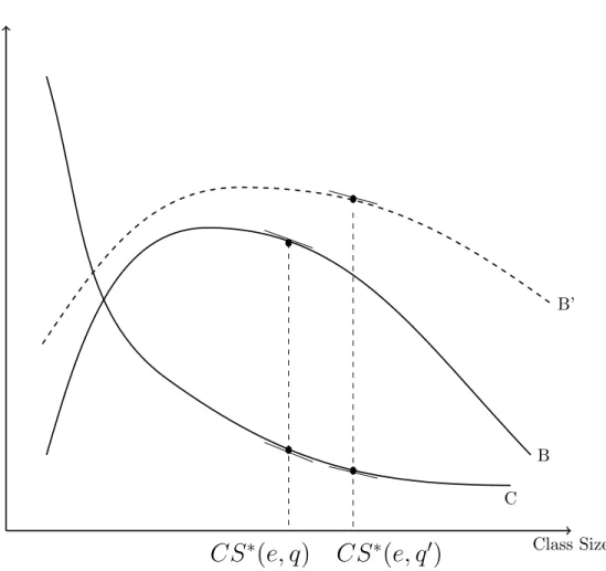
Why? Suppose class size is being chosen to maximize an increasing function of the learning, i.e., the GPA of the school, less costs of operation, and say enrollment is exogenously given. For a given quality of students, or teacher, denoted by q and given enrollment,e, Figure 3depicts the

benets (B) and costs (C) as class size rises. As class size rises, the benets may rst rise but

ultimately fall and this is depicted as concave function.9 _{However, as class size rises, costs fall}

and this is depicted as a downward sloping convex function. Optimal class size, i.e., the chosen class size, is where the dierences in the two is largest. This occurs at CS∗_{(e, q). Thus, in the}

data we will see (e, CS∗_{(e, q), gpa(e, q, CS}∗_{(e, q)). Moreover, we will most likely not observe q.}

What happens if q is higher? If for example, students are better, then the benet curve will

shift up and become atter as depicted by the curve B0 _{since better students would learn more}

(have a higher GPA) at any given class size and suer less from larger classes. But faced with a better class, the chosen class size will rise as depicted to CS∗_{(e, q}0_{) and in the data we will see}

(e, CS∗_{(e, q}0_{), gpa(e, q, CS}∗_{(e, q}0_{)). Though we want to estimate the curve B, the data will trace}

out a atter curve than B. This is the essence of the bias in the OLS estimates and the upward

bias explains why OLS coecients on class size often turn out to be positive.

Class Size B, C B B’ C

CS

(

e, q

)

CS

(

e, q

)

4 Nonparametric Evidence

Recent work by Chernozhukov et al. (2013) provides a framework applicable to our setting and with the advantage that minimal assumptions are needed to estimate the eect of class size on GPA. The approach needs panel data, which we have, and the endogenous regressor (class size) has to be discrete.

Following their approach we specify the following model:

GP Ajt =g(CSjt,αj, εjt)

which has achievement as measured by the average GPA of school j in period t being a function

of the average class size in school j in period t, a school xed eect, αj, and a shock, εjt, that is

school and time specic. This model does not impose any functional restrictions on the relationship between class size and grade point average. Though class size is discrete, average class size is a continuous variable. For this reason we discretize the class size into bins below.

We specify this relationship to be at the school level, because nonparametric estimation of this kind needs a long panel for each j.10

4.1 Assumptions and Approach

The identifying assumption needed for this approach is the following: Assumption 1 (time-homogeneity)

εjt |CSj, αj ∼F(.|CSj,αj).

In other words, the distribution of the shock εjt, conditional on the vector of average class sizes

for the school at all periods (denoted by CSj) and the school itself, is time independent as the

function F has no time subscript. Stated slightly dierently, whatever the distribution of the

shock is, its conditional distribution given the vector of average class sizes for school j does not

depend on t. Chernozhukov et al.(2013) interprets this as time being randomly assigned or time

being an instrument along with the distribution of factors other than class size not changing over time.

10_{If we had specied the model to hold at the individual level, we would have a panel of length three, though}

we would have a lot of students. Similarly, we could have specied the model to be at the class level if we had information on which teacher was assigned to which class. In this case, we would have a panel of the same length as that for the model we use, assuming the teacher was there throughout. We do not have data on teachers and their assignment to classes we cannot use this approach.

Note the contrast to the standard assumptions for the linear model

GP Ajt =βlnCSjt+αj +εjt

where the identifying assumption is that E(lnCSjt ·εjs) = 0 for all t and s. Of course, this

assumption is likely to be violated as class size is highly endogenous. The approach we take does not need this assumption. The distribution that the shock is drawn from does depend on class size. However, it is enough for identication that the shock to be drawn from the same distribution at all times. In eect, variations in class size over time helps identify the eect of interest. Moreover, the specication we use is not restricted in any parametric way and need not even be monotonic. Since the class size is bounded by the cohort size, the class size support is nite. Under Assumption 1, Chernozhukov et al. (2013) show that the average class size eect for schools that switch from class size level a to class size level b (the movers) is identied. As they explain it, to

see this more easily, assume that we have only two class sizes: CSjt ∈ {0,1}. Then the model

can be thought as a treatment eect model where CSjt = 1 for the treated and CSjt = 0 for

the untreated. Denote GP Ajt(0) = g(0, αj, εjt), and GP Ajt(1) = g(1, αj, εjt). Assumption 1

implies that the conditional distribution of (GP Ajt(0), GP Ajt(1)), given the vector of class sizes

for school i(CSj) does not vary with t. Under this key assumption, the average treatment eect

(ATE) for schools where both groups of class size occur during the observation period is identied. This is similar to the local average treatment eect (LATE), which is the treatment eect for the subpopulation that changes its treatment status due to a change in the instrument. As explained above, time is like an instrument. Thus, the eect of class size on grade point average for schools that ever changed their class size at some time is identied.

One might be concerned that Assumption 1 does not hold in the data and as a result, the approach of Chernozhukov et al. (2013) cannot be used. Fortunately, we need not take the as-sumption on faith. A recent paper, see Ghanem (2017) derives a statistical test to check the validity of Assumption 1. In the Appendix A we show that using this methodology, we cannot reject the hypothesis that Assumption 1 holds in the data.11

4.2 Estimates

We choose to discretize class size into three bins. We do so as we will need to estimate the eect going from each bin to the other so that the number of coecients rises rapidly with the number of bins. The rst is class size below a cuto s0. The second bin is from s0 to s1, and the third is

more than s1. Since these switches are identifying the eects of interest, we need to chooses0 and

s1 to ensure that the bins are such that these switches occur.

Letδlk be the average eect on mean GPA in a school of switching from binl tok and δˆlk be

its consistent estimator. In eect, what is done is the following. In each year, each school has a mean GPA and a mean class size and so falls into one of the three bins. Over the entire sample period, each school indexed by j can be in either bin 1 only, bin 1 and 2 only, bin 1 and 3 only,

bin 2and 3 only or in all three bins. We calculate the mean GPA over time for school j when in

bin l = 1,2,3. For example, if there were 5 periods and the school was in bins (1,2,1,3,2) over

these time periods with GPA (g1, g2, g3, g4, g5), then the mean GPA in bin 2 would be (g2+g5)/2

while the mean GPA in bin1 would be(g1+g3)/2.Their dierence would capture∆j12for school

j. The estimated ˆδ12 would then be

ˆ δ12= N P j=1 dj∆j12 N P j=1 dj

where dj is 1 if the school was ever in both bin 1 and 2over the entire sample period.

We set s0 at 15 and s1 at 22. ˆδ12 = 1.55 and δˆ23 =−.18. Both are signicantly dierent from

zero at the 1% level. In Table A.1 in the Appendix B, we vary s1 from 21 to 24 along the rows

and s0 from 12 to 17along the columns. For each value of s0 and s1 we give the estimate of δˆ12

and _δˆ_{23. Note that no matter what s0 to s1 are set at, δ}ˆ_{12 > 0,δ}ˆ_{23 < 0 and signicant. This is}

consistent with a nonmonotonic relationship between GPA and class size.

5 Linear and Nonlinear Parametric Estimates

In view of the nonparametric results above which suggest an inverseU shape for the eect of class

size on GPA, we include a quadratic term in the parametric specication. Our specication is:

GP Aijt=βlnCSjt+γ(lnCSjt)

2

+αj +λXijt+εijt.

GPA for individual i in school j at time t depends on the log of class size, its square, school xed

eects, and a set of control, Xijt, which include gender, age, age squared, the standard deviation

of the GPA in the class. Why might class size and GPA be hump shaped? One reason given in the literature, see Borland et al. (2005) and Dobbelsteen et al. (2002), is that students learn from peers like themselves. The larger the class size, the more likely it is that they have peers like themselves. This force makes GPA rise with class size. On the other hand, a larger class

size reduces the attention a teacher can give to each student. For low class sizes, the rst set of forces dominate but after a point the second does, creating a hump shaped pattern. It has also been argued that a homogeneous class is easier to teach, see Levin (2001) and Dobbelsteen et al.

(2002). For this reason we include the standard deviation of GPA in the class as a control. Since class size could be an endogenous variable, we need an instrument. We cannot use the

Angrist and Lavy(1999) approach. There is no maximum class size on the books in Greece in our

period. The data patterns described in Section 3.2 clearly suggest that class size is endogenous. From looking at the pattern of enrollment and class size in Figure 1, it seems clear that class size is not allowed to get too large: the actual and predicted class size had there been a cap of 27 are not quite in line though they are closer together for low enrollment than for high.12 _{We follow}

the approach of Hoxby (2000). It is natural to think of overall enrollment as an exogenous shock to class size. Hoxby's approach goes a step further: she ts a quartic to the enrollment data and uses deviations from the quartic as the exogenous variation. In this way, she controls for trends in enrollment.

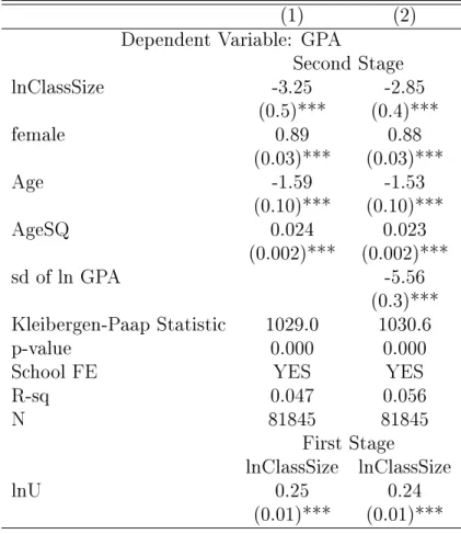
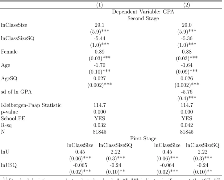
Table 3 and Table 4 give the IV estimates for grade 10 for the linear and quadratic models respectively. We present estimates when the standard deviation of GP Ain the class is controlled

for and when it is not. The standard errors are clustered at the class level. The lower panel of the table gives estimates for the rst stage while the upper panel gives the estimates for the second stage in all these tables.

Recall that the OLS estimate of the coecient on lnClassSize in the linear regression was

negative and about -.067. The coecient with the IV for the same regression is given in column 1 and is -3.25. Note that this is exactly what one would have expected due to endogeneity bias. If the administrator is choosing class size, classes with better students will tend to be larger as such larger class size has little cost in terms of GPA and OLS is upward biased as in these estimates. If we add the standard deviation of GPA as a control, as in column 2, the coecient on lnclass size is slightly smaller. The coecient on standard deviation is negative, consistent with more diverse students being harder to teach. Table4gives the estimates for the quadratic specication. It clearly has the hump shape expected with a peak at around 14.9.

We use Hoxby's instrument so that we would expect the shock in enrollment to be positively correlated with class size as we nd. Note that the rst stage looks ne: the coecient on the instrument is positive signicant at 1% and the instruments are not weak as the Kleibergen-Paap LM statistic is 114.7. It is interesting, and in line with the literature that women have a higher GPA. The standard deviation of GPA in a class is added as an explanatory variable in the second

12_{In fact, when we tried using the Angrist Lavy approach, though the rst stage did not cause any problems, the}

column of Table 3 and Table4. It is signicant at the 1% level and negative. This suggests that the more homogeneous the class, the higher the GPA as in Levin (2001) and Dobbelsteen et al.

(2002).

While we nd strong evidence for a nonmonotonic relationship between class size and achieve-ment, our results are entirely consistent with ndings in the literature, see for exampleJepsen and

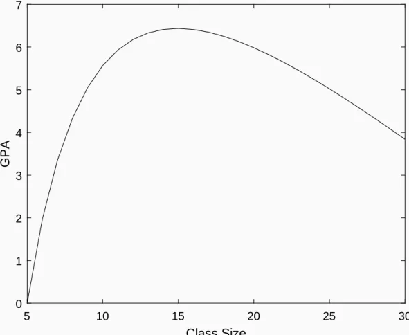
Rivkin (2009), that reducing class size is an expensive way of improving achievement. Figure 4

depicts the quadratic relation we estimate. Note that the value of the intercept is not meaningful as we have school xed eects and other controls. We choose to center the gure at class size 5 and GPA zero. The curve is relatively at in the region near the peak by denition. As a result, changing the class size in this region would give small eects. If the curve is not too peaked, this region could be quite large. This might be why even the experimental literature, see Jepsen and

Rivkin (2009) for example, found small eects on performance of fairly large changes in class size.

Table 3: Parametric Estimation of Linear Class Size with IVs

(1) (2)

Dependent Variable: GPA

Second Stage lnClassSize -3.25 -2.85 (0.5)*** (0.4)*** female 0.89 0.88 (0.03)*** (0.03)*** Age -1.59 -1.53 (0.10)*** (0.10)*** AgeSQ 0.024 0.023 (0.002)*** (0.002)*** sd of ln GPA -5.56 (0.3)*** Kleibergen-Paap Statistic 1029.0 1030.6 p-value 0.000 0.000

School FE YES YES

R-sq 0.047 0.056 N 81845 81845 First Stage lnClassSize lnClassSize lnU 0.25 0.24 (0.01)*** (0.01)***

(1)_{Standard deviations are clustered at class level. *, **,}

*** indicate signicance at the 10%, 5%, and 1% levels, respectively.

Table 4: Parametric Estimation of Nonlinear Class Size with IVs

(1) (2)

Dependent Variable: GPA Second Stage lnClassSize 29.1 29.0 (5.9)*** (5.9)*** lnClassSizeSQ -5.44 -5.36 (1.0)*** (1.0)*** Female 0.89 0.88 (0.03)*** (0.03)*** Age -1.70 -1.64 (0.10)*** (0.09)*** AgeSQ 0.027 0.026 (0.002)*** (0.002)*** sd of ln GPA -5.76 (0.4)*** Kleibergen-Paap Statistic 114.7 114.7 p-value 0.000 0.000

School FE YES YES

R-sq 0.032 0.042

N 81845 81845

First Stage

lnClassSize lnClassSizeSQ lnClassSize lnClassSizeSQ

lnU 0.45 2.22 0.45 2.22

(0.06)*** (0.3)*** (0.06)*** (0.3)***

lnUSQ -0.065 -0.24 -0.064 -0.24

(0.02)*** (0.10)** (0.02)*** (0.10)**

(1)_{Standard deviations are clustered at class level. *, **, *** indicate signicance at the 10%, 5%,}

and 1% levels, respectively.

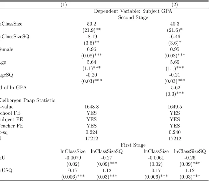
A possible concern might be that we have so far not controlled for which teachers taught which class. We were able to obtain and digitalize teachers' assignment data for 10 schools. For this subsample, we are able to control for teacher xed eects as a robustness check, to control for the teachers' quality. The dependent variable is GPA for each subject and for each student, not the average GPA since we are controlling for teacher xed eects. In addition to teachers' xed eects, we include subject and school xed eects in Table 5. Though the point estimates do change a bit, the quadratic form remains. For the rest of the paper, we return to using the full sample.

Table 5: Nonlinear Class Size with Teachers' Fixed Eects

(1) (2)

Dependent Variable: Subject GPA Second Stage lnClassSize 50.2 40.3 (21.9)** (21.6)* lnClassSizeSQ -8.19 -6.46 (3.6)** (3.6)* Female 0.96 0.95 (0.08)*** (0.08)*** Age 5.64 5.69 (1.1)*** (1.1)*** AgeSQ -0.20 -0.21 (0.03)*** (0.03)*** sd of ln GPA -5.62 (0.3)*** Kleibergen-Paap Statistic p-value 1648.8 1649.5

School FE YES YES

Subject FE YES YES

Teacher FE YES YES

R-sq 0.224 0.240

N 17212 17212

First Stage

lnClassSize lnClassSizeSQ lnClassSize lnClassSizeSQ

lnU -0.0079 -0.27 -0.0061 -0.26

(0.02) (0.09)*** (0.02) (0.09)***

lnUSQ 0.17 1.12 0.17 1.12

(0.006)*** (0.03)*** (0.006)*** (0.03)***

5 10 15 20 25 30 Class Size 0 1 2 3 4 5 6 7 GPA

6 Quantile Eects

So far we have allowed for nonmonotonicities in how class size aects GPA. In this section, we extend our approach to allow for quantile eects. We do so as it is possible that students of dierent abilities respond dierently to larger class size. One hypothesis is that better students are less aected by class size as they are able to do it alone. If this were the case, we might expect a hump shape for all quantiles, but with the hump being attened out at higher quantiles. It is worth recalling that a quantile regression does not simply take the data and split it into quantiles, conditional on the independent variable, as doing so would result in selection bias. Rather, it does something more subtle. Suppose we had a linear regression model,

y =Xβ+u

where we observe data(Xi, yi)fori= 1...nindividuals, and we wanted to allow for quantile eects.

Since y−Xβˆwould be the best proxy for u, the coecient βˆα for the linear regression for the

αth quantile is obtained as ˆ βα =arg min X i α_|yi−Xiβ|I(yi−Xiβ >0) + (1−α)|yi−Xiβ|I(yi−Xiβ <0).

Supposeα=.1. Then, for individualithere is a 10%probability that yi−Xiβ >0and a90%

probability that it is negative. The above formula chooses _βˆ_{.1 so that if 10% of the deviations are}

positive and 90% are negative, the expected deviations are minimized. Note the contrast to the

simple minded approach described above. In fact, even if the model were truly linear, choosing

10% of the data at any X to lie below the estimated regression would not even give a linear

regression coecient.

We use the approach of Lee (2007) to estimate the quantile IV regressions. Note that we do not include school xed eects in the quantile IV regression since we were unable to include such a large number of xed eects. We use the same instrument as in the previous section. We present the quadratic version of the regression.

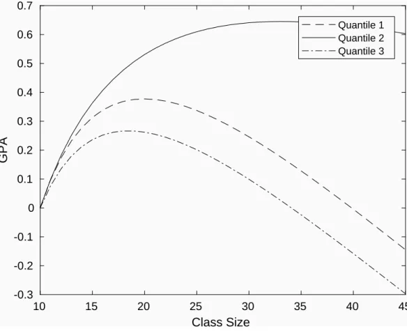
Table 6gives the estimates for the quadratic form and Figure5depicts these estimates graph-ically. Note that in order to be able to compare the three curves visually we anchor them to zero at class size 10. It is worth noting that the hump shape remains. However, it is clear from this depiction that the 10% quantile (the worst students) is more hump shaped than the 50% quantile which in turn is slightly more hump shaped than the 90% quantile. This is exactly what one would expect if better students are less aected by class size.

While we have specied a quadratic form for our model which allows for nonmonotonic rela-tionship between GPA and class size in our quantile regressions, it would be ideal to do this fully nonparametrically. Unfortunately, we are unaware of any technique to do so at this time and this is left for future work. Note that we did estimate the regression, though not allowing for quantile eects, nonparametrically in Section 4.

Table 6: Quantile Regressions

(1) (2) (3)

Quantile 10% Quantile 50% Quantile 90%

lnClassSize 4.73 3.15 4.14

[3.80,6.41] [1.79,5.72] [1.04,5.85]

lnClassSizeSQ -0.79 -0.45 -0.71

[-1.07,-0.62] [-0.89,-0.19] [-0.99,-0.20]

(1)_{The brackets are the 95% condence intervals.}

10 15 20 25 30 35 40 45 Class Size -0.3 -0.2 -0.1 0 0.1 0.2 0.3 0.4 0.5 0.6 0.7 GPA Quantile 1 Quantile 2 Quantile 3

Figure 5: Quantile Eects of Class Size (Three quantiles)

With the estimates of the eects of class size on achievement in hand, we are in a position to understand how class size might be chosen. If the government cares about achievement, and faces

costs of adding and removing classes, its behavior in terms of the number of classes it chooses as enrollment uctuates helps us estimate the costs involved. We use our reduced form estimates with a dynamic structural model of class size to estimate hiring/ring and marginal cost of adding a class. In Greece, as in much of the rest of the world, teachers unions are a powerful force to be reckoned with. Their power is expressed not only in terms of wages set but in terms of the ability to re teachers at will. We use the model to ask whether inexibility in terms of unions creating high ring (and even maybe hiring) costs might be driving class size choices by government and the impact of this on student achievement if any. We nd that unions, even if they raise costs and class size have a small eect on achievement.

7 The Structural Model

In the previous sections, we have shown that GPA has an inverse U shape with respect to class size. In this section, we ask what an administrator who is trying to do his best for his students but subject to constraints would choose to do. We posit that the administrator is trying to maximize a welfare function that depends on the mean GPA of the students enrolled, as well as the number of students enrolled. Enrollment, et, is taken as an exogenous AR1 process and estimated from

the data.

et=γ0+γ1et−1+µt (1)

where, et is assumed to follow a Poisson distribution with mean γ0 +γ1et−1 with the error term

µt. We estimate the enrollment process separately for schools of dierent sizes. We put roughly

25% in the small and large enrollment groups and 50% in the middle enrollment group.

The constraints the administrator faces are of two kinds. First, he faces the trade o we have estimated between class size and GPA and the enrollment process which is exogenously given to him. We can think of these as technical constraints.13 _{Second, he faces costs associated with the}

choices he makes. In our model, the only choice the administrator makes is the number of classes,

nt, to have at a point of time. Each additional class has a given cost which can be thought of

as the cost of the teachers needed for the additional class. Since teachers unions are prevalent in Greece, ring teachers is costly. Moreover, nding a new teacher also involves a number of costs including advertising the position, interviewing, and so on. The empirical transition probabilities are in Table 7. Note that schools tend to keep the same number of classes across years. This is

13_{The trade-o between GPA and class size the administrator faces is analogous to the production function a}

manager choosing inputs would face. The enrollment process (et) can be thought of as similar to an exogenous

especially so for schools with a small number of classes.

For these reasons we allow for hiring and ring costs in the model. This makes the problem dynamic. At any point of time, the administrator must consider the number of teachers he has, the enrollment today and the enrollment process he faces, as well as the range of costs and look forward to nd his best decision today.

Table 7: Transition of Class Number

nt−1 nt _{1 2 3 4 5 6 7} 1 0.7143 0.2727 0.0130 0.0000 0.0000 0.0000 0.0000 2 0.0813 0.6986 0.2010 0.0144 0.0048 0.0000 0.0000 3 0.0034 0.1399 0.6007 0.2389 0.0171 0.0000 0.0000 4 0.0000 0.0036 0.2456 0.5979 0.1459 0.0071 0.0000 5 0.0000 0.0000 0.0405 0.2162 0.6622 0.0743 0.0068 6 0.0000 0.0000 0.0000 0.0645 0.3871 0.4194 0.1290 7 0.0000 0.0000 0.0000 0.0000 0.0000 0.7500 0.2500

The administrator cares about the mean GPA. As this has a quadratic form, and as e

n is the

average class size, we have

GP At=aln et nt +b lnet nt 2 +A.

A is the value of the other variables in the regression at their mean levels. It is worth noting that

its value will not aect the choice of the number of classes below. We assume that having twice the students with the same GPA gives the administrator twice the utility. This makes sense as the object is to educate students and educating twice as many to the same level gives twice the utility. Thus, so far we have the administrator's utility as

et " aln et nt +b ln et nt 2 +A # .

The administrator faces hiring and ring cost of H and F, and a variable cost per class of c which we interpret as the salary of the additional teacher(s) needed for one more class. The

administrator knows the realization of et and knows the state variable, nt−1, and the random

utility shock εnt, when he makes his choices. This shock is not observed by the econometrician. εt={ε1t, ε2t, ε3t...ε10t}is a vector of shocks and each element is drawn from a type 1 generalized

extreme value distribution. Since no school has more than 10 classes, we restrict the size of the

vector to be 10. This assumption allows us to use the logit setup and t the data parsimoniously.

this comes partly from enrollment declines, partly because fewer classes were present in the past and there are hiring costs, and partly from the shock.

Thus, the administrators value function is:

V(et, nt−1,εt;θ) = M ax nt ( et " aln et nt +b ln et nt 2 +A # −cnt −H_·max(nt−nt−1,0)−F ·max(nt−1−nt,0) +εntt +δEεt+1,et+1V(et+1,nt,εt+1;θ) )

whereet+1 = γ0+γ1et+µt+1 and whereθ = (c, H, F, σ).

Note that the expectation is taken over both εt+1 and et+1, the shock to utility and the shock to

enrollment respectively. Note that though Aet enters the objective function, it will not aect the

optimal choice of nt as it is exogenous. From here on we may not explicitly condition on θ as

above, but it should be taken for granted.

Rewriting this slightly for notational ease we dene u(et, nt, nt−1) as the deterministic

com-ponent of current period contribution to the objective function and V(et, nt−1) as the ex ante

value function, i.e., the value of behaving optimally from tomorrow onwards before knowing the realization of the utility shock.

u(et, nt, nt−1) = et " alnet nt +b ln et nt 2 +A # −cnt −Hmax(nt−nt−1,0)−F max(nt−1−nt,0) V(et+1, nt) = Eεt+1[V(et+1, nt,εt+1)] v(et, nt, nt−1) = u(et, nt, nt−1) +δEµt+1[V(et+1, nt)|et] (2) so that V(et, nt−1, εt) = max nt v(et, nt, nt−1) +εntt.

Thus we have rewritten the value function as a base utility and a shock. Since εntt follows an

iid type 1 generalized extreme value distribution with variance σ2_{, the probability of n}

t is p(nt|nt−1, et;θ) = exp(v(et, nt, nt−1;θ)) P10 n=1exp(v(et, n, nt−1;θ)) .

7.1 Identication and Estimation

We rst provide some intuition behind what pins down θ before we turn to the estimation part.

The problem is modeled as a dynamic discrete choice problem. We bring the estimates of the quadratic model for achievement from the reduced form regressions to the structural model. As estimated in the parametric quadratic model, b = −5.36 and a = 29.0. It remains to estimate θ = (c, H, F, σ). How can we identify θ? One way to get some intuition about which features of

the data would help identify which parameters is to ask how a simulation based approach might pin down the parameters. We do not use this approach, but nevertheless, this is a useful exercise. To see how the optimization works, it is useful to think of the problem in a slightly dierent way where we rst dene the pre-value function as W(et, nt, εntt). W(.) is the value of the ow

utility today (excluding the adjustment costs) and behaving optimally from tomorrow onwards for every value of nt chosen today. Note that we have a choice in terms of the parameters to

estimate: the weight on GPA or the variance of the utility shock since both cannot be separately identied. We choose to set the weight on GPA at unity as the variance of the utility shock is easier to interpret. W(et, nt, εt) = et " aln et nt +b lnet nt 2# −cnt+εntt +δEεt+1,µt+1V(et+1,nt,εt+1) (3) Then, V(et, nt−1, εt) = max nt { W(et, nt,εt)−H·max(nt−nt−1,0)−F ·max(nt−1−nt,0)}

To begin with, let us see how the model works when we taken to be continuous, the pre-value

function to be concave, and set the utility shocks to zero. In this case, the current period problem can be depicted as in Figure 6where W(et, nt,εt= 0) is depicted by the concave curve. Consider

such a school with a given enrollment as well as utility shocks set at zero. Anchor the linear adjustment costs to nt−1 as depicted. The cost of increasing the number of classes has slope H

and decreasing it has slope F while making no change in their number has no cost. The optimal

choice ofntis that which maximizes the dierence in the pre-value function and these adjustment

costs. Let nL _{be where the slope of the pre-value function is H and n}H _{be where the slope is}

−F. It is obvious from the picture that if nt−1 exceeds nH, it is optimal to reducent to nH, i.e.,

increase class size, and if nt−1 falls short of nL,to raise nt−1 to nL, that is reduce class size. If

nt−1 lies in the interval

nL_{, n}H

by these adjustment costs which are not dierentiated at 0. The higher the adjustment costs, the larger this region of inactionue.14 _{The size of H and F will be pinned down by the bounds of the}

region of inaction,

nL_{, n}H

which would be observed in the data.15

Class Number

W

(

·

) Adjustment Cost

W

(

·

)

n

t

₋

1

n

L

n

H

n

t

₋

1

Figure 6: Identication of Adjustment Cost H, F

When we add back the utility shocks and the discreteness of n, the stark predictions of the

restricted model above are tempered. The depiction in Figure 6 changes so that the pre-value

14_{It is worth noting that a change inHorFwill also shift the pre-value function as it will change the continuation}

value. However, this eect will be second order relative to the direct eect of H andF.

15_{It can be shown that the eect of an increase in hiring costs will be greater forn}L_{,the hiring cuto, than for}

nH_{, the ring one. Similarly, an increase inF will have a greater eect forn}H _{than for n}L_{.Thus, if we think of}

the combinations ofH andF that are consistent with a given value for the hiring cuto as well as those consistent

with the ring cuto we will get a unique value of H andF which are consistent with both. As a result, there is a

function is discretized. At each of the ten values taken by n, there is a base value plus the shock.

As a result, the curve connecting the grid points of the analogue of the pre-value function need not be concave. However, the optima choice will still be such that given nt−1, the dierence in

the pre-value and adjustment costs is maximized. And an increase in the adjustment costs would increase the region of inaction and aect the probability of transitioning into this region. In this way, the empirical transition probabilities help pin down H and F in the data.

These same empirical transition probabilities also help pin down the variance of the shock. Given the enrollment process, when the variance rises, the transition probabilities also rise.

How is the nal parameter, c, pinned down? As c rises, having more classes becomes more

expensive and the number of classes falls. Thuscis pinned down by the average number of classes

given enrollment, or equivalently, the average class size.

Having sketched out the intuition behind identication, we move on to the details of estimation. The estimation can be thought of as proceeding in two steps. First estimate the process for enrollment. Then estimate θ.

7.2 Estimating Enrollment

We rst test for whether the AR1 process we specify ts the data. We break the data into three parts. For schools with enrollment less than or equal to 53, for schools with enrollment above 53 but below 99 and for schools with enrollment greater than or equal to 99. Think of these as small schools with one class per grade, medium schools with one or sometimes two classes a grade, and large schools with two or more classes per grade. We then run the AR1 process separately for each of these three groups. Finally we test whether the estimates for the three groups dier from each other. We expect that γ1 might be the same, but thatγ0 is likely to be lower for smaller schools.

Our reason for expecting this is that these schools tend to stay in the same rough size groups, though their enrollment uctuates year by year. The enrollment process is given by equation (1). If there was no random component, µt, then this enrollment process results in the data generated

by it being on the straight line with slope less than 1 depicted in Figure 7. This would result in a steady state at point A in Figure 7. This means that all schools would have the same enrollment

in steady state. Adding a random component will make the process generate data that falls in a band around the straight line in Figure 7. The width of this band depends on the variance of µt.

This will give a distribution of steady states in Figure 7. Note that in this case, schools will not tend to stay in their own rough groups over time.

What would be consistent with schools staying in their own group? If γ0 was dierent (and

Enrollment int Enrollment int+ 1 45◦ Small Medium A Large

Figure 7: Enrollment Process

0 20 40 60 80 Enrollment at t+1 10 20 30 40 50 60 Enrollment at t

the process without a random component would be depicted by the lines in Figure 7. Note that as depicted, each group has a dierent steady state size interval. Adding back randomness would create bands around the lines as before and create a distribution of steady states for each group size, as shown in Figure 8. If these intervals overlapped, there could be some movement between groups in steady state. The estimates for the estimated enrollment process from the actual data for each group are presented in Table 8. Figure 9 depicts both the actual data and the estimated lines. Note that the actual data and lines look a lot like the simulated data. In particular, the slopes are not signicantly dierent from one another while the intercepts dier signicantly from each other.

Table 8: Estimation of Enrollment Process

<= 53 53< enrol <99 >= 99 γ1 0.71 0.60 0.63 sd (0.01) (0.01) (0.02) γ0 10.27 30.45 43.08 sd (0.49) (0.94) (2.42) N 264 535 244

(1)_{The standard errors are presented in}

parentheses. 0 50 100 150 200 Enrollment at t+1 0 50 100 150 200 Enrollment at t

7.3 Estimation of

θ

Recall that since εt is assumed to have an iid type I generalized extreme value distribution, we

know that equation (4) holds.

p(nt|nt−1, et,θ) = exp(v(et, nt, nt−1)) P10 n=1exp(v(et, n, nt−1)) . (4) V(et, nt−1) = Eεtmax nt [v(et, nt,nt−1) +εntt] = 10 X nt=1 p(nt|nt−1, et,θ)Eεt(v(et, nt,nt−1) +εntt|nt is optimal) since Eεtmax n f(n, εt) = P n

p(n)Eεt[f(n,εt|n being the maximum] where p(n) is the probability

that n is the maximum at a particular value. In other words, the ex-ante value function is just

the probability that each is the optimal choice (given enrollment today and the number of classes inherited) times the payo from then on.

Using the form of the distribution of εt and some calculations yields

V(et, nt−1) = ln 10 X n=1 exp u(et, n, nt−1) +δEet+1[V(et+1, n)|et] ! +γ

where γ is Euler's constant.

By value function iteration, we can solve V(e, n), and thus v(et, nt−1, nt). This is essentially

nding a xed point of a function. By taking a grid and guessing values of the function V(et+1, n)

over the grid, this reduces the problem to a nite dimensional one. eis allowed to take values from 1 to1000 since the largest school in the data has far less than1000 students. This guess, together

with the estimated process for enrollment gives a numerical value of Eµt+1[V(et+1, n)|et] over the

grid. For given parameter values, we can calculate u(et, n, nt−1) so that we get a numerical value

for the RHS over the grid which is the new guess. We stop when the guess and the new guess are close enough, i.e., when we have a xed point. Since δ < 1 and the enrollment process is stable,

i.e., γ1 <1, this is a contraction mapping and this process converges to the xed point. Having

solved for V(et+1, n) we use equation (2) to solve for v(et, nt, nt−1), which in turn gives the value

for p(nt|nt−1, et;θ). Finally, we choose θ to maximize the likelihood of the empirical transition

probabilities

to get the estimated θ.

Table 9: Estimation of the Structural Dynamic Model

Average Cohort Size c H F σ

All 171.30 99.06 156.49 140.24

sd (51.59) (42.90) (42.41) (19.82)

Euro e20,572 e11,896 e18,793

The estimates are presented in Table 9. A larger variance indicates that idiosyncratic shocks matter more when schools choose the number of classes. Idiosyncratic shocks could be the avail-ability of spaces and teachers. The variable cost of adding a class is given by c. The xed cost of

adding a class is H while the xed cost of subtracting a class is F.

Suppose that the cost of an additional class is one teacher's salary in Greece. The salary after 15 years' experience with minimum training for a high school teacher is about e20,572 in 2004

(Stylianidou et al., 2004). H and F are the adjustment costs per class. To get the adjustment

cost in Euros, we divide H byc and then multiply by the Euro cost of an additional class. These

Euro cost estimates are given in the lower part of the entry in Table 9. It costs e11,896 to add a new class and e18,793 to drop a class. The cost of dropping a class is much higher than the cost of adding a class. This is reasonable in Greece as ring a teacher is hard for public schools. The optimal class size in the absence of adjustment costs is 27.

7.4 Counterfactual Exercises

In Greece, as in many countries, teachers are unionized and as a result, ring a teacher is quite costly. The rst counterfactual exercise we consider is the eect of reducing ring cost to zero. How would this aect the class size and GPA. On the one hand, ring teachers will be easy which will raise class size relative to the status quo. This is the direct eect. On the other hand, since its easy to re teachers, it is more likely they will be hired, which reduces class size. This is the indirect eect. Ex ante, the net eect is not obvious. The results of this counterfactual are presented in Table 10. We use the estimated processes for enrollment for each size school to simulate the model. We simulate 1000 schools for each school size. For each simulated school, we simulate 100 periods. We calculate the mean eects using the last 10 periods as the data is by then invariant to choice of starting point. The simulations show that class size and GPA change for the dierent school groups as in Table 10. Reducing ring cost to zero raises average class size by about 4 students and reduces GPA by about a point (recall the scale was from 1-20) and by more for smaller schools than for larger schools. Since class size is larger, fewer teachers are