April 2011, Volume 40, Issue 10. http://www.jstatsoft.org/
spa
: Semi-Supervised Semi-Parametric
Graph-Based Estimation in
R
Mark Culp
West Virginia University
Abstract
In this paper, we present an R package that combines feature-based (X) data and graph-based (G) data for prediction of the response Y. In this particular case, Y is ob-served for a subset of the observations (labeled) and missing for the remainder (unlabeled). We examine an approach for fitting ˆY =Xβˆ+ ˆf(G) where ˆβ is a coefficient vector and
ˆ
f is a function over the vertices of the graph. The procedure is semi-supervised in na-ture (trained on the labeled and unlabeled sets), requiring iterative algorithms for fitting this estimate. The package provides several key functions for fitting and evaluating an estimator of this type. The package is illustrated on a text analysis data set, where the observations are text documents (papers), the response is the category of paper (either applied or theoretical statistics), the X information is the name of the journal in which the paper resides, and the graph is a co-citation network, with each vertex an observation and each edge the number of times that the two papers cite a common paper. An appli-cation involving classifiappli-cation of protein loappli-cation using a protein interaction graph and an application involving classification on a manifold with part of the feature data converted to a graph are also presented.
Keywords: semi-supervised learning, graph-based classification, semi-parametric models,R.
1. Introduction
In this work, we present a package geared towards providing a semi-supervised framework for processing semi-parametric models. In this setting, the data are partitioned into two sets, one is a feature setX and the other is either an additional feature set Z or observed graph
G. Here X is an n×p data matrix, Z is ann×q data matrix, and the observed graph G
can be written asG= (V, E), where the nodes inV correspond to the observations and E is the set of similarity edges between observations. We have a labeled response for a subset of the observations, denoted byYLof lengthm≤n. The data matrixXcan be partitioned into
X= [XL>, XU>], such thatXL> corresponds to the cases for which the response is labeled. The response is missing (unlabeled) for the cases in XU>, and we denote these missing values as
YU. An analogous partition can be made for an additional data matrixZ. For the observed graphG, the adjacency matrix can be partitioned as follows,
A= ALL ALU AU L AU U ,
where ALL are the labeled-labeled edges, AU L = A>LU are the labeled-unlabeled edges, and
AU U are the unlabeled-unlabeled edges. For these data we assume that theE[Y] =Xβ+f(G) for some true β and f. The objective is to use all of the data, including those cases with a missing response, in conjunction with the labeled responsesYL to obtain an estimator of the formXβˆ+ ˆf(G).
There are several approaches in existence to perform the difficult task of semi-supervised classi-fication with graphs, including mini-cut algorithms (Blum and Chawla 2001;Kondor and Laf-ferty 2002), directed graph algorithms (Eppstein, Patterson, and Yao 1997;Zhou, Sch¨olkopf, and Hofmann 2005), graph regularization algorithms (Belkin, Matveeva, and Niyogi 2004;
Joachims 2003;Zhu, Ghahramani, and Lafferty 2003), and graph smoothers (Culp and Michai-lidis 2008a;Nui, Ji, and Tan 2005;Wang and Zhang 2006). The natural approach to do this is loss function optimization via regularization, where here the smoothness of the function is controlled with respect to the discrete combinatorial Laplacian operator on the graph (Zhu 2008). The problem of combining X information with a graph G (either observed or con-structed from Z) is often referred to as graph-based co-training (Joachims 2003; Culp and Michailidis 2008a). Existing semi-supervised graph-based approaches for the objective re-quire one to first convert theZ data to a graph, Z →G[Z] and then setGF =G[Z]∪G, or
GF =G[Z]∩G(Culp and Michailidis 2008a). The next step is to employ one of the above graph-based semi-supervised classification approaches directly toGF. The proposed approach implements both the fitting the fits algorithm (FTF) in (Culp and Michailidis 2008b) and the more general sequential predictions algorithm (SPA) (Culp and Michailidis 2008a), both of which perform graph-based classification with the additional flexibility of processing the X
data on its original scale. This is most desirable forX data that are not continuous. The semi-supervisedspapackage is designed to fit ˆY =φsuch that the form of φis:
φ(X, G) =Xβˆ+ ˆf(G)
where ˆf is a function over the vertices ofG and ˆβ isp×1 coefficient vector. The challenges for this approach include simultaneous semi-supervised estimation of a coefficient vector and a function over the vertices of G. Applications for an estimate of this form occur in text analysis, where the observations in the data are published text documents and the response is the document’s topic. In this case a graph describing pairwise co-citations between documents is observed directly (the edge weight is the number of times that two papers reference the same documents). In addition the journal in which the document was published is available as feature informationX. Therefore, we would wish to estimate φ=Xβˆ+ ˆf(G) to combine these two sources of information for classification. Several other applications of this research are quite common in web analysis (Blum and Mitchell 1998), email (Koprinska, Poon, Clark, and Chan 2007), proteomics (Kui, Zhang, Mehta, Chen, and Sun 2002;Ruepp, Zollner, Maier, Albermann, Hani, Mokrejs, Tetko, Guldener, Mannhaupt, Munsterkotter, and Mewes 2004),
genomics and drug discovery. In addition to observed graphs, this work is also applicable as an extension of standard semi-parametric modeling, where an additional feature set Z is observed separately from X. In the classical semi-parametric setting one would commonly fit φ(XL, ZL) = XLβˆ+ ˆf(ZL) where f is a smooth function. For the spa package in this case we provide severalRfunctions to convert Z to a proximity graph, Z → G[Z] and then subsequently fitφ(X, G[Z]) = Xβˆ+f(G[Z]). The advantage is that the information in XU andZU influence training ofφ, that is, the estimates are semi-supervised.
The spa package is written for theRprogramming environment (RDevelopment Core Team 2011) and available from the ComprehensiveRArchive Network athttp://CRAN.R-project. org/package=spa. This package provides the implementation of the sequential predictions al-gorithm. The package design consists of three general phases: (i) graph construction, (ii) con-structing the spa object and (iii) post fitting functionality. The graph construction segment provides a series of functions to process observed graphs or to construct graphs from part of the feature data. Upon completing this stage ann×nadjacency matrix is obtained with diagonal elements representing nodes (observations in the data) and off-diagonal elements representing edge associations between nodes. For the second phase a SPA object is created from the inputs using semi-supervised smoothers (discussed in Section 3). One technical challenge common with smoothers is tuning parameter estimation. The SPA features sophisticated algorithms for data driven estimation of the smoother parameter based on a semi-supervised generalized cross-validation measure. Step (ii) completes with a SPA object that encapsulates φ.
The post fitting step consists of generic function utilities for manipulating and accessing a SPA object, such as coefandfitted, functions toplotandprintthe object, and functions for performing prediction/updating with the SPA object. The prediction/updating function-ality for the package was carefully designed to distinguish betweentransductive andinductive
prediction. Transductive prediction requires re-training or updatingφto use local proximity information with the intent of improving performance, or to incorporate a new set of obser-vations that became available after training. This is most useful when the unlabeled data provide intrinsic structural information that can improve the general analysis with the clas-sifier. For example, prediction with an observed graph, G, is inherently transductive since unlabeled data influence the topology of the graph (Culp and Michailidis 2008a); or in cases when theZ information provides a manifold in the data that is pertinent for classification of
YL (Chapelle, Sch¨olkopf, and Zien 2006). An inductive learner is designed to predict a new observation using the classifier without retraining. In this case the new observation does not provide any structural information and we are interested in classifying this case to the rule established. For example, constructing a contour plot of a classification rule is based off of predicting a grid determined by the range of the data. The grid has no inherent meaning and therefore transductive prediction is inappropriate.
The SPA classifier is both transductive and inductive, i.e,. transductive prediction is used to obtain the border which best represents the structure in the data, and then inductive predic-tion is used to classify new observapredic-tions with respect to the border. The spa distinguishes between transductive and inductive prediction using the update and predict generics, re-spectively.
The author is aware of two software packages available for semi-supervised graph-based learn-ing. The first is the SGT-light software which performs a SVM like approach on a graph to classify a response (Joachims 2003). The other is the Manifold Regularization software which can be adapted to fit a function to an observed graph (Belkinet al. 2004). Neither approach
to date performs internal parameter estimation, semi-parametric estimation, or is integrated in theRlanguage. Indeed, the spa provides an Rpackage that fits a semi-parametric graph-based estimator, that performs internal tuning parameter estimation, and that accommodates both transductive and inductive prediction.
In Section2, we provide a simple example to gain insight for the graph-based classifiers im-plemented in this package. In Section3, we provide analysis using spa in classification of the Cora text mining data set. In Section 4 we provide the methodology underpinning this ap-proach, which motivates several key features of this approach including parameter estimation and transductive prediction. In Section 5, we provide the detailed layout of the spa pack-age, discussing several functions offered for this package in graph construction (Section 5.1), object generation (Section 5.2), and post fitting (Section 5.3). In Section 6 we present two data examples, one involving classification on a manifold (Section6.1) and the other involving protein interaction (Section 6.2). We close with some concluding remarks in Section7.
2. Local classification on a graph
At the core of the proposed package are two intuitive algorithms designed to process a local similarity graph: (i) fitting the fits and (ii) the sequential predictions algorithm. To gain deeper insight into these approaches we first present the algorithms in an intuitive special case involving local similarity on two-dimensional planar graph. In Section 4, we rigorously describe the algorithmic details, assumptions and generalizations of these algorithms as im-plemented in the package.
In graph-based classification, the observations are vertices on a graph and the edges between observations describes local similarity. For example, in Figure 1 we present a simple lattice, where each observation is defined by the intersection of two grid lines. In the figure there are two labeled vertices, one is black and the other is white, while there are 34 unlabeled vertices. For classification the goal is to estimate the probability of each label belonging to either class, i.e., estimate probability class estimates (PCEs) for each vertex.
For fitting the fits, we initialize all unlabeled cases with PCEs of 0.5 (gray in the figure). Then we classify every observation as the weighted local average using this initialization for unlabeled cases and the true labels for labeled cases. The new probabilities for the unlabeled cases provide estimates for the unlabeled cases and are likely more precise than the initializa-tions. Therefore, we now retrain the approach using the updated probabilities. This process is repeated until the unlabeled PCEs used in classification are the same as the unlabeled PCEs resulting from classification. This process is shown visually for the lattice example in Fig-ure1. The FTF algorithm is quite similar to semi-supervised harmonic approaches including random walks and label propagation (Chapelle et al. 2006, Chapter 11) but differs in that probabilities class estimates are also obtained for the labeled cases. The use of probability class estimates in the iterative phase of FTF for the unlabeled responses is referred to as soft labels, since they are not a hard binary responses. The latter is referred to as hard labels
(Culp and Michailidis 2008a).
In the case of fitting the fits all unlabeled observations are treated equally in iterative training. The sequential predictions algorithm provides a way to correct for the use of unlabeled prob-abilities in training by penalizing vertices farther away from the labeled cases. The process is to first train observations one hop away from labeled cases, then penalize the PCEs resulting
Figure 1: Process of classification on a 2-dimensional 36 node lattice using the (top) Fitting the fits algorithm and (bottom) sequential predictions algorithm. For this graph 2 vertices are labeled with the remaining 34 unlabeled.
from training towards the prior for YL. The process is repeated until all observations are classified. Refer to Figure1, where here the final probabilities are less certain near the border compared to FTF.
3. Motivating text analysis application
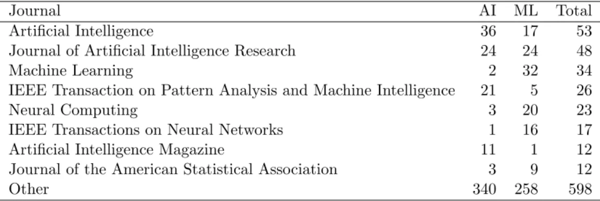
In this section, we provide a prototype analysis with thespapackage to illustrate the key func-tionality of this package on the Cora text data set (McCallum, Nigam, Rennie, and Seymore 2000). For these data, the observations are n= 827 text documents published predominantly in engineering, computer science and statistics journals. The attributes were generated elec-tronically on the web and then processed with in-house scripts. TheX information is 827×9 orthogonal matrix where Xik =I{paper iis in journal k}, for k= 1,· · ·,9 corresponding to the 8 journals listed in Table 1 plus a category for all other journals. The G information is a weighted graph represented by a co-citation network between the text documents. Specifi-cally, the adjacency matrix is constructed withAij =PI{iand j cite the same document}. The response is the binary indication that the specific document is classified to be about
Journal AI ML Total
Artificial Intelligence 36 17 53
Journal of Artificial Intelligence Research 24 24 48
Machine Learning 2 32 34
IEEE Transaction on Pattern Analysis and Machine Intelligence 21 5 26
Neural Computing 3 20 23
IEEE Transactions on Neural Networks 1 16 17
Artificial Intelligence Magazine 11 1 12
Journal of the American Statistical Association 3 9 12
Other 340 258 598
Table 1: Journal frequencies for the classes under consideration in the Cora text data.
machine learning (ML) or artificial intelligence (AI). The data are available as part of thespa
package.
To begin analysis, we provide the necessary preprocessing:
R> data("coraAI") R> y <- coraAI$class R> x <- coraAI$journals R> g <- coraAI$cite
R> keep <- which(as.vector(apply(g, 1, sum) > 1)) R> setdiff(1:length(y), keep) [1] 12 19 48 49 50 52 68 90 103 129 151 174 178 193 212 255 259 284 [19] 293 296 297 325 327 362 370 458 459 461 465 490 497 507 546 567 577 593 [37] 606 612 691 720 724 725 726 733 734 742 805 819 R> y <- y[keep] R> x <- x[keep,] R> g <- g[keep, keep] R> set.seed(100) R> n <- dim(x)[1] R> Ns <- as.vector(apply(x, 2, sum))
R> Ls <- sapply(1:length(Ns), function(i) sample(which(x[,i] == 1), R+ ceiling(0.035 * Ns[i])))
R> L <- NULL
R> for(i in 1:length(Ns)) L <- c(L, Ls[[i]]) R> U <- setdiff(1:n, L)
R> ord <- c(L, U) R> m <- length(L) R> y1 <- y
R> y1[U] <- NA
Observations 12, 19, · · ·, 819 were removed since they were isolated vertices. A stratified sample is used to insure that every journal is represented in labeled and unlabeled partitions.
Thespais used to fit an estimate on the observed graph directly without the journal indication matrix (i.e., ˆY = ˆf(G)):
R> A1 <- as.matrix(g)
R> gc <- spa(y1, graph = A1, control = spa.control(dissimilar = FALSE)) R> gc
Call:
spa(y1, graph = A1, control = spa.control(dissimilar = FALSE)) Sequential Predictions Algorithm (SPA) with training= 4 %
Type= soft Parameter= 1.968709 GCV type: approximate transductive Fit Measures:
RMSE= 2.439 tGCV= 8.646 tDF= 5.623 Transductive Parameters:
Regions: 0 Regularization: Inf Unlabeled Data Measures:
Training: 0.105 <=1 (Labeled/Supervised ~1) Unlabeled: 0.965 <=1 (No Supervised Equivalent)
The output provides several descriptive aspects of the model fit. First notice that, the fit used 4% of the data as labeled during training. The fit measures provide standard fit description with root mean squared error, parameter estimation type (refer to Section4) and transductive degrees of freedom. The transductive parameters were set to default, which means that the entire unlabeled data set was fit as one unit and no regularization was employed (i.e., FTF as a special case of SPA was employed). The unlabeled data measures provide a rough assessment of the potential usefulness of unlabeled data during training. The dissimilar flag must be
FALSE for thespa.control to indicate that the co-citation network is a similarity matrix. The natural concern is in the performance of the SPA onU (unlabeled set). To check perfor-mance onU, we calculate the misclassification error rate:
R> tab <- table(fitted(gc)[U] > 0.5, y[U]) R> 1 - sum(diag(tab)) / sum(tab)
[1] 0.4647355
The unlabeled error for this fit is extremely poor. An error this large typically indicates that the procedure is not using the unlabeled data appropriately during training. To investigate this, we provide a useful diagnostic by considering the AU L partition of A. This partition provides the common links between labeled-unlabeled data, and if an unlabeled observation
has no such links (i.e., AU Li ×1L = 0) then the observation cannot be utilized directly for
training. To assess the problematic unlabeled observations simply execute:
R> sum(apply(A1[U, L], 1, sum) == 0) / (n - m) * 100 [1] 39.92443
This tells us that nearly 40% of the cases have no direct associations with YL, which signifi-cantly deteriorates performance.
Next, we incorporate transductive prediction to account for unlabeled response estimates used in training by penalizing observations farther away from labeled cases. The idea is to sort the AU L×1L information and break the data into regions enumerated from highest (most associated) to lowest (least associated). In other words, the vectorAU L×1L provides a sorting method that groups objects to be classified at subsequent rounds similar to the shortest path used in the lattice example in Section2. The observations are then sequentially estimated, where at each round new unlabeled node estimates are treated as true values (refer to Section4.3for the general SPA or Section2for a simple example). To perform transductive prediction with thespa package use theupdate generic with the datargument:1
R> pred <- update(gc, ynew = y1, gnew = A1, dat = list(k = length(U),
+ l = Inf))
R> tab <- table(pred[U] > 0.5, y[U]) R> 1 - sum(diag(tab)) / sum(tab) [1] 0.2884131
The performance improves significantly. To update thespa object so that it corresponds to the above output execute:
R> gc <- update(gc, ynew = y1, gnew = A1,
+ dat = list(k = length(U), l = Inf), trans.update = TRUE) R> gc
Sequential Predictions Algorithm (SPA) with training= 4 % Transductive Parameters:
Regions: 794 Regularization: Inf Unlabeled Data Measures:
Training: 0.105 <=1 (Labeled/Supervised ~1) Unlabeled: 0.965 <=1 (No Supervised Equivalent)
1
The FTF algorithm is the special case of SPA where all observations are in one group and there is no regularization, that isdat = list(k = 0, l = Inf)produces the FTF output.
We see that, the transductive parameters are updated with the new fit. The training unlabeled measure of 0.105 does not change when using transductive prediction.
Next, we investigate the estimate ˆY =Xβˆ+ ˆf(G) where X is the journal indication matrix andG is the co-citation network. To execute this withspa:
R> gjc <- spa(y1, x, g, control = spa.control(diss = FALSE)) R> gjc
Sequential Predictions Algorithm (SPA) with training= 4 % Coefficients: other artificial_intelligence 0.369607329 0.049032222 machine_learning neural_computing 0.959096925 0.979303548 ieee_trans_Nnet ieee_tpami 0.947685447 0.012443001 j_artificial_intelligence_research ai_magazine 0.006865285 0.009279124 JASA 0.976590026 Transductive Parameters:
Regions: 0 Regularization: Inf
R> tab <- table((fitted(gjc) > 0.5)[U], y[U]) R> 1 - sum(diag(tab)) / sum(tab)
[1] 0.395466
The coefficient estimate is provided in the output and can be extracted using thecoefgeneric. The output also shows that the estimate suffers from the same performance problems with respect to the unlabeled data as the previous fit. As before, this problem can be fixed by using transductive prediction:
R> gjc1 <- update(gjc, ynew = y1, xnew = x, gnew = A1,
+ dat = list(k = length(U), l = Inf), trans.update = TRUE) R> gjc1
Sequential Predictions Algorithm (SPA) with training= 4 %
Type= soft Parameter= 1.968709 GCV type: approximate transductive Coefficients:
0.46182225 0.34495785 machine_learning neural_computing 0.86100990 0.91947929 ieee_trans_Nnet ieee_tpami 0.85709753 0.20706484 j_artificial_intelligence_research ai_magazine -0.05256496 0.11758127 JASA 0.62853374 Transductive Parameters:
Regions: 794 Regularization: Inf
R> tab <- table((fitted(gjc1) > 0.5)[U], y[U]) R> 1 - sum(diag(tab)) / sum(tab)
[1] 0.197733
As we can see the performance of the approach improved significantly after we updated the model to include transductive prediction. The strong performance on the unlabeled data suggests that using both the X information and G information contributed to predicting the class label of a document. In addition, a coefficient vector is obtained that may provide interpretable value for assessing a specific journal’s contribution to this classification problem.
4. Methodology
In Section3, we provided an analysis illustrating several features utilized by the spapackage. The output offers utilities useful for assessing and improving the fit, including transductive generalized cross validation and degrees of freedoms, influence of observations in U on ˆYL, an unlabeled contributionP
iI{AU Li×1L= 0}and a transductive prediction algorithm for
processing data. Next we present the details of the algorithmic fitting methodology, which will also provide some justification for these measures of fit.
The proposed approach essentially extends the concept of a linear smoother into the semi-supervised setting using the fitting the fits algorithm (the sequential predictions algorithm is a generalization for which the package is named and presented in Section4.3) (Culp and Michailidis 2008b). It is also quite similar to self-training approaches that use the expectation-maximization (EM) algorithm (Chapelle et al. 2006; Culp and Michailidis 2008b). The first step is to initialize the unlabeled vector ˆYU(0) =~0. Then the FTF iteratively fits:
ˆ YL(k+1) ˆ YU(k+1) ! = SLL SLU SU L SU U YL ˆ YU(k) ! , (1)
whereS is a linear smoother for response ˆY and is independent of k. Notice that the labeled response estimate is reset toYL before fitting, which intuitively allows the procedure to train with the observed response (known response) and use the previous estimated response fit
where the responses are unobserved (unknown). The algorithm is repeatedly executed until global convergence defined byk YˆU(k+1)−YU(k) k< with >0. The vector ˆY = [ ˆYL>,YˆU>]> denotes the convergent solution to (1). To establish global convergence, notice that at step k
we have that ˆY(k) =Pk−1
`=0SU U` SU LYL+SU Uk Yˆ
(0)
U and therefore the geometric matrix series is guaranteed to converge whenever ρ(SU U) <1 where ρ is the spectral radius. The closed form convergent solution can be obtained as the limit on the geometric matrix series: ˆYL=
SLLYL+SLUYˆU and ˆYU = (I−SU U)−1SU LYL.
Thespa package primarily fits stochastic based smoothers including kernel smoothers, graph smoothers and a semi-parametric extension involving kernel smoothing. However, before we study kernel smoothers in the semi-supervised setting, we first look at linear regression to gain important insight into the procedure, since several key aspects of the spa package are motivated from linear regression. Upon presenting FTF with linear regression (Section4.1), we then focus on kernel smoothing and graph smoothing (Section 4.2), the full sequential predictions algorithm (Section4.3), and semi-parametric smoothing (Section4.4) in the semi-supervised setting.
4.1. Example: Fitting the fits with linear regression
Next we study linear regression in the semi-supervised setting to provide insight and motivate key results, including transductive degrees of freedom and transductive generalized cross-validation. To implement semi-supervised linear regression, one must apply the hat matrix
H =X(X>X)X>= XL(X>X)−1XL> XL(X>X)−1XU> XU(X>X)−1XL> XU(X>X)−1XU> = HLL HLU HU L HU U
as the smoother in (1). Note the supervised hat matrix is HeLL =XL(XL>XL)−1XL>.
Semi-Supervised linear regression with FTF is quite simple to fit inR, using the.GlobalEnvnested insapplycommand: R> set.seed(100) R> x <- matrix(rnorm(40), 20) R> z <- cbind(x, 1) R> y <- z %*% rnorm(3) + rnorm(20, , 0.5) R> H <- z %*% solve(t(z) %*% z, t(z)) R> L <- 1:5 R> U <- 6:20 R> yh <- c(y[L], rep(0, 15)) R> ftfls <- function(i) { + .GlobalEnv$yh[L] <- y[L] + .GlobalEnv$yh <- H %*% .GlobalEnv$yh + } R> ftfres <- sapply(1:200, ftfls) [1] -1.8053630 -0.7672166 ... -0.9983772
Upon convergence an estimate for the response is obtained in closed form with ˆYU = (I −
The natural question to ask is, “What are the properties of the convergent solution for lin-ear regression with FTF?” The answer is clarified by comparing our result to the ordinary supervised least squares solution:
R> dat <- data.frame(y = y, x)
R> supls <- predict(lm(y ~ ., data = dat, subset = L), newdata = dat) R> apply((ftfres - supls)^2, 2, sum)[c(1:2, 199:200)]
[1] 2.831134e+01 1.668253e+01 ... 8.545281e-15 7.265162e-15
By iteration 200 the difference between the two is negligible and therefore we see that semi-supervised linear regression using FTF reduces to the semi-supervised least squares solution. This equivalency is proven for the generalized linear model in Culp and Michailidis (2008b). A similar result can be shown when treating the semi-supervised linear regression problem as a missing data problem (Little and Rubin 2002, p. 29)
The equivalency between semi-supervised linear regression using FTF and supervised ordinary least squares results in two new expression for the hat matrix. The equivalent hat matrices are given by:
e
HLL = XL(XL>XL)−1XL> (supervised) (2) = HLL+HLU(I−HU U)−1HU L(transductive) (3) = HLL+HeU L> HU L (approximate transductive) (4)
where HeU L = XU(XL>XL)−1XL> (supervised unlabeled estimate). Upon convergence each
formulation has the same error and the same trace. The degrees of freedom of the residuals of the semi-supervised estimator are defined as
df =|L| −tr(HLL+HLU(I −HU U)−1HU L) =|L| −p
since this form yields the smoother for the labeled estimator resulting from FTF, i.e., ˆYL=
HLL+HLU(I−HU U)−1HU L
YL.
This equivalency between these projection matrices is useful in computing the generalized cross-validation (GCV) error rate of a smoother, i.e., the GCV for smootherS is defined as:
GCV(S) = kYL−SYLk22
(1−tr(S)/|L|)2.
To do this, we define GCV with reference to (2) as labeled GCV ("lGCV"), GCV with refer-ence to (3) as transductive GCV ("tGCV"), and GCV with reference to (4) as approximate transductive GCV ("aGCV"). All of these measures provide an identical value in linear regres-sion but will differ in kernel smoothing (refer to Section 4.2). The "tGCV" criterion would be the best choice but is computationally demanding due to the need for (I−HU U)−1. We recommend using the approximate transductive GCV criterion since it is less demanding computationally and is still influenced by observations in U. The choice of GCV is set by
spa.control with"aGCV" as the default.
Remark: Linear regression is not implemented in the spa package since the lm command computes it equivalently.
4.2. Semi-supervised stochastic kernel smoothing
Next we study kernel smoothers, where a kernel function is applied directly to distances in
X withWij =Kλ(xi, xj) whereKλ(xi, xj) = exp(−dij/λ) is default. In generalλis a tuning parameter whereλ≈0 tends to yield solutions with low bias and high variance while λ→ ∞
tends to yield solutions with high bias and low variance. The matrixW emits the partition fori, j∈L∪U: W = WLL WLU WU L WU U .
The FTF algorithm allows for the observations inWU U,WU L, andWU L> to influence training of the procedure, by iteratively fitting (i) ˆYL(k−1)=YL and (ii) ˆY(k) =SYˆ(k−1) withS =D−1W whereDis the diagonal row sum matrix ofW (denoted asD= diag(W1)) and initialization
ˆ
YU(0). Tracing the iteration, we get that the unlabeled estimator is ˆYUk =Pk−1
`=0 SU U` SU LYL+
SkU UYˆU(0) and take the limit ask→ ∞to get the closed form solution, ˆY = ˆY(∞):
ˆ YL ˆ YU = SLL+SLU(I−SU U)−1SU L (I −SU U)−1SU L YL. (5)
The condition for producing a stable estimator is discussed in Section4.3.
Unlike in linear regression, ˆYL is not equivalent to the supervised estimator. However, the supervised estimator is influential on the result as we show next. First for kernel regression we have that S = D−1W. Define DL, DU as the respective labeled/unlabeled diagonal submatrices of the diagonal row-sum matrix D. In addition, denote DLL = diag(WLL1L), that is the row sum matrix of WLL, and similarly denote DLU = diag(WLU1U), DLU = diag(WLU1U), and DU U = diag(WU U1U). From this, DL =DLL+DLU and DU =DU U +
DU L. Next, we denote the supervised kernel smoother asTLL=DLL−1WLL and the supervised prediction smother asTU L =D−U L1WU L. The supervised estimator is denote byYe. To connect
supervised estimation to ˆYL we have that: ˆ YL = D−L1DLL TLLYL+ I−DL−1DLL SLU LYL ≡ QYeL+ (I−Q) ˘YL, (6)
whereQ =DL−1DLL ≤I and SLU L = DLU−1WLU(I −SU U)−1SU L. From this decomposition, we notice that if Q≈I then the supervised labeled estimate is close to the semi-supervised labeled estimate. On the other hand, shrinking this matrix provides more influence with
SLU L. It is easy to show that SLU L is right stochastic and therefore (6) is an average of two right stochastic matrices which is also right stochastic. The value ¯Q≡ tr(|LQ|) provides a quick determination of the effect of the unlabeled data on the labeled estimate in training and is provided in the output of thespa object (0.105 for the Cora data). Values near one indicated that (6) is close to YeL =TLLYL (supervised) while smaller values indicate that the estimate
of ˆYLis influenced by ˘YL.
For the kernel smoothing problem, we are also interested in approximating the matrixSLU L without requiring the computation of the inverse (for λ estimation). Using the linear re-gression result, we employ SLU L ≈ V−1TU L> SU L = V−1TU L> (I −D−U1DU U)TU L, where V is the appropriate matrix to make the approximation right stochastic. This adjustment is ex-tremely useful for fitting GCV as it is used bytype = "aGCV"and is default forspa.control.
This result in the case of kernel regression is not equivalent to GCV using the transductive smoother or GCV using the labeled smoother (refer to Section4.1).
Graph-based smoothing is a natural generalization of kernel smoothing. The adjacency matrix of the graph is given by A and the smoother is obtained as S = D−1A. The FTF is then applicable in the same manner as with the kernel smoothing approach discussed previously (i.e., A and W are quite similar). One key difference between graph-based smoothing and kernel smoothing is that the graph problem is inherently semi-supervised (often referred to as transductive in this special case), and therefore a supervised alternative does not exists. Care is taken with the design of thespa to allow for transducitve prediction when necessary.
4.3. The sequential predictions algorithm
The FTF algorithm was previously employed with smoothers. The full sequential predictions algorithm is an extension of FTF to perform transductive prediction with the intent of im-proving performance (refer to Cora example). Transductive prediction addresses the issue of updating a classification or regression technique to incorporate either new observations (labeled or unlabeled) unavailable originally during training, reassess the current unlabeled observations used previously during training, or both.
To motivate the need for the SPA algorithm, we first consider the circumstances for when (I−SU U)−1is expected to be unstable. To provide insight recall that the smootherS =D−1W
is right stochastic, i.e.,
SLL SLU SU L SU U 1L 1U = 1L 1U and Sij ≥0.
In such a circumstance, a stable estimator is achieved wheneverSU U1U <1U (i.e., the sum of each row inSU U is less than one). From the above equation we observe that the requirement is satisfied whenever SU L1L >0L (i.e., every row in SU L sums to a positive number). The instability occurs wheneverSU L1L≈0L or sufficientlyWU L×1L≈0L. This condition can easily be violated in practice. For example, a compact kernel could force weak connections between labeled and unlabeled data to vanish. It is also common to employ a non-compact kernel and then ak-nn function to that kernel (known as ak-nn graph), which results in the analogous effect. In the case of an observed graph, it is not difficult to obtain a vertex that is only connected to other unlabeled vertices (refer to the Cora text data). This problem becomes worse as|L|decreases for each of these examples, since there are less labeled cases to connect with the unlabeled cases.
To correct for this we extend the FTF algorithm into the sequential predictions algorithm (Culp and Michailidis 2008a). The main idea is to sortWU L×1Land partition the unlabeled dataU ={U(`)}k
`=1 intokdisjoint sets such that the set with the most labeled connectivity is employed first with FTF. In other words, apply FTF with labeled casesL(0)=Land unlabeled cases inU(1). Then treat the unlabeled estimates as true and at iteration ` train FTF with labeled cases L(`) = L(`−1) ∪U(`) and unlabeled set U(`+1). This process repeats with a total ofkcalls to FTF. InCulp and Michailidis (2008a), we provide a penalty function based on constrained regularization to correct for the use of unlabeled predictions at subsequent rounds. The main idea is to increasingly push the estimates towards a global point estimates (mean ofYL) as the algorithm progresses. This entire approach is implemented in the update generic, requiring parameterdat = list(k = 0, l = Inf)by default with subparametersk
(number of regions) andl(inverse regularization penalty, i.e.,l = 0is infinite regularization while l = Infis no regularization). The approach is shown to work quite well for the Cora text data and was also shown to be competitive to several state-of-the-art graph-based semi-supervised approaches. An extension to hard labels based on exponential loss is also discussed inCulp and Michailidis(2008a) and is implemented in spa (use type = "hard" forspacall andreg = "hlasso" forupdate).
4.4. An optimization framework for the semi-parametric model
The fitting the fits algorithm provides a simple and effective way to fit data with an unlabeled partition and or graph based terms. The connection to optimization is now established for fitting semi-parametric models. In order to do this, we first establish the link between the FTF algorithm and optimization. Then we generalize this approach to the more general semi-parametric problem.
For this, denoteφ(y, f) = (y−f)2as the squared error loss function, and consider the following optimization problem: min f X i∈L φ(yi, fi) +λf>P f,
whereP is a positive semi-definite penalty matrix. In this construct the loss is incurred from the labeled estimator fL to the observed response YL, while the full function is accounted for with the penalty term. The penalty matrix P is taken as the combinatorial Laplacian
P = ∆≡D−W for observed graph and constructed graph terms.
Next we demonstrate that the FTF algorithm with kernel regression does indeed solve the following optimization problem:
min
f (YL−fL)
>
WLL(YL−fL) +f>∆f.
Define, Y(YU) = [YL, YU] with YU an arbitrary unlabeled response. Then we have that (YL−fL)>WLL(YL−fL) = (Y(fU)−f)>W(Y(fU)−f) for allf and is independent of fU. From this, the derivative solves−W(Y( ˆfU)−fˆ) + ∆ ˆf =~0. Rearranging we get that:
ˆ fL ˆ fU = SLL SLU SU L SU U YL ˆ fU ,
where S = (W + ∆)−1W = D−1W. Solving the fixed point ˆfU = SU UfˆU +SU LYL and plugging the solution back in yields the identical solution to (5) for kernel regression.
Using this approach, we then motivate the semi-parametric model η = Xβ +f(G) as the solution to: min f,β X i∈L (YL−fL−XLβ)>WLL(YL−fL−XLβ) +f>∆f.
As we proceeded in kernel regression, we have that (Y(ηU)−η)>W(Y(ηU)−η) = (YL−
ηL)WLL(YL−ηL) and is independent of ηU. Taking the gradient with respect to f we get that
Taking the gradient with respect toβ and substituting for f we get that:
−X>W(Y(ηU)−η) =~0 =⇒ X>W(I−S)Xβ=X>W(I−S)Y(ηU).
From this, we get that ˆη=Xβˆ+ ˆf =Xβˆ+S(Y(ˆηU)−Xβˆ) =H(S)Y(ˆηU) for some smoother
H(S). From this, the FTF for the semi-parametric estimator reduces to: initialize ˆηU(0)
and repeat, (i) ˆηL(k) = YL and (ii) ˆη(k+1) = H(S)ˆη(k). Convergence is guaranteed when-ever ρ(H(S)U U) < 1. The SPA algorithm naturally applies to the semi-parametric model where the estimates forβ are built up over the kcalls based on the order ofWU L×1L.
5. The
spa
package
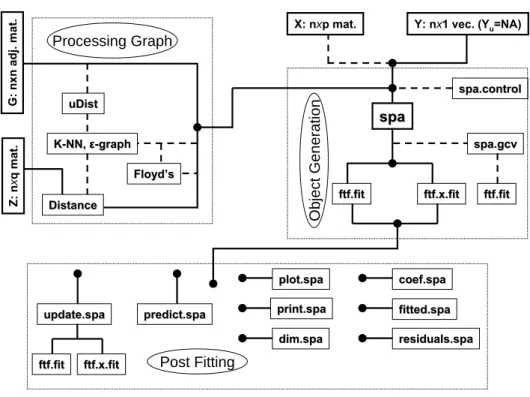
The spa package provides semi-supervised functions in R to fit and evaluate an estimate of the form ˆY = ˆf(G) or ˆY =Xβˆ+ ˆf(G), where ˆβ is the coefficient vector, ˆY is the estimated response, and ˆf is a function defined over the vertices ofG. The process is broken into three key phases: (i) processing the graph, (ii) object generation and (iii) post fitting (refer to Figure 2). The first phase provides a series of functions for processing an observed graph (refer to the Cora example above) or a graph constructed from the Z data. The second phase is generating thespa object with the tuning parameter estimation functionality. The third phase provides post fitting functions featuring transductive prediction with theupdate
generic, inductive prediction with thepredictgeneric, and a series of other standard generic functions. spa spa ftf.fit ftf.fit Distance Distance Floyd’s Floyd’s K K--NN, NN, εε--graphgraph uDist uDist Processing Graph
X: nxp mat. Y: nx1 vec. (Yu=NA)
Z: n x qm at . G: n xn adj. mat. Object Generation ftf.x.fit ftf.x.fit spa.gcv spa.gcv ftf.fit ftf.fit update.spa
update.spa predict.spapredict.spa
ftf.fit
ftf.fit ftf.x.fitftf.x.fit
spa.control spa.control plot.spa plot.spa print.spa print.spa dim.spa dim.spa coef.spa coef.spa fitted.spa fitted.spa residuals.spa residuals.spa Post Fitting
Figure 2: Sequence diagram for describing the relationship between the functions in the spa
0 1 2 3 4 5 6 −6 −4 −2 0 2 x1 x2 ● ● ● ● ● ● ● ● ● ● ● ● ● ● ● ● ● ●● ● ● ● ● ● ● ● ● ● ● ● ● ● ● ● ● ● ● ● ● ● ● ● ● ● ● ● ● ● ● ●● ● ● ● ● ● ● ● ● ● ● ● ● ● ● ● ● ● ● ● ● ● ● ● ● ● ● ● ● ● ● ● ● ● ● ● ● ● ● ● ● ● ● ● ● ● ● ● ● ● ● ● ● ● ● ● ● ● ● ● ● ● ● ● ● ● ● ● ● ● ● ● ● ● ● ● ● ● ● ● ● ● ● ● ● ● ● ● ● ● ● ● ● ● ●● ● ● ● ● ● ● ● ● ● ● ● ● ● ● ● ● ● ● ● ● ● ● ● ● ● ● ● ● ● ● ● ● ● ● ● ● ● ● ● ● ● ● ● ● ● ● ● ● ● ● ● ● ● ● ● ● ● ● ● ● ● ● ● ● ● ● ● ● ● ● ● ● Y^= f^((GX)) YL=f((XL))++ εε Y^= f^((GX)) YL=f((XL))++ εε
Two Moon Simulated Data
Inductive Prediction with a Transductive Model
0 1 2 3 4 5 6 −6 −4 −2 0 2 x1 x2 ● ● ● ● ● ● ● ● ● ● ● ● ● ● ● ● ● ●● ● ● ● ● ● ● ● ● ● ● ● ● ● ● ● ● ● ● ● ● ● ● ● ● ● ● ● ● ● ● ●● ● ● ● ● ● ● ● ● ● ● ● ● ● ● ● ● ● ● ● ● ● ● ● ● ● ● ● ● ● ● ● ● ● ● ● ● ● ● ● ● ● ● ● ● ● ● ● ● ● ● ● ● ● ● ● ● ● ● ● ● ● ● ● ● ● ● ● ● ● ● ● ● ● ● ● ● ● ● ● ● ● ● ● ● ● ● ● ● ● ● ● ● ● ●● ● ● ● ● ● ● ● ● ● ● ● ● ● ● ● ● ● ● ● ● ● ● ● ● ● ● ● ● ● ● ● ● ● ● ● ● ● ● ● ● ● ● ● ● ● ● ● ● ● ● ● ● ● ● ● ● ● ● ● ● ● ● ● ● ● ● ● ● ● ● ● ● ● ● ● ● ● ● ● ● ● ● ● ● ● ● ● ● ● ● ● ● ● ● ● ● ● ● ● ● ● ● ● ● ● ● ● ● ● ● ● ● ● ● ● ● ● ● ● ● ● ● ● ● ● ● ● ● ● ● ● ● ● ● ● ● ● ● ● ● ● ● ● ● ● ● ● ● ● ● ● ● ● ● ● ● ● ● ● ● ● ● ● ● ● ● ● ● ● ● ● ● Original Updated Original Updated
Figure 3: Scatterplot for two variables X1 and X2 with the class label as light gray, dark gray, or missing (small gray circle). (left) A supervised kernel smoother is gray, and the SPA fit is black. (right) Transductive prediction with the spa, the original fit for the two moon data set is provided as black, while the retrained spawas gray and dashed.
To illustrate the key functions necessary for fitting a model with thespa package we consider a synthetic two moon data set (refer to Figure 3). The unlabeled data are generated based on the intuitive cluster assumption: If the classes are linearly separable then observations on similar clusters should share the same label. In this example, the SPA breaks the unlabeled data into two moon-like clusters, a separation that cannot be found by the supervised kernel smoother.
To load the data inRexecute:
R> library("spa") R> set.seed(100)
R> dat <- spa.sim(type = "moon")
The three phases for spa presented in Figure 2are each discussed in detail for these data.
5.1. Processing graph
The graph processing stage highlighted in Figure2provides the means necessary for preparing the Z information or an observed graph for processing with thespa function. The functions for manipulating these data consist of uDist,knnGraph,epsGraph, and floyd.
In the case of an observed graph, this step accounts for several diverse types of similarity graphs. For example, if the graph were sparse (e.g., a planar graph) then one may wish to employ the shortest path distance metric on the graph using the uDist function. The purpose of performing this manipulation with a sparse graph is to relate distant nodes with a distance proximity measure through neighboring links. As a consequence the unlabeled observations that were not originally directly linked to labeled cases may now have associations
through neighboring unlabeled observations that were connected with labeled cases. On the other hand, when the graph is dense, like with the Cora example, this type of manipulation is not necessary and in our experience can hinder performance. If the uDist function is employed with an observed graph, then the dissimilar flag in thespa.control must remain
TRUEotherwise it must be set to FALSE.
In the case of convertingZ information to a graph, the first step is to specify an appropriate distance metric onZ. For the simulated data, we would employ Euclidean distance:
R> Dij <- as.matrix(daisy(dat1[, -1]))
For Z matrices with large q, restricting to local connectivity with a k-nn or graph can significantly improve performance of this technique (Tenenbaum, Silva, and Langford 2000). However, thek-nn object is not a proper distance metric, and we often wish to convert into a proper metric with Floyd’s algorithm (the triangle inequality does not hold for ak-nn graph). To do this withspa execute:
R> DNN <- knnGraph(Dij, dist = TRUE, k = 5) R> DFL <- floyd(DNN)
The flagdist = TRUE indicates that the object is distance weighted.
Upon obtaining the appropriate graph representation for the spafunction, we focus next on generating a spa object. Notice the other spa input parameters, Y and X, require minor processing. ForY, set YU =N Aand make sureX is either adata.frameormatrix.
5.2. Generating a spa object
The spaobject encapsulates the model fit by the procedure. This step accounts for param-eter estimation, problematic unlabeled data, and object generation. The paramparam-eter estima-tion procedure is designed to estimate parameters efficiently using one of four generalized cross-validation measures with either a bisection algorithm or grid search. The problematic unlabeled data cases (WU Li×1L = 0) are carefully identified and handled with the global
argument. The final object is then generated, reporting several useful measures that de-scribe the current fit. The functions employed here include spa.control, spa and internal GCV/fitting functions.
For parameter estimation, one must first consider the spa.control function. For this, the specified GCV is optimized over a set of potentialλcandidates, or a value is provided using the ltval option. To determine the set of potential candidates we provide a fast bisection algorithm and a slow, more thorough, grid search. For the bisection algorithm the key pa-rameters are lqmax = 0.2, lqmin = 0.05, ldepth = 10, and ltmin = 0.05. The lqmax
and lqmin set a range to search based on the [lqmin, lqmax] ·100 quantile of the density taken on finite distances. In our experience, this provides a fairly good spread of potentialλ
candidates. In some cases, the quantile determined bylqminis negative due to a large density at zero, and one can set the parameter ltmin to correct for this. The bisection algorithm recursively divides the interval in half and finds the subinterval that contains the minimum GCV. This process is repeated ldepth times. The approach is fast and usually works well. However the algorithm can get stuck and arrive at aλestimate that is unsuitable. To correct for this, a uniform search over a grid of sizelgridbetween thelqmintolqmaxquantiles can be performed to estimateλ.
The object generation required specification of the unlabeled data. This can be done in two ways. First a labeled set of indices can be provided using the L argument, and the second approach is to set YU = N A. The algorithm processes a supervised kernel smoother if no unlabeled data are specified. To generate thespaobject with the simulated moon example, we execute the following command inR:
R> L <- which(!is.na(dat$y)) R> U <- which(is.na(dat$y))
R> gsup <- spa(dat$y[L], graph = Dij[L, L]) R> gsemi <- spa(dat$y, graph = Dij)
First we consider the supervised kernel smoother fit on only the labeled data:
R> gsup
Sequential Predictions Algorithm (SPA) with training= 100 % Type= soft Parameter= 0.04219128 GCV type: labeled
....
Unlabeled Data Measures:
Training: 1 <=1 (Labeled/Supervised ~1) Unlabeled: NaN <=1 (No Supervised Equivalent)
For the supervised kernel smoother, the parameterλwas estimated as 0.04. Notice also that if no unlabeled data are specified then the parameter estimation defaults to using labeled GCV. In addition, the unlabeled data measures have no meaning here. The supervised kernel smoother result is shown as the gray curve in both panels of Figure 3. Notice that this estimate completely misses the moon like structure in the left figure.
Next, we consider the semi-supervisedspa fit on the moon data:
R> gsemi
Sequential Predictions Algorithm (SPA) with training= 3 %
Type= soft Parameter= 0.05 GCV type: approximate transductive ...
Unlabeled Data Measures:
Training: 0.848 <=1 (Labeled/Supervised ~1) Unlabeled: 0.995 <=1 (No Supervised Equivalent)
The approximate GCV is used to estimate λ as 0.05. The first unlabeled data measure is 1
|L|tr(D −1
panel of Figure 2. Here the use of the unlabeled data produces a classification border that separates the moon-like data clusters.
To view the GCV path for parameter estimation consider theparm.eststructure:
R> gsemi$model$parm.est
$cvlam [1] 0.05 $gcv
[1] 3.414852e-29 2.327041e-01 2.396981e-02 4.819773e-04 5.030481e-07 [6] 2.823065e-11 3.441998e-16 9.467595e-21 1.006386e-20 6.494275e-20 $lambda
[1] 0.05000000 1.27511510 0.66255755 0.35627877 0.20313939 0.12656969 [7] 0.08828485 0.06914242 0.05957121 0.05478561
We see that the approach considered several values ofλbefore settling onλ= 0.05.
5.3. Post fitting
The spa package provides several enhancements for processing a spa object post fitting. Most are standard generic methods associated with models in general. The main focus is on transductive and inductive prediction. The generics available at this stage are: update,
predict,plot,print,dim,coef,fitted, and residuals.
For inductive prediction, thepredict generic is designed to process a new vertex, where the edges for this observation with respect to the original labeled and unlabeled observations are assumed to be available. That is, let w·j be the edge network for predicting vertex ·, and form the prediction as ˆY·=
P j∈L∪Uw·jYˆj P j∈L∪Uw·j with ˆY = [Y > L ,Yˆ > U ]
>. Next we illustrate inductive
prediction for observation x= (0 0) withspa.predict:
R> newobs <- c(0, 0)
R> newnode <- as.matrix(sqrt(apply(cbind(dat$x1 - newobs[1], + dat$x2 - newobs[2])^2, 1, sum)))
R> round(predict(gsemi, gnew = newnode), 3)
[1] 0
One could also process a sequence of new data points at once, e.g., to predict (4,−4), . . . ,
(4,4),(4,5) execute:
R> newnodes <- sqrt(t(sapply(1:10 - 5,
+ function(j) (dat$x1 - 4)^2 + (dat$x2 - j)^2))) R> round(predict(gsemi, gnew = newnodes), 3)
Figure 4: A synthetic Swiss Roll classification set. The true classes are provided on the left, and thek= 6 nearest neighbor graph is given on the right.
One could classify these observations according to the above probability class estimates. Transductive prediction (updating) is more complex. In this case the observations provide inherent meaning and the current classifier should be modified to incorporate them. The object is changed post fitting, and therefore this type of prediction is really an update. The purpose of this update could be to perform the general SPA on the observations used for training with different settings or to perform the general SPA with new observations (labeled or unlabeled). The key parameters other than the (y, x, G) data for retraining include dat
and trans.update. The dat parameter is a list with two components: k = 0 and l =Inf (default). The parameterk controls the number of regions to break U into, while l controls the regularization for penalizing estimates based on its regions (regions farther from the original L get higher regularization). To update with a new unlabeled data set generated from the same underlying data mechanism, execute:
R> dat <- rbind(dat, spa.sim(100, 0))
R> gsemi <- update(gsemi, ynew = dat$y, , as.matrix(daisy(dat[, -1])), + trans.update = TRUE)
TheRcontour plot for the new updated border is given in Figure3 (right).
6. Examples
6.1. Swiss roll data set
For the first example, we present a simulation where the variables in theXdata lie on a swiss roll manifold (refer to Figure 4, left). For the response, we first define a sequence of regions denoted by indexithen the classification rule is defined as the indicator that an observation is on an even region. Refer to Figure4(left) for the region breakdown. The technical details
for the example are as follows: let z1 ∼ U[0,5∗π] and z2 ∼U[6,10] then we have that the manifold is generated withx1 =z1sin(z1),x2 =z1cos(z1), andx3 =z2−8. For classification, setx2 =P3
i=1x2i and then generate the response with:
y[(x2<15(i+ 1) & x2 ≥15i)] = (imod 2) (7) wherei= 0 to dmaxix2i
15 e.
TheRcode necessary to generate the example is given below:
R> library("scatterplot3d") R> n <- 1000 R> set.seed(100) R> z1 <- runif(n, 0, 5 * pi) R> z2 <- runif(n, 6, 10) R> x1 <- z1 * sin(z1) R> x2 <- z1 * cos(z1) R> x3 <- z2 - 8 R> x <- cbind(x1, x3, x2) R> xsq <- apply(x^2, 1, sum) R> y <- rep(100, n) R> inc <- 15 R> p1 <- ceiling(max(xsq)/inc)
R> for(i in 0:p1) y[xsq < inc * (i + 1) & xsq >= i * inc] = i %% 2 R> gr <- gray(c(0.3, 0.7))[y + 1]
R> scatterplot3d(x1, x3, x2, ylim = c(-8, 8), color = gr, pch = 16, + cex.symbols = 1, cex.axis = 1.2, angle = 30)
R> title("Simulated Swiss Roll", cex.main = 2) R> title("\n\nTrue Classes")
R> g1 <- knnGraph(x, k = 6, weighted = FALSE)
R> pl <- scatterplot3d(x1, x3, x2, ylim = c(-8, 8), color = gr, pch = 16, + cex.symbols = 1.2, type = "n", cex.axis = 1.2, angle = 45)
R> for(i in 1:n) {
+ ind <- which(g1[, i] > 0) + for(j in 1:length(ind)) {
+ pnts <- pl$xyz.convert(c(x[i, 1], x[ind[j], 1]), + c(x[i, 2], x[ind[j], 2]), c(x[i, 3], x[ind[j], 3])) + lines(pnts$x,pnts$y, col = 1, lwd = 1.5, lty = 1)
+ }
+ }
R> title("Simulated Swiss Roll", cex.main = 2) R> title("\n\nk=6 Nearest Neighbor Graph")
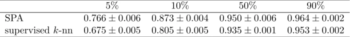
The preprocessing for this example included generating a k = 6 nearest neighbor graph using the Euclidean distance metric and applying Floyd’s algorithm to the graph (refer to the right panel of Figure 4 for the k-NN graph). These settings captured the manifold. For classification, we computed the true unlabeled classification accuracy averaged over 50 simulations. For this, the labeled size varied among 5%, 10%, 50%, and 90%. The results of the simulation are given in Table2.
5% 10% 50% 90% SPA 0.766±0.006 0.873±0.004 0.950±0.006 0.964±0.002 supervisedk-nn 0.675±0.005 0.805±0.005 0.935±0.001 0.953±0.002
Table 2: Accuracy rates for simulation.
The results for thek= 6 supervised nearest neighbors algorithm was also included for com-parison purposes. For these data, we see thatspa outperforms the supervisedk-nn especially when the|L|is small. A single run with 10% labeled is given below:
R> g6 <- knnGraph(x, k = 6) R> Dij <- floyd(g6) R> set.seed(100) R> L <- sample(1:n, ceiling(0.1 * n)) R> U <- setdiff(1:n, L) R> y1 <- y R> y1[U] <- NA
R> gself <- spa(y1, graph = Dij)
R> tab <- table(fitted(gself)[U] > 0.5, y[U] > 0.5) R> sum(diag(tab)) / sum(tab)
[1] 0.72
6.2. Protein interaction data set
For this next example, the observations consist of 1875 proteins from yeast organisms in the form of a graph. For this particular data 13 different systems are used to detect interactions between any two-proteins, e.g., a protein interaction could be detected by two-hybrid, im-munoprecipitation, affinity-purification, etc (Rueppet al.2004). The edges for this graph are defined by the count of interactions detected from different systems, i.e.,eij is given by:
eij =
X
s
1{systemsdetects interaction between proteini,j},
It is assumed that each system would detect an interaction between two identical proteins, i.e., eii = 13 for all i. The response for this data set is the classification of whether the protein is located on a nucleus of the cell. For these data, we do not have the response for 685 observations. The goal is to use the protein interaction network to classify the cell location for these observations. The followingRcode reads in the data:
R> data("protLoc") R> y <- protLoc$class R> gs <- protLoc$inter R> A <- gs[[1]] + gs[[2]] R> diag(A) <- 13 R> resp <- as.data.frame(sapply(1:nlevels(y), + function(i) as.numeric(y == levels(y)[i])))
R> names(resp) <- levels(y) R> y <- resp[, 20]
R> n <- length(y)
Next we fit the SPA to these data. To assess performance we generate a training set and a tuning set with 50% of the non-missing cases in both.
R> set.seed(100) R> L <- sample(which(!is.na(y)), 0.5 * n) R> tuneind <- setdiff(which(!is.na(y)), L) R> uind <- which(is.na(y)) R> U <- c(tuneind, uind) R> y1 <- rep(0, n) R> y1[L] <- y[L] R> y1[U] <- NA
R> g <- spa(y1, graph = A, control = spa.control(diss = FALSE)) R> tab <- table(y[L], fitted(g)[L] > 0.5)
R> a1 <- sum(diag(tab)) / sum(tab)
R> tab <- table(y[U], fitted(g)[U] > 0.5) R> a2 <- sum(diag(tab)) / sum(tab)
R> a3 <- sum(apply(A[U, L], 1, sum) == 0) / (length(U)) * 100
R> cat("Labeled Acc.=", round(a1,4), " \nUnlabeled Acc.", round(a2, 4), + " \n% zero A_ULx 1=", round(a3, 4), "\n")
Labeled Acc.= 0.9989 Unlabeled Acc.= 0.77 % zero A_ULx 1= 41.0448
From these results, we notice that the labeled accuracy is 0.999 and the unlabeled accuracy on the tuning set is 0.77. In addition, 41% of the unlabeled cases have no direct link to the labeled response. Updating using transductive prediction addresses this issue and can improve the fit. We use the tuning set to optimize the SPA regularization parameter settings for ` and k. In the case of ties, we choose the smallest k and largest ` to yield the least regularization.
R> levs <- c(0, 5, 10, 100, length(U)) R> lss <- c(seq(0, 100, length = 7), Inf)
R> tunes <- matrix(0, length(levs), length(lss)) R> t1 <- proc.time()
R> for(j in 1:length(levs)) { + for(i in 1:length(lss)) {
+ g1 <- update(g, ynew = y1, gnew = A, dat = list(k = j, l = lss[i])) + tab <- table(g1[U] > 0.5, y[U])
+ tunes[j, length(lss) - i + 1] <- sum(diag(tab)) / sum(tab) + cat("j=", j, " i=", i, "time=", (proc.time() - t1) / 60, "\n")
+ }
j= 1 i= 1 time= 0.01533333 0.003016667 0.01075 0 0 j= 1 i= 2 time= 0.0302 0.00535 0.02081667 0 0 ...
j= 7 i= 4 time= 0.6144167 0.1131833 0.4250333 0 0 R> tlev <- unique(apply(tunes, 1, which.max)) R> tls <- apply(tunes[,tlev], 2, which.max) R> i1 <- which.max(diag(tunes[tls, tlev])) R> olev <- tls[i1]
R> otls <- tlev[i1]
R> gprot <- update(g, ynew = y1, gnew = A, dat = list(k = olev, l = otls), + trans.update = TRUE)
R> tab <- table(y[L], fitted(gprot)[L] > 0.5) R> a1 <- sum(diag(tab)) / sum(tab)
R> tab <- table(y[U], fitted(gprot)[U] > 0.5) R> a2 <- sum(diag(tab)) / sum(tab)
R> cat("Labeled Acc.=", round(a1, 4),
+ " \nUnlabeled Acc.=", round(a2, 4), "\n") Labeled Acc.= 0.9989
Unlabeled Acc.= 0.78
From this result, we notice some improvement with the SPA over the FTF algorithm directly. Using this SPA fit we then get the following as the predictions for the unlabeled responses.
R> round(fitted(gprot)[uind],4) [1] 0.3725 0.4493 ... 0.6312 0.1688
7. Concluding remarks
In this paper, an R package spa that implements a semi-supervised framework for fitting parametric models was presented. Its key features are parameter estimation in semi-supervised learning, the distinction between transductive and inductive prediction, and a variety of functions for processing a graph.
References
Belkin M, Matveeva I, Niyogi P (2004). “Regularization and Semi-Supervised Learning on Large Graphs.” InCOLT, pp. 624–638.
Blum A, Chawla S (2001). “Learning from Labeled and Unlabeled Data Using Graph Min-cuts.” InInternational Conference on Machine Learning, pp. 19–26.
Blum A, Mitchell T (1998). “Combining Labeled and Unlabeled Data with Co-Training.” In
Computational Learning Theory, pp. 92–100.
Chapelle O, Sch¨olkopf B, Zien A (eds.) (2006). Semi-Supervised Learning. MIT Press, Cam-bridge.
Culp M, Michailidis G (2008a). “Graph-Based Semisupervised Learning.”IEEE Transactions on Pattern Analysis and Machine Intelligence,30(1), 174–179.
Culp M, Michailidis G (2008b). “An Iterative Algorithm for Extending Learners to a Semi-Supervised Setting.”Journal of Computational and Graphical Statistics,17(3), 545–571.
Eppstein D, Patterson M, Yao F (1997). “On Nearest Neighbor Graphs.” Discrete and Computational Geometry,17(3), 263–282.
Joachims T (2003). “Transductive Learning via Spectral Graph Partitioning.” InInternational Conference on Machine Learning, pp. 290–297.
Kondor R, Lafferty J (2002). “Diffusion Kernels on Graphs and Other Discrete Input Spaces.” InInternational Conference on Machine Learning, pp. 315–322.
Koprinska I, Poon J, Clark J, Chan J (2007). “Learning to Classify E-Mail.” Information Science,177(10), 2167–2187.
Kui M, Zhang K, Mehta S, Chen T, Sun F (2002). “Prediction of Protein Function Using Protein-Protein Interaction Data.”Journal of Computational Biology,10, 947–960.
Little R, Rubin D (2002). Statistical Analysis with Missing Data. 2nd edition. John Wiley & Sons, New York.
McCallum A, Nigam K, Rennie J, Seymore K (2000). “Automating the Construction of Internet Portals with Machine Learning.”Information Retrieval Journal,3, 127–163.
Nui Z, Ji D, Tan C (2005). “Word Sense Disambiguation Using Label Propagation Based Semi-Supervised Learning.” InAssociation for Computational Linguistics, pp. 395–402.
RDevelopment Core Team (2011). “R: A Language and Environment for Statistical Comput-ing.” ISBN 3-900051-07-0, URLhttp://www.R-project.org/.
Ruepp A, Zollner A, Maier D, Albermann K, Hani J, Mokrejs M, Tetko I, Guldener U, Mannhaupt G, Munsterkotter M, Mewes H (2004). “The FunCat, a Functional Annotation Scheme for Systematic Classification of Proteins from Whole Genomes.” Nucleic Acids Research,32(18), 5539–5545.
Tenenbaum J, Silva V, Langford J (2000). “A Global Geometric Framework for Nonlinear Dimensionality Reduction.”Science,290(5500), 2319–2323.
Wang F, Zhang C (2006). “Label Propagation through Linear Neighborhoods.” In Interna-tional Conference on Machine Learning, pp. 985–992.
Zhan F, Noon C (1998). “Shortest Path Algorithms: An Evaluation Using Real Road Net-works.”Transportation Science,32, 65–73.
Zhou D, Sch¨olkopf B, Hofmann T (2005). “Semi-Supervised Learning on Directed Graphs.” In Advances in Neural Information Processing Systems 17, pp. 1633–1640. MIT Press, Cambridge.
Zhu X (2008). “Semi-Supervised Learning Literature Survey.” Technical report, Computer Sciences, University of Wisconsin-Madison.
Zhu X, Ghahramani Z, Lafferty J (2003). “Semi-Supervised Learning Using Gaussian Fields and Harmonic Functions.” InInternational Conference on Machine Learning, pp. 912–919.
A. Large graph considerations
The spa package is designed to process a graph of approximately 5000 nodes or less. In the case of graphs constructed from X data, and several observed graphs this is a reasonable restriction. The software can handle larger graphs in batch mode but is unlikely to work on a significantly larger graph. In this appendix, we provide considerations for processing a graph too large for the current software. In this capacity, we assume that the graph is large, unweighted, irreducible and that the labeled size (response set) is small.
For an example of a large graph, suppose that the lattice in Figure1grew to be 1000×1000. To process a graph of this size, one could simplify the SPA algorithm and perform a generalization of the result in Figure1. The technical details are somewhat involved but the idea operates similar to the example in the figure. To start, process the graph into vertex subsets where
V0 are the labeled cases, V1 are the set of vertices one hop away from the labeled cases,
. . . and Vk? are the vertices k? hops away. For SPA at iteration r, we have that Vr− Vr−1
are the vertices to be labeled, Vr−1 are the vertices labeled from previous rounds, and V0 contains the observed labeled cases. Denote y =YVr−1 as the vector with true labeled cases
for observations inV0 and the final estimates from previous rounds for the other cases. From this, one can apply FTF at iteration r which reduces to: ˆYi = 0 for all i ∈ Vr− Vr−1 then iteratively fit: ˆ Yi = D1i X j∈Vr−1 Wijyj+ D1i X j∈Vr−Vr−1 WijYˆj (8)
whereDi normalizes each case, and Wij reduces to the indicator that observation j is in the neighborhood of i since the graph is unweighted. Once this converges then we penalize ˆY
towards the prior with an increasing penalty. For example, let π1 be the prior for class 1, then we set ˆ Yi = ˆYi+ r 1+r γ π1−Yˆi . (9)
The estimates for class 0 are obtained in a similar manner. The estimates are treated as truth for the next round. The last step is to adjust the labeled estimates as ˆYL=QTLLYL+ (I −Q)SLUYˆi (refer to Section 4.2). The most computationally demanding step is in the construction of the vertex subsets and special considerations should be considered depending on the graph (Zhan and Noon 1998).
In the above algorithm, (8) uses the Nadaraya Watson line estimator form of kernel regression to generate PCEs as opposed to the spa package which uses the matrix S =D−1W. In the convergent solution both are equivalent. For a small graph computing the matrix approach is fast and requires the entire graph in memory. However, for a large graph computation using (8) is more practical since we only need the local observations to the vertex being estimated (i.e.,Wij is zero for most vertices in the expression).
For (9) we are penalizing the estimates towards the class prior to account for observations farther away from the labeled cases. The penalizing functionfγ(r) =
r
1+r
γ
is a cumulative density function. For the package SPA we estimate the cumulative density function from the data using both the parameter k and ` in the dat argument as described in Culp and Michailidis (2008a). Estimating this function directly for a large graph is computationally demanding, but usingfγ(r) in (9) is simpler and likely sufficient. Forγ, values too small will
result in classification of several PCEs as the prior while large values will diminish the role of the local information in classification. To estimateγ one could use a tuning set similar to the protein interaction example in Section6.2. To estimatek? notice that (8) moves towards the prior for r large enough and thus one could estimate using (9) until the PCEs are sufficiently close to the prior, i.e., the estimates resulting from round k? are such that ˆYi ≈ π1. The remaining nodes would then be estimated directly as the prior.
Affiliation:
Mark Culp
Department of Statistics West Virginia Univeristy PO Box 6330
Morgantown, WV 26506, United States of America E-mail: [email protected]
URL: http://www.stat.wvu.edu/~mculp/
Journal of Statistical Software
http://www.jstatsoft.org/published by the American Statistical Association http://www.amstat.org/
Volume 40, Issue 10 Submitted: 2010-07-23