Fusing Multiple Features for Shape-based 3D Model Retrieval

© 2014. The copyright of this document resides with its authors. It may be distributed unchanged freely in print or electronic forms.

Abstract

Fusing multiple features is a promising approach for accurate shape-based 3D Model Retrieval (3DMR). Most of the previous algorithms either simply concatenate feature vectors or sum similarities derived from features. However, ranking results due to these methods may not be optimal as they don’t exploit distributions, i.e., manifold structures, of multiple features. This paper proposes a novel 3DMR algorithm that effectively and efficiently fuses multiple features. The proposed algorithm employs a Multi-Feature Anchor Manifold (MFAM) that approximates multiple manifolds of heterogeneous features with small number of “anchor” features. Given a query, ranks of 3D models are computed efficiently by diffusing relevance on the MFAM. Distance metrics of heterogeneous features are fused during the diffusion for better ranking. Experiments show that our proposed algorithm is more accurate and much faster than 3DMR algorithms we have compared against.

1

Introduction

Number of three-dimensional (3D) models has been increasing rapidly, in part due to popularization of 3D printers and 3D scanners. Increase in popularity has also been observed in such areas as mechanical design, medical diagnosis, and entertainment. Presented with a large collection of 3D models, shape-based 3D Model Retrieval (3DMR) is about to become an essential tool for its management.

Many algorithms for retrieving 3D models for their shape similarity have been proposed [1, 2, 17]. A practical 3DMR algorithm should accurately and efficiently search through a 3D model database by shape similarity, while minding invariance to global geometrical transformation (e.g., similarity transformation) and/or articulation. It may also need to deal with semantics attached to 3D models. Or, the algorithm may need to handle disparate ways in which shapes are represented, e.g., solid, polygon soup, or point cloud.

Fusing multiple features having different characteristics has been an effective approach to improve retrieval accuracy [3, 4, 5, 6, 7, 8, 25]. For example, fusing 3D geometric and 2D visual features [3, 4, 5, 6, 7] or fusing local and global visual features [8] have been shown to be effective. Feature fusion is often achieved via concatenation of feature vectors or via fixed-weight summation of similarities (or distances) due to multiple features. However, these methods of fusion may not be optimal. For example, what should the “weights” be for features or distances to be fused?

Fusing Multiple Features for

Shape-based 3D Model Retrieval

Takahiko Furuya

[email protected] Ryutarou Ohbuchi [email protected]

Graduate School of Medicine and Engineering,

University of Yamanashi, Yamanashi, Japan

Distance metric learning is also known to improve 3DMR accuracy [6, 8, 25]. It compares 3D models by using a distance metric adapted to the distribution, or “manifold”, of 3D model features.

Our previous work [8] applies distance metric learning separately to two visual features, one called Bag-of-Features Dense SIFT (BF-DSIFT) [9] and the other per-View-Matching 1SIFT (VM-1SIFT) [8]. A manifold graph is constructed for each feature, and similarities from a query to 3D models are computed by using Manifold Ranking (MR) algorithm by Zhou et al. [13] on the manifold. A similarity computed on a data manifold is often better than the one computed in an original feature space. In [8], two manifold-based similarity values are fused into an overall similarity by equal weight summation. Despite its success, the method of feature fusion used in [8] is not optimal, as it does not consider distinct geometries of original manifolds. Also, overall accuracy of the method is limited by the two visual features, i.e., BF-DSIFT and VM-1SIFT. In addition, similarity computation on a large manifold graph using MR algorithm is quite expensive.

In this paper, we propose a novel 3DMR algorithm called 3D model retrieval by Visual Feature Fusion (3DVFF) for accurate and efficient retrieval. For effective and efficient feature fusion, we propose an unsupervised distance metric fusion algorithm called Feature Anchor Manifold Ranking (MFAMR). The MFAMR first constructs a Multi-Feature Anchor Manifold (MFAM) graph as proposed by Kim and Choi [11] by using multiple sets of feature similarities. For efficiency, the MFAM approximates a feature manifold with a small number of “anchor” features. The 3DVFF fuses multiple features while diffusing relevance on the MFAM. In comparison, [8] fuses the features later, after similarity values of two features are computed independently on two manifolds.

To obtain more accurate feature similarities, we refine the visual features used in [8]. The refined visual features, called SV-DSIFT and LL-MO1SIFT, aggregates a set of local visual features and a set of global visual features by using Super Vector (SV) coding [22] and Locality-constrained Linear (LL) coding [23], respectively.

We experimentally evaluated the proposed algorithm by fusing the two refined visual features SV-DSIFT and LL-MO1SIFT. Experiments showed that the 3DVFF algorithm is more accurate than other state-of-the-art 3DMR algorithms we compared against. The best performing algorithm in the SHREC 2014 Large-scale Comprehensive 3D Shape Retrieval (SH14LC) track [18] of the SHape REtrieval Contest 2014 is LCDR-DBSVC by Tatsuma et al. with its Mean Average Precision (MAP) score of 54.1%. Our proposed 3DVFF algorithm is more accurate, with MAP score or 57.2%, and much faster. Querying the SH14LC having about 10k 3D models using 3DVFF takes less than 3 seconds on a PC having multiple CPU cores and a GPU.

The rest of this paper is structured as follows. In the next section, we discuss related work. Section 3 describes the proposed 3DVFF algorithm, followed by experiments and results in Section 4. We conclude the paper in Section 5.

2

Related work

Combining multiple features is one of the promising approaches for improving accuracy of 3DMR [3, 4, 5, 6, 7, 8, 25]. For example, the LFD by Chen et al. [3] first renders a 3D model from multiple viewpoints and extracts two distinct 2D image features from each view. Two feature vectors are concatenated into a vector (45D) per view for comparison. The HSR-DE

by Aono et al. [4] concatenates five image feature vectors to describe a rendered 3D model. Multiple 3D geometrical features and 2D visual features are fused in Li and Johan [5], Tatsuma and Aono [6], and Papadakis et al. [7]. However, these feature fusion methods by using concatenation of feature vectors or linear combination of similarity values fails to take advantage of structures, or manifolds, of independent features.

Recently, multiple feature fusion via unsupervised distance metric learning has shown promise for improving retrieval accuracy. Tam and Lau [25] and Wang et al. [10] construct a manifold graph by summing similarities of multiple features. Tam and Lau [25] eigenanalyses the manifold graph to find a non-linear projection onto a low-dimensional feature space. Wang et al. [10] diffuses relevance on the manifold by using MR to rank 2D images. Ohbuchi and Furuya [8] independently diffuses relevance on a manifold for the BF-DSIFT and on a manifold for the VM-1SIFT. After the diffusion, relevance values for the two features are summed to rank 3D models. These algorithms work quite well, but do not necessarily yield optimal ranking since combining similarities before or after relevance diffusion would not correctly reflects ranking results on the manifolds of multiple features. A problem with ranking by relevance diffusion using MR is its computational cost, especially when the manifold graph is large. Xu et al. [12] proposed Efficient Manifold Ranking (EMR) algorithm to improve efficiency of MR. The EMR first constructs an anchor manifold graph which approximates a feature manifold with small number of “anchor” features. Relevance diffusion on the anchor manifold produces retrieval accuracy close to the original MR while accelerating the relevance diffusion significantly. Note that, like MR, the EMR had no capability to handle multiple heterogeneous features.

Kim and Choi [11] proposed Multi-Feature Anchor Manifold (MFAM) to effectively and efficiently fuse multiple features for learning hash functions. They construct multiple anchor manifolds by using multiple features. Then the anchor manifolds are fused into a MFAM and hash functions are learned on the MFAM. Distance metrics of heterogeneous features are fused during hash function learning for better hashing accuracy. We borrow the idea of MFAM by Kim and Choi to fuse multiple heterogeneous features. While they learn a hash function on a MFAM, we do diffusion on the MFAM for ranking. As described in the experiments, relevance diffusion on the MFAM yields much higher accuracy than hashing on the MFAM.

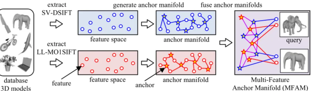
database 3D models

feature space anchor manifold  extract

LL-MO1SIFT extract SV-DSIFT

query

feature space anchor manifold  Multi-Feature Anchor Manifold (MFAM) generate anchor manifold fuse anchor manifolds

Figure 1: Our algorithm first extracts two visual features (SV-DSIFT and LL-MO1SIFT) from each 3D model. Distribution of each set of features is approximated by an anchor manifold graph. Ranking is computed by relevance diffusion on a Multi-Feature Anchor

Manifold (MFAM) produced by combining anchor manifolds of the two features.

anchor feature

3

Proposed algorithm

3.1

Overview of the algorithm

We propose 3D model retrieval by Visual Feature Fusion (3DVFF) algorithm that fuses multiple visual features of 3D models via an unsupervised distance metric fusion algorithm called Multi-Feature Anchor Manifold Ranking (MFAMR). Figure 1 shows an overview of the proposed algorithm. The 3DVFF algorithm first extracts two visual features SV-DSIFT and LL-MO1SIFT from each 3D model in a database. The SV-DSIFT aggregates local visual features extracted from multiple viewpoints by Super Vector (SV) coding [22], and shows high accuracy for models having global deformation and/or articulation. The LL-MO1SIFT aggregates per-view global image features by using Locality-constrained Linear (LL) coding [23], and shows high accuracy for rigid models. For each feature, to reduce computational cost, a manifold of all the features is approximated by a manifold of anchors. Then, the two anchor manifold graphs are fused into a MFAM graph. Ranking of the 3D models in the database for a given query is efficiently computed by relevance diffusion from the query to the 3D models over the MFAM. The two heterogeneous manifolds, one for the SV-DSIFT and the other for the LL-MO1SIFT, are fused during the relevance diffusion over the MFAM to yield a fused distance metric.

3.2

Multi-Feature Anchor Manifold Ranking

Constructing multiple anchor manifolds: Suppose {xi | i = 1, …, n} is a set of n 3D

models in a database. Each 3D model xi is represented by f different features {xi(1), …, xi(f)}.

In this paper, f = 2 since we combine two visual features, i.e., SV-DSIFT and LL-MO1SIFT. Let {ui(f) | i = 1, …, m(f)} be a set of m(f) anchors for feature f (m(f) < n). We use

k-means clustering to obtain anchors as with [11, 12].

For each feature space, we generate an n × m(f) _{sparse similarity matrix Z}(f) _which represents an anchor manifold for the feature f. Similarity between a 3D model feature xi(f)

and an anchor uj(f) is computed by using equation (1);



( ) ( )





( ) ( )



 

( ) , ( ) , 0 f f f f i j i l f l kNN i ij s s if j kNN i Z otherwise       



x u x u (1)

In the equation, s(x, y) = exp(−d(x, y)/σ) in which d(x, y) is a distance function and kNN(i) is a set of k-nearest anchors of xi. For the experiments, we use Cosine distance for d(x, y).

A set of optimal values σ(f)_{, k}(f)_{, and m}(f) _{depends on feature f.}

Fusing multiple distance metrics: Similarity matrices {Z(i)_{| i = 1, …, f} are concatenated} to generate a combined similarity matrix Z*_=[Z(1)_{, …, Z}(f)_{] which has the size of n × m}*

where m* _{is total number of the anchors. The MFAM matrix S having size m}* _{× m}* _is

generated by equation (2);

1/ 2 *T * 1/ 2

 



S D Z Z D (2)

where D is a diagonal matrix whose i-th diagonal entry is * _* 1 m

ij jZ



. The matrix S represents a similarity graph among anchors. Note that all the anchors are connected with each other in the MFAM graph. That is, anchors are linked by intra-feature similarities as well as inter-feature similarities. Diffusion of relevance on the MFAM graph S by using MR algorithm [13] produces a fused similarity from the query 3D model (a source of diffusion) to the other 3D models. We use equation (3), a formula drawn from [12] for the diffusion.

 





1

1 

 

F S I (3)

In the equation, I is an m* _{× m}* _{identity matrix and α is a regularization parameter. We}

fixed α = 0.9 for the experiments, F is a MFAM graph that embodies fused learned distance metric for multiple features. Fij is fused similarity between an anchor i and an

anchor j. Computing equation (3) is relatively inexpensive since the matrix inversion is computed on the m* _{× m}* _{matrix, a matrix much smaller than n × n matrix of the original}

MR [13].Notefurther that equations (1)-(3) can be pre-computed prior to retrieval. Ranking 3D models: Similarities among a given query 3D model and 3D models in a database can be efficiently computed by using F and Z* _{obtained in the pre-processing.} Given a query 3D model xq, two visual features, i.e., SV-DSIFT xq(1) and LL-MO1SIFT

xq(2) are first extracted from xq. Then, a similarity vectors zq(1) and zq(2) are computed by

using equation (1). zq(1) (or zq(2)) includes similarities among the feature xq(1) (or xq(2)) and

the anchors in the SV-DSIFT (or LL-MO1SIFT) feature space. zq(1) and zq(2) are

concatenated into an m*_{-dimensional vector z}

q = [zq(1), zq(2)]. Relevance diffusion among

the query xq and the 3D models in the database {xi | i = 1, …, n} is approximately

computed by equation (4);

*T

q



r z FZ (4)

in which r is an n-dimensional ranking vector in which i-th element is similarity between xq and xi. Since FZ*T can be pre-computed and zq is sparse, computing r is quite efficient.

3.3

Visual features for 3D model comparison

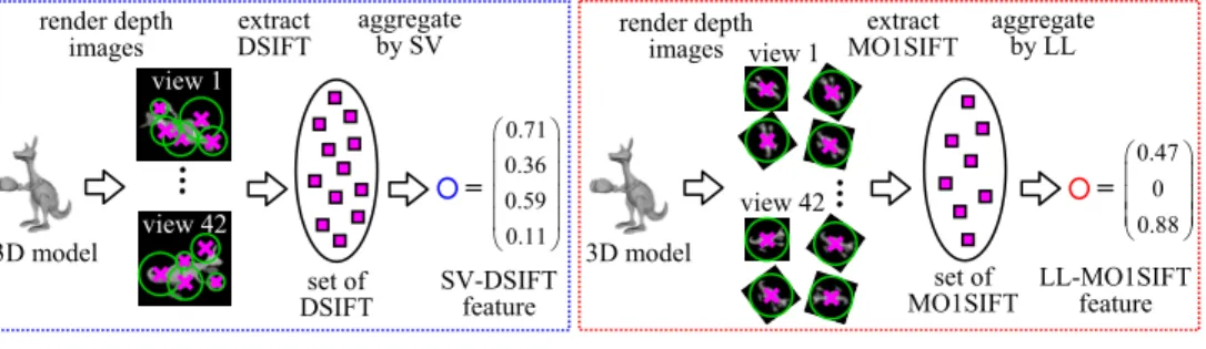
Local visual feature SV-DSIFT: The SV-DSIFT (see Figure 2(a)) is inspired by the BF-DSIFT [9] and is robust against articulation. The SV-BF-DSIFT extracts densely-sampled SIFT (DSIFT) [14] features from 42 depth-images rendered from 42 viewpoints spaced uniformly in solid angle. To render a 3D model, it is first normalized for position and scale. 42 cameras aiming at the coordinate origin are placed at vertices of a semi-regular 80-faceted polyhedron, which is generated by recursively applying Loop subdivision to an icosahedron. As about 900 DSIFT features are extracted per view, a 3D model is described by a set of about 38,000 DSIFT features. The set of 38,000 DSIFT features is aggregated by using SV coding into a feature vector per 3D model. A codebook is learned by using Gaussian Mixture Model (GMM) clustering algorithm using a set of 250,000 DSIFT features randomly selected from all the DSIFT features extracted of 3D models in the database. We use soft-assignment variant to SV coding, in which a DSIFT feature is assigned, with weights, to several neighbouring GMM centres. The weights are posterior probabilities of the DSIFT feature belonging to the assigned centres. A SV-DSIFT feature is formed by pooling weights and weighted displacements of the DSIFT features from the cluster centres. After pooling, the SV-DSIFT is normalized by its L2-norm.

SV-DSIFT is a high-dimensional feature. As the dimensionality of SIFT is 128, if the number of cluster is 2,500, dimensionality of the SV-DSIFT is (128+1)×2,500 = 322,500. To reduce the cost for constructing an anchor manifold, dimensionality of the SV-DSIFT is reduced down to d = 30~200 (d varies in benchmarks) by using Kernel PCA (KPCA).

Global visual feature LL-MO1SIFT: The LL-MO1SIFT (see Figure 2(b)) is inspired by the VM-1SIFT [8] and is sensitive to articulation. The VM-1SIFT extracts a single SIFT feature (thus 1SIFT) sampled at the centre of each of 42 multi-view rendered depth-images. Matching a pair of 3D models using VM-1SIFT is inefficient as it compares all the

422 _{=1,764 image pairs. The VM-1SIFT also lacks robustness against (in-plane) rotation of} depth-images. To improve invariance against (in-plane) rotation, we extract a set of 16 Multi-Orientation 1SIFT (MO1SIFT) features from 16 rotated images per view. For each viewpoint, the rendered image of the 3D model is in-plane rotated to 16 different orientations and a MO1SIFT feature is extracted at the centre of each oriented image. Thus a 3D model is described by a set of 42×16 = 672 MO1SIFT features. To reduce the feature matching cost, we aggregate the set of many MO1SIFT features per 3D model into a LL-MO1SIFT feature per 3D model by using LL coding. Its codebook is learned by k-means clustering of 250,000 MO1SIFT features randomly chosen from all the features computed from all the 3D models in a database. As we use a codebook having 9,000 clusters, the dimensionality of LL-MO1SIFT is 9,000. As with the SV-DSIFT, the LL-MO1SIFT feature is L2-normalized. Its dimensionality is then reduced down to d = 30~150 by using KPCA for efficient anchor manifold construction.

4

Experiments

4.1

Benchmark databases

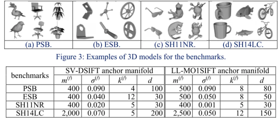
To evaluate accuracy and efficiency of the proposed 3DVFF algorithm, we use four benchmarks; the Princeton Shape Benchmark (PSB) [15], the Engineering Shape Benchmark (ESB) [16], the benchmark used for SHREC 2011 Non-Rigid watertight meshes (SH11NR) [17], and the SH14LC [18]. Figure 3 shows examples of 3D models for the benchmarks. The PSB is partitioned into a train set and a test set, each of which contains 907 generic and rigid 3D models. We use the test set having 92 semantic categories for evaluation. The ESB contains 867 CAD 3D models partitioned into 45 categories. The SH11NR consists of 600 articulated 3D models partitioned into 30 categories. The SH14LC is one of the largest benchmarks for 3DMR. It has 8,987 generic 3D models partitioned into 171 categories.

For all the benchmarks, a 3D model in the database is used as a query and remaining 3D models are used as retrieval targets. Retrieval accuracies for all the 3D models are averaged to obtain retrieval accuracy for the benchmark. We use Mean Average Precision (MAP) [%] and Discounted Cumulative Gain (DCG) [%] for quantitative evaluation of retrieval accuracy. For the SH11NR, to make visual features more robust against

render depth

images extract DSIFT aggregate by SV

set of DSIFT … SV-DSIFT feature 0.71 0.36 0.59 0.11             extract MO1SIFT aggregate by LL LL-MO1SIFT feature … view 1 view 42 0.47 0 0.88           set of MO1SIFT render depth images (b) Extracting LL-MO1SIFT. view 1 view 42

(a) Extracting SV-DSIFT.

3D model 3D model

= =

Figure 2: Extracting visual features from a 3D model. In the figure, a purple cross indicates feature location on a depth image, and a green circle indicates feature scale.

articulation, 3D models are spectrally embedded by using an algorithm by Jain and Zhang [19] prior to feature extraction. Table 1 summarizes parameters for the MFAMR algorithm.

(a) PSB. (b) ESB. (c) SH11NR. (d) SH14LC. Figure 3: Examples of 3D models for the benchmarks.

benchmarks SV-DSIFT anchor manifold LL-MO1SIFT anchor manifold m(f) _σ(f) _k(f) _{d m}(f) _σ(f) _k(f) _d

PSB 400 0.090 4 100 500 0.090 8 80

ESB 400 0.040 12 30 500 0.050 8 50

SH11NR 400 0.020 5 30 400 0.001 5 30

SH14LC 2,000 0.070 5 200 2,500 0.050 12 150

Table 1: Parameters used for MFAMR algorithm.

4.2

Retrieval accuracy of visual features

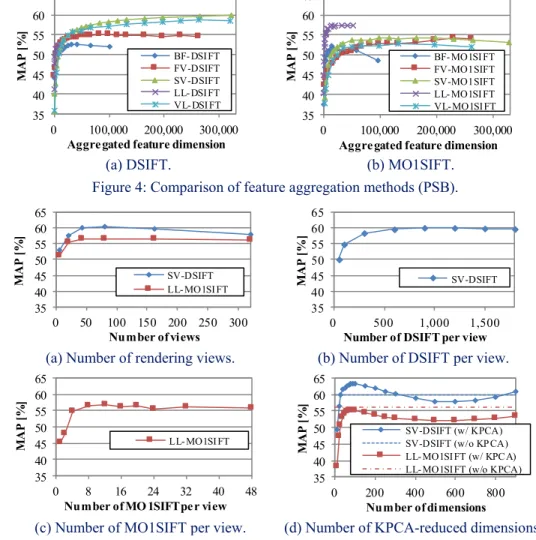
We first evaluate accuracy of our visual features under various parameter settings by using the PSB benchmark. Figure 4 shows comparison of feature aggregation methods. We compared five feature aggregation methods; BF [20], Fisher Vector (FV) [21], SV [22], LL [23], and VLAD [24]. As shown in Figure 4(a), for DSIFT, SV coding works the best. Pooling frequency of code words as well as displacements of features works well for aggregating densely-sampled local visual features. In Figure 4(b), for MO1SIFT, LL coding showed the highest accuracy. LL coding, which is one of the sparse coding methods, perform well for aggregating relatively small number of global visual features.

Figure 5(a) plots retrieval accuracy against number of viewpoints for depth-image rendering. For both SV-DSIFT and LL-MO1SIFT, 42~80 are sufficient number of viewpoints. Figure 5(b) and 5(c), for SV-DSIFT and LL-MO1SIFT, respectively, show accuracy against number of features per view. For SV-DSIFT, accuracy saturates at around 900 DSIFT features per view. For LL-MO1SIFT, 8~16 MO1SIFT features per view, that is, 8~16 rotated images per view, appears to be sufficient.

Figure 5(d) plots retrieval accuracy against dimensionality of KPCA processed feature for the PSB. For both SV-DSIFT and LL-MO1SIFT, MAP score has a peak at around 100 dimensions. As SV-DSIFT and LL-MO1SIFT features have dimensionality 322,500 and 9,000, respectively, dimension reduction by using KPCA down to 100 dimensions significantly improve computational efficiency of MFAMR algorithm.

35 40 45 50 55 60 65 0 100,000 200,000 300,000 MA P [% ]

Aggregated feature dimension

BF-DSIFT FV-DSIFT SV-DSIFT LL-DSIFT VL-DSI FT 35 40 45 50 55 60 65 0 100,000 200,000 300,000 MA P [% ]

Aggregated feature dimension

BF- MO1SI FT FV-MO1SIFT SV-MO1SIFT LL- MO1SI FT VL-MO1SIFT

(a) DSIFT. (b) MO1SIFT. Figure 4: Comparison of feature aggregation methods (PSB).

35 40 45 50 55 60 65 0 50 100 150 200 250 300 MA P [% ] Number of views SV-DSIFT LL-MO1SI FT 35 40 45 50 55 60 65 0 500 1,000 1,500 MA P [% ]

Number of DSIFT per view

SV-DSIFT

(a) Number of rendering views. (b) Number of DSIFT per view.

35 40 45 50 55 60 65 0 8 16 24 32 40 48 MA P [% ]

Number of MO 1SIFT per view

LL-MO1SI FT 35 40 45 50 55 60 65 0 200 400 600 800 MA P [% ] Number of dimensions SV-DSIFT (w/ KPCA) SV-DSIFT (w/o KPCA) LL-MO1SIFT (w/ KPC A) LL-MO1SIFT (w/o KPCA)

(c) Number of MO1SIFT per view. (d) Number of KPCA-reduced dimensions. Figure 5: Parameters and retrieval accuracy for SV-DSIFT and LL-MO1SIFT (PSB).

4.3

Effectiveness of feature fusion

In this section, we evaluate effectiveness of feature fusion using the MFAMR algorithm. We compare the MFAMR against the following six feature fusion methods;

(1) Fixed dist.: summation of Cosine distances of SV-DSIFT and LL-MO1SIFT.

(2) MR-early: ranking by MR [13] after summing Cosine distances of the two visual features. MR-early is similar to Multi-Manifold Ranking algorithm by Wang et al. [10]. (3) MR-late: MR is independently computed for SV-DSIFT and LL-MO1SIFT, and the two relevance values are summed to generate ranking. MR-late is used in [8] for 3DMR.

(4) EMR-early: MR of the method (2) is replaced with EMR [12]. (5) EMR-late: MR of the method (3) is replaced with EMR.

(6) MFAMH: hashing on MFAM [11] with 64 bits. Other parameters are same as the MFAMR.

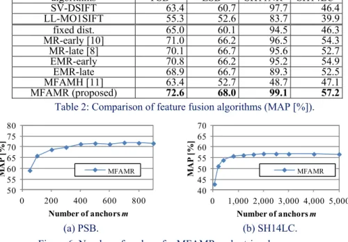
Table 2 shows retrieval accuracies of the feature fusion methods. For all the benchmarks we tested, our MFAMR showed small but consistent improvement over other fusion methods. On the other hand, the MFAMH shows inferior retrieval accuracy than other feature fusion methods. These results suggest that fusing multiple features during relevance diffusion on a MFAM is effective for improving retrieval accuracy.

Figure 6 shows plots of retrieval accuracy against the number of anchors for MFAMR. In Figure 6, the number of anchors m indicates that m anchors are used for SV-DSIFT and m anchors are used for LL-MO1SIFT. Thus the MFAM has 2m anchors. We can observe that m=400 (i.e., 800 anchors for MFAM) and m=1,000~2,000 (i.e., 2,000~4,000 anchors for MFAM) are sufficient for the PSB and the SH14LC, respectively. With smaller number of anchors, retrieval accuracy declines since the MFAMR fails to approximate structure of the original multi-feature manifold.

algorithms PSB ESB SH11NR SH14LC SV-DSIFT 63.4 60.7 97.7 46.4 LL-MO1SIFT 55.3 52.6 83.7 39.9 fixed dist. 65.0 60.1 94.5 46.3 MR-early [10] 71.0 66.2 96.5 54.3 MR-late [8] 70.1 66.7 95.6 52.7 EMR-early 70.8 66.2 95.2 54.9 EMR-late 68.9 66.7 89.3 52.5 MFAMH [11] 63.4 52.7 48.7 47.1 MFAMR (proposed) 72.6 68.0 99.1 57.2

Table 2: Comparison of feature fusion algorithms (MAP [%]).

50 55 60 65 70 75 80 0 200 400 600 800 MA P [% ] Number of anchors m MFAMR 40 45 50 55 60 65 70 0 1,000 2,000 3,000 4,000 5,000 MA P [% ] Number of anchors m MFAMR (a) PSB. (b) SH14LC. Figure 6: Number of anchors for MFAMR and retrieval accuracy.

4.4

Efficiency

Table 3 shows computation time per query. In table 3, columns “SV-DSIFT” and “LL-MO1SIFT” are times for extracting SV-DSIFT and LL-MO1SIFT from a query 3D model. “Ranking” is a time for computing relevance among the query and 3D models in a database. For interactive retrieval, feature extraction is accelerated by using a GPU and multi-core CPUs. MR computation for the MR-early is accelerated by using a GPU. MFAMR is computed on a CPU with single thread. We used a PC having two Intel Xeon E5-2650V2 CPUs, 256GB DRAM, and an Nvidia GeForce 770 GPU with 4GB of memory.

As shown in Table 3, the MFAMR takes less than 3 seconds per query for both the PSB and the SH14LC. In contrast, retrieval by MR-early for the SH14LC takes more than 30 seconds per query due to costly inversion of a large similarity matrix.

benchmarks algorithms SV-DSIFT LL-MO1SIFT Ranking total PSB

(907 models) MR-earlyMFAMR 2.0762.076 0.4960.496 0.0020.548 2.574 3.120 SH14LC

(8,987 models) MR-earlyMFAMR 2.0792.079 0.4960.496 34.7790.031 37.354 2.606

Table 3: Computation time per query [s].

4.5

Comparison with other algorithms

Table 4 compares retrieval accuracy of the proposed 3DVFF algorithm with other state-of-the-art 3D model retrieval algorithms. For all the four benchmarks, our proposed 3DVFF algorithm achieved the highest retrieval accuracy among the algorithms listed in Table 4. For the SH14LC benchmark, MAP score of our 3DVFF is 3% higher than LCDR-DBSVC, the best performing algorithm among the SH14LC track entries [18]. In addition to being more accurate, our 3DVFF is also much faster than LCDR-DBSVC, which performs MR for each query. Figure 7 shows two queries and their retrieval results for 3DVFF and MR-D1SIFT [8], latter of which finished 2nd in the SH14LC track.

algorithms _{DCG MAP DCG MAP DCG MAP DCG MAP} PSB ESB SH11NR SH14LC

LFD [3] 64.3 40.7 72.9 43.8 73.9 43.4 71.7 31.7 BF-DSIFT [9] 71.6 50.4 78.0 52.5 91.6 77.3 75.3 37.5 VM-1SIFT [8] 69.7 48.4 76.2 49.0 72.0 39.2 68.8 26.9 MR-D1SIFT [8] 78.7 62.9 81.5 59.2 94.2 83.9 79.2 46.4 HSR-DE [4] 69.9 81.3 75.2 37.8 SD-GDM-meshSIFT [17] 99.6 LCDR-DBSVC [18] 82.3 54.1 SV-DSIFT 80.2 63.4 82.5 60.7 99.3 97.7 80.2 46.4 LL-MO1SIFT 74.7 55.3 78.9 52.6 93.7 83.7 76.1 39.9 3DVFF (proposed) 84.1 72.6 85.1 68.0 99.7 99.1 83.7 57.2

Table 4: Comparison of retrieval accuracy [%].

(a) MR-D1SIFT.

(b) 3DVFF (proposed).

Figure 7: Examples of retrieval results for the SH14LC. Our 3DVFF algorithm produces better results than MR-D1SIFT [8] which is a 2nd place finisher for the SH14LC [18].

query

query query

5

Conclusion

In this paper, we proposed a 3D model retrieval algorithm called 3D model retrieval by Visual Feature Fusion (3DVFF) that fuses multiple visual features for effective and efficient retrieval. For efficiency, we employ Multi-Feature Anchor Manifold (MFAM) that approximates multiple manifolds of features by using small number of “anchor” features. Ranking of 3D models for a query is performed by relevance diffusion on the MFAM. Distance metrics for heterogeneous features are fused during relevance diffusion via cross-linking of manifolds. For better “raw” visual feature similarities, we employed state-of-the-art feature aggregation methods, i.e., Super Vector coding [22] and Locality-constrained Linear coding [23]. Experiments show that our proposed algorithm is more accurate and much faster than state-of-the-art 3DMR algorithms we have compared against.

Acknowledgement

This research is supported by JSPS Grant-in-Aid for Scientific Research on Innovative Areas #26120517 and JSPS Grants-in-Aid for Scientific Research (C) #26330133.

References

[1] J. W. H. Tangelder and R. C. Veltkamp. A survey of content based 3D shape retrieval methods, Multimedia Tools and Applications, 39(3):441-471, 2008.

[2] B. Li, A. Godil, M. Aono, X. Bai, T. Furuya, L. Li, R. Lopez-Sastre, H. Johan, R. Ohbuchi, C. Redondo-Cabrera, A. Tatsuma, T. Yanagimachi, and S. Zhang. SHREC'12 Track: Generic 3D Shape Retrieval, Proc. EG 3DOR 2012, 2012.

[3] D-Y. Chen, X.-P. Tian, Y-T. Shen, and M. Ouh-young. On Visual Similarity Based 3D Model Retrieval, Computer Graphics Forum, 22(3):223–232, 2003.

[4] M. Aono, H. Koyanagi, and A. Tatsuma. 3D shape retrieval focused on holes and surface roughness, Proc.APSIPA2013, 2013.

[5] B. Li and H. Johan. 3D model retrieval using hybrid features and class information, Multimedia

Tools and Applications, 62(3): 821–846, 2013.

[6] A. Tatsuma and M. Aono. Multi-Fourier spectra descriptor and augmentation with spectral clustering for 3D shape retrieval, The Visual Computer, 25(8):785–804, 2009.

[7] P. Papadakis, I. Pratikakis, T. Theoharis, G. Passalis, and S. Perantonis. 3D Object Retrieval using an Efficient and Compact Hybrid Shape Descriptor, Proc.EG 3DOR 2008:9–16, 2008. [8] R. Ohbuchi and T. Furuya. Distance metric learning and feature combination for shape-based

3D model retrieval, Proc. 3DOR2010:63–68, 2010.

[9] T. Furuya and R. Ohbuchi. Dense sampling and fast encoding for 3D model retrieval using bag-of-visual features, Proc. ACM CIVR 2009, Article No. 26, 2009.

[10] Y. Wang, M. A. Cheema, X. Lin, and Q. Zhang. Multi-Manifold Ranking: Using Multiple Features for Better Image Retrieval, AKDDM, 7819:449–460, 2013.

[11] S. Kim and S. Choi. Multi-view anchor graph hashing, Proc. ICASSP2013:3123–3127, 2013. [12] B. Xu, J. Bu, C. Chen, D. Cai, X. He, W. Liu, and J. Lu. Efficient Manifold Ranking for Image

[13] D. Zhou, J. Weston, A. Gretton, O. Bousquet, and B. Schölkopf. Ranking on Data Manifolds,

Proc. NIPS2004, 2004.

[14] D. G. Lowe. Distinctive Image Features from Scale-Invariant Keypoints, IJCV, 60(2):91–110, 2004.

[15] P. Shilane, P. Min, M. Kazhdan, and T. Funkhouser. The Princeton Shape Benchmark, Proc.

SMI 2004:167–178, 2004. http://shape.cs.princeton.edu/

[16] S. Jayanti, Y. Kalyanaraman, N. Iyer, and K. Ramani. Developing an engineering shape benchmark for CAD models, Proc CAD, 38(9):939–953, 2006.

[17] Z. Lian, A. Godil, B. Bustos, M. Daoudi, J. Hermans, S. Kawamura, Y. Kurita, G. Lavoué, H.V. Nguyen, R. Ohbuchi, Y. Ohkita, Y. Ohishi, F. Porikli, M. Reuter, I. Sipiran, D. Smeets, P. Suetens, H. Tabia, and D. Vandermeulen. SHREC'11 Track: Shape Retrieval on Non-rigid 3D Watertight Meshes, Proc. EG 3DOR 2011:79–88, 2011.

[18] B. Li, Y. Lu, C. Li, A. Godil, T. Schreck, M. Aono, Q. Chen, N. K. Chowdhury, B. Fang, T. Furuya, H. Johan, R. Kosaka, H. Koyanagi, R. Ohbuchi, and A. Tatsuma. Large Scale Comprehensive 3D Shape Retrieval, Proc. EG 3DOR 2014:131–140, 2014.

[19] V. Jain and H. Zhang. Robust 3D Shape Correspondence in the Spectral Domain, Proc. SMI 2006, 2006.

[20] G. Csurka, C.R. Dance, L. Fan, J. Willamowski, and C. Bray. Visual Categorization with Bags of Keypoints, Proc. ECCV 2004 workshop on Statistical Learning in Computer Vision:59–74, 2004.

[21] F. Perronnin and C. Dance. Fisher kernels on visual vocabularies for image categorization,

Proc. CVPR 2007, 2007.

[22] X. Zhou, K. Yu, T. Zhang, and T.S. Huang. Image Classification using Super-Vector Coding of Local Image Descriptors, Proc. ECCV 2010:141–154, 2010.

[23] J. Wang, J. Yang, K. Yu, F. Lv, T. Huang, and Y. Gong. Locality-constrained Linear Coding for Image Classification, Proc. CVPR 2010:3360–3367, 2010.

[24] H. Jegou, M. Douze, C. Schmid, and P. Perez. Aggregating local descriptors into a compact image representation, Proc. CVPR 2010:3304–3311, 2010.

[25] G. K.L. Tam and R. Lau. Embedding Retrieval of Articulated Geometry Models, IEEE Trans.