Topological Data Analysis for Clustering and Classifying Time Series

(1)

OpenCommons@UConn

Doctoral Dissertations University of Connecticut Graduate School 12-2-2019

Topological Data Analysis for Clustering and Classifying Time

Series

Renjie Chen

University of Connecticut - Storrs, [email protected]

Follow this and additional works at: https://opencommons.uconn.edu/dissertations

Recommended Citation Recommended Citation

Chen, Renjie, "Topological Data Analysis for Clustering and Classifying Time Series" (2019). Doctoral Dissertations. 2365.

(2)

Classifying Time Series

Renjie Chen, PhD

University of Connecticut, 2019

ABSTRACT

Topological Data Analysis (TDA), which refers to methods of utilizing topological features in data (such as connected components, tunnels, voids, etc.) has gained consid-erable momentum. More recently, TDA has been increasingly used for analyzing time series. The recent researches of using TDA in time series are mainly focused on un-supervised and un-supervised learning. In this thesis, a review of TDA will be provided, following by using TDA in time series for doing unsupervised and supervised learning for different applications.

(3)

Classifying Time Series

Renjie Chen

BS, University of Science and Technology Beijing, 2014

A Dissertation

Submitted in Partial Fulfillment of the Requirements for the Degree of

Doctor of Philosophy at the

University of Connecticut 2019

(4)

Copyright by

Renjie Chen

(5)

APPROVAL PAGE

Doctor of Philosophy Dissertation

Topological Data Analysis for Clustering and Classifying Time

Series

Presented by

Renjie Chen, B.S. Applied Mathematics

Major Advisor Nalini Ravishanker Associate Advisor Haim Bar Associate Advisor Zhiyi Chi University of Connecticut 2019

(6)

Acknowledgements

When I started in this doctoral program, I was only thinking of it as a way for me to enjoy school life more before entering into the industry. I thought it was simply a diploma with a couple more years on campus. Turns out this is simply naive. I can never imagine it enhances me a lot of analytic and writing skills, and let me realize that doing research is such a serious, pure, sacred and beautiful thing. Though I am not making fundamental contributions to the scientific field, the achievements I can make, as well as significant personal developments, are attributed to the support and selfless help of my mentor and the entire department and colleagues.

Without my advisor, I cannot finish this Ph.D. Without the selfless supports of my department, I think I probably already go back home doing something boring and live like a livestock. There are too many people to thank, like department head, program assistant, and I may not put down their names. Last but not least, I am lucky of being here, making stupid mistakes and making improvements.

(7)

List of Tables

1 Pairwise Bottleneck Distances Between Persistence Diagrams for Different

d. . . 34 2 Data Sources and Sample Sizes . . . 81 3 Total Weights of Different Demographic Variables . . . 83 4 Model Comparisons for Choosing Number of Clusters K: The number of

clusters; WCSS; CPU Time seconds (feature extraction + K-means). . . 86 5 The 95% percentile of the nominal empirical distribution and the powers.

The “1 vs 2” meansk1 = 1, k2 = 2. . . 108 6 Comparisons of Average Accuracy of Clustering. Different PL orders

Corresponding to Three SNR Values. . . 129 7 Average accuracy using different dissimilarity matrix constructions. . . . 150

(12)

List of Figures

1 Topology of three objects in the topological space. . . 11

2 The examples of two objects in the topological space. . . 14

3 Matrix operations of the Object one. . . 16

4 Matrix operations of the Object two. . . 17

5 Persistence diagram corresponding to a point cloud. (a) shows the raw point cloud and (h) shows the persistence diagram. (c), (e) and (g) are intermediate steps for the filtration by varying λ, while (b), (d) and (f) are intermediate steps for constructing the persistence diagram. . . 27

6 Pure Periodic Signals to Persistence Diagrams. . . 34

7 Persistence Diagrams of Periodic Time Series with Different Shapes . . . 39

8 Construction of a persistence diagram corresponding to a one-dimensional continuous real function. (a) is the function and (h) is the persistence diagram. (c), (e) and (g) show the sublevel set filtration procedure, while (b), (d) and (f) are the intermediate steps for constructing the persistence diagram. . . 43

9 Distance-to-Measure (DTM) function and the persistence diagram. . . . 46

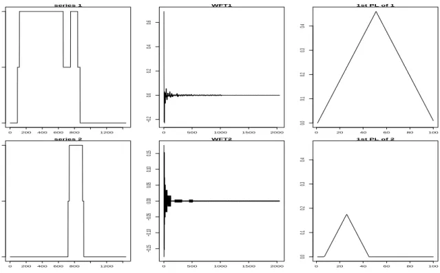
10 Persistence diagrams using second-order spectrum. . . 48

(13)

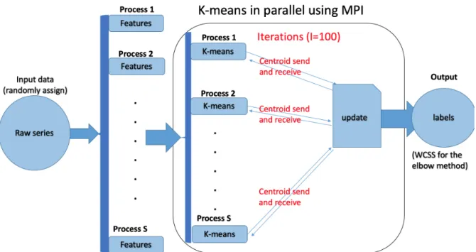
12 Persistence landscapes of the persistence diagram pers.diag.3. . . 55 13 Persistence diagrams using Walsh-Fourier Transforms. . . 59 14 An Overview of Implementing the Divide and Combine Scheme. . . 79 15 Time Course Proportions of the Three Categories for the Five Survey

Waves. . . 84 16 Categorical Time Series for Randomly Selected Respondents. . . 85 17 WCSS versus Number of ClustersK. . . 86 18 Three clusters proportions. The x-axis is the minutes and the y-axis is

the proportion of three categories: Blue-Home, Red-Travel, Green-Out of Home. The title gives the name of the cluster and the size of it. “C1-in home: 115530” means that the first proportion plot is the cluster one, called “in home” cluster, and there are total 115530 adults in C1. . . 88 19 The composition of different clusters over five survey periods, as a function

of five different generations. . . 89 20 The composition of different clusters over five surveys periods, as a

func-tion of gender. . . 90 21 The composition of different clusters over five surveys periods, as a

func-tion of worker/non-workers. . . 91 22 The composition of different clusters over five survey periods, as a function

(14)

23 Four pairs of plots, in order from top left to bottom right, to illustrate the procedure of getting the persistence diagram on a function . . . 97 24 Three clusters proportions. Blue, Red and Green are three categories of

the time series. . . 100 25 The empirical distributions of statisticsLC(k1, k2) =

PN

t=1(ck1,t−µk2,t)

N over

1000 samples. . . 102 26 Three clusters proportions by using the first-order persistence landscape. 112 27 The Home category of three clusters on different methods. . . 113 28 Persistence Diagram for Example 1. . . 121 29 Persistence Landscapes for Example 1. . . 122 30 Raw Temperatures (blue) and Detrended Temperatures (black) from Four

Locations. . . 130 31 Persistence Landscape (PL) Order Selection Using the Elbow Method for

Time Series of Temperatures. . . 131 32 Selecting the Number of Clusters Using the Average Silhouette Method. . 131 33 Persistence landscapes of the persistence diagram. . . 132 34 Distribution of locations in three clusters. . . 134 35 Two objects in the topological space with different topological structures. 141 36 Simulated Time Series from Scenario one. . . 149 37 Segmentation selection using first homology classes. . . 150 38 P-waves for the Earthquake-Explosion Time Series . . . 152

(15)

39 S-waves for the Earthquake-Explosion Time Series . . . 152

40 Segmentation selection using first homology classes. . . 154

41 Feature scores using P-waves and S-waves on different methods. . . 155

42 Nine cases of the Eigenworm time series. . . 156

43 Segmentation selection using first homology classes. . . 158 44 Variable importance plot using feature scores for the random forest classifier.159

(16)

Chapter 1 Introduction

Developing useful algorithms for feature construction that enable learning about a large number of time series is an important area with applications in several domains. This is especially the case in recent years with the increasing availability of large numbers of long and complex time series data. The constructed features can then be used in classification or clustering the time series, among other things. Aghabozorgi et al. (2015) categorized feature representations for time series into four broad types: (i) data adaptive represen-tations, useful for time series of arbitrary lengths; (ii) non-data adaptive approaches, used for time series of fixed lengths; (iii) model based methods, used for representing time series in a stochastic modeling framework; and (iv) data dictated approaches, which are automatically defined based on raw time series.

One recently emerging approach is the use of Topological Data Analysis (TDA) for analyzing complex data. TDA refers to a class of methods that garner information from topological structures in data that belong to a topological space, i.e., a mathematical space that allows for continuity, connectedness, and convergence (Carlsson, 2009; Edels-brunner and Harer, 2010). Output from TDA has been used for effective statistical

(17)

learning about the data. Thus, TDA combines algebraic topology and other tools from pure mathematics to allow a useful study ofshape of the data. The most widely discussed topologies of data include connected components, tunnels, voids, etc., of a topological space. Computational (or algorithmic) topology, is an overlap between the mathemat-ical underpinnings of topology with computer science, and consists of two parts, i.e., measuring the topology of a space and persistent homology (Chazal and Michel, 2017). Using computational topology, TDA aims at analyzing topological features of data and representing these features using low dimensional representations (Carlsson, 2009). Per-sistent homology refers to a class of methods for measuring topological features of shapes and functions. It converts the data into simplicial complexes and describes the topo-logical structure of a space at different spatial resolutions. Topologies that are more persistent are detected over a wide range of spatial scales and are deemed more likely to represent true features of the underlying space rather than sampling variations, noise, etc. Persistent homology therefore elicits persistence of essential topologies in the data and outputs the birth and death of such topologies via a persistence diagram, which is a popular summary statistic in TDA.

Development of TDA for time series is a relatively new area, with many interesting applications in several different domains. This is the topic of investigation in this the-sis. Berwald et al. (2013) discussed the use of TDA in climate analythe-sis. Khasawneh and Munch (2016) used notions of persistence of first homology groups of point clouds (obtained via Takens’s embedding) within multiple windows of time series to track the

(18)

stability of dynamical systems, while Seversky et al. (2016) explored stability of various single-source and multi-source signals. Perea and Harer (2015) used the notion of maxi-mum persistence of homology groups to quantify periodicity of time series. Pereira and de Mello (2015) used features derived from persistent homology to cluster populations of Tribolium flour beetles. Umeda (2017) used topological features of one and two dimen-sional homology groups as inputs into convolutional neural networks for classification of time series in three different domains, showing that their approach outperformed the baseline algorithm in each case. One illustration consisted of motion sensor data of daily and sports activities, an area also investigated using TDA by Stolz et al. (2017). Truong (2017) as well as Gidea (2017); Gidea and Katz (2018) and Gidea et al. (2018) explored the use of TDA on financial time series.

This thesis describes using TDA for constructing features of time series and uses these for clustering and classification. The thesis has five chapters. Chapter 2 introduces TDA by explaining mathematical terminologies with examples, followed by a detailed review of TDA for time series analysis. Chapter 3 describes our work on using TDA to understand activity-travel behavior over one day of survey respondents in a very large, multi-wave study. We employ first order persistence landscapes of the time series along with a divide-and-combine scheme and the k-means algorithm to cluster a large number of categorical time series (Chen et al., 2019). Chapter 4 discusses an approach for selecting a suitable order of the persistence landscapes, between using a first order landscape and using all orders (i.e., a very large number). We illustrate this for clustering

(19)

time series of daily temperatures at multiple locations in the US. Chapter 5 discusses the use of persistence diagrams for classifying very long time series and illustrates on a data set on the motion of worms.

(20)

Chapter 2 A Survey of Topological Data

Analysis (TDA) for Time Series

The study of topology is strictly speaking, a topic in pure mathematics. However in only a few years, Topological Data Analysis (TDA), which refers to methods of utilizing topological features in data (such as connected components, tunnels, voids, etc.) has gained considerable momentum. More recently, TDA is being used to understand time series. This article provides a review of TDA for time series, with examples using R functions. Features derived from TDA are useful in classification and clustering of time series and in detecting breaks in patterns.

2.1 Introduction

Topological Data Analysis (TDA) is now an emerging area for analyzing complex data. TDA refers to a class of methods that garner information from topological structures in data that belong to a topological space, i.e., a set X together with a collection of subsets of X, namely ℵ, such that the empty set φ and the whole set X are open sets

(21)

(i.e. any sets belonging to ℵ are called open sets), and such that arbitrary unions and finite intersections of open sets are still open sets (Carlsson, 2009; Edelsbrunner and Harer, 2010; Munkres, 1993). Output from TDA may then be used for effective statis-tical learning about the data. TDA combines algebraic topology and other tools from pure mathematics to allow a useful study of shape of the data. The most widely dis-cussed topologies of data include connected components, tunnels, voids of a topological space. Computational (or algorithmic) topology, is an overlap between the mathemat-ical underpinnings of topology with computer science, and consists of two parts, i.e., measuring the topology of a space and persistent homology (Chazal and Michel, 2017). Using computational topology, TDA aims at analyzing topological features of data and representing these features using low dimensional representations (Carlsson, 2009). In particular, the space must first be represented as simplicial complexes (the defintion and details will be provided in subsection 2.2.1), the Vietoris-Rips complex and the

ˇ

Cech complex being the most common pathways to obtaining output to characterize the topology.

Persistent homology refers to a class of methods for measuring topological features of shapes and functions. It converts the data into simplicial complexes and describes the topological structure of a space at different spatial resolutions. Topologies that are more persistent are detected over a wide range of spatial scales and are deemed more likely to represent true features of the underlying space rather than sampling variations, noise, etc. Persistent homology therefore elicits persistence of essential topologies in the data

(22)

and outputs the birth and death of such topologies via a persistence diagram, which is a popular summary statistic in TDA. Data inputs for persistent homology are usually represented as point clouds or as functions, while the outputs depend on the nature of the analysis and commonly consist of either a persistence diagram, or a persistence landscape. A point cloud of data represents a sample of points from an underlying manifold and its persistent homology approximates the topological information of the manifold. If data is represented as a Morse function (i.e., a smooth function on the manifold such that all critical points are non-degenerate), the persistent homology of the function is mathematically equivalent to analyzing the topological information of the manifold. For rigorous expositions on algebraic topology and computational homology, see Munkres (1993) and Edelsbrunner and Harer (2010).

TDA has been used in cosmic web (van de Weygaert et al., 2013), shape analysis (Carlsson et al., 2004; Chazal et al., 2009; Di Fabio and Landi, 2011; Fabio and Landi, 2012; Chazal et al., 2014; Li et al., 2014; Carri`ere et al., 2015; Bonis et al., 2016), biological data analysis (DeWoskin et al., 2010; Nicolau et al., 2011; Heo et al., 2012; Kovacev-Nikolic et al., 2016; Bendich et al., 2016; Wang et al., 2018), sensor networks (Silva and Ghrist, 2007; De Silva and Ghrist, 2007; Adams and Carlsson, 2015), as well as other fields.

Development of TDA for time series is a relatively new and fast growing area, with many interesting applications in several different domains. Berwald et al. (2013) dis-cussed the use of TDA in climate analysis. Khasawneh and Munch (2016) used notions

(23)

of persistence of first homology groups of point clouds (obtained via Takens’s embed-ding) within multiple windows of time series to track the stability of dynamical systems, while Seversky et al. (2016) explored stability of various single-source and multi-source signals. Perea and Harer (2015) used the notion of maximum persistence of homology groups to quantify periodicity of time series. Pereira and de Mello (2015) used fea-tures derived from persistent homology to cluster populations of Tribolium flour beetles. Umeda (2017) used topological features of one and two dimensional homology groups as inputs into convolutional neural networks for classification of time series in three differ-ent domains, showing that their approach outperformed the baseline algorithm in each case. One illustration consisted of motion sensor data of daily and sports activities, an area also investigated using TDA by Stolz et al. (2017). Truong (2017) as well as Gidea (2017); Gidea and Katz (2018) and Gidea et al. (2018) explored the use of TDA on financial time series. We discuss some of these applications in detail later in this paper. According to Fulcher and Jones (2014); Aghabozorgi et al. (2015), it is not nature to represent time series as a point cloud. The transformation from a time series to a point cloud is implemented through Takens’s embedding (Takens et al., 1981), preserving the underlying manifold of the time series. The approach consists of transforming a time series {xt, t = 1,2, . . . , T}, into its phase space, i.e., a point cloud or a set of points

vi = {xi, xi+τ, . . . , xi+dτ}, i = 1,2, . . . , T − dτ, where τ is a delay parameter and d

specifies the dimension of the point cloud. We discuss Takens’s embedding in Section 2.3.3 and the selection ofd and τ in Section 2.3.3. TDA of time series through suitable

(24)

functions is much less explored. Wang et al. (2018) proposed TDA on weighted Fourier series representations (Morse functions) of electroencephalogram (EEG) data. They used a randomness test approach to examine properties of the proposed method and show its robustness to different transformations of the data. TDA of time series through sublevel set filtration of functions is discussed in Section 2.4.

The format of this chapter follows. Section 2.2 gives a review of the mathematical terminologies and computations with examples. Section 2.3 provides a review of TDA from point clouds and then describes TDA for time series via the Takens’s embedding method. Section 2.4 provides a review of persistent homology on functions and then describes TDA for time series analysis starting from second-order spectra or Walsh Fourier transforms. Section 2.5 discusses constructing TDA based features which are then used in learning about time series, with applications on classification, clustering and detecting changes in patterns. Section 3.5 gives a discussion and summary.

2.2 Mathematical Preliminaries of TDA

2.2.1 Homology Equivalence

Homology is used to summarize the connectivity of a topological spaceS and to detect holes in S. In algebraic topology, the ˜p-th homology group Hp˜(S) is the quotient of

the kernel of the ˜p-th simplicial complex group to the image of the (˜p+ 1)-th simplicial complex group (Spanier, 1989). The rank of Hp˜(S) is the ˜p-th Betti number ˜βp˜(S). In

(25)

other words, the ˜p-th Betti number ˜βp˜(S) counts the number of ˜p dimensional holes in

the space S. The 0-th Betti number, ˜β0, denotes the number of connected components

in the topological space S, the first Betti number ˜β1 denotes the number of loops in S,

the second Betti number ˜β2 denotes the number of the enclosed void spaces in S, and

so on.

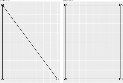
We use Figure 1 as an example to introduce the topology of objects in the topological space. From left to right, the first object S1 has only one ( ˜β0(S1) = 1) connected

component, as all the points of the object are connected to each other. There is also one ( ˜β1(S1) = 1) cycle in the object. The second objectS2 has two ( ˜β0(S2) = 2) connected

components as there is one separate point from the cycle. There is one ( ˜β1(S2) =

1) cycle enclosing the empty space. The third object S3 has only one ( ˜β0(S3) = 1)

connected component as all points of the object are connected. However, there are three ( ˜β1(S3) = 3) cycles of the object as there are three separate empty areas enclosed

by the connected component. Topological computations are done by representing the objects as simplicial complexes; the classical simplicial complexes used often are called Vietoris-Rips complexes.

Homology of Abstract Simplicial Complexes. In order to calculate the Betti numbers, there are some definitions to walk through. Suppose there are a set of (n+ 1) distinct points o = {o0, o1, o2, . . . , on} ⊂ Rd in the space. The ˜p-dimensional simplice κp˜ =

[o0, o1, o2, . . . , op˜] spanned by o is the convex hull of o. The points in o are called the

(26)

Figure 1: Topology of three objects in the topological space. of κp˜.

A geometric simplicial complex ˜˜κ in Rd _{is defined as a collection of simplices such}

that:

• Any face of a simplice of ˜˜κis a simplice of it: ∀κ2 ∈κ,˜˜ ∀κ1 is a face ofκ2 ⇒κ1 ∈κ˜˜

• The intersection of any two simplices of ˜˜κ is empty or a common face of both:

∀κ1, κ2 ∈κ,˜˜ ⇒κ1∩κ2 is a face of both of κ1 and κ2 or empty.

The geometric simplicial complexes are particularly useful for TDA as they are used to form the abstract simplicial complexes, which are used to measure the topology. Partic-ularly, the geometric simplicial complexes builds the connection between the practical dataset and topology.

Using a geometric simplicial complex, an abstract simplicial complex ˜κ is defined by a nonempty set ˜o of elements, denoting the vertices:

(27)

• ∀κ1 ∈κ,˜ ∀κ2 ⊂κ1 ⇒κ2 ∈κ˜

For example, if ˜o = {o˜1,o˜2}, then there are three abstract simplicial complexes:

[õ1] = {õ1},[õ2] = {o˜2}, [õ1,õ2] = {o˜1,o˜2,(õ1,o˜2)}. Intuitively, the abstract simplicial

complex ˜κ is a combination of the geometric simplicial complex ˜κ˜ and it assumes the vertices to be set in the more general space, namely the topological spaceS. Specifically, ˜

˜

κ is a geometric realization of ˜κ, which means that embedding ˜κ˜ into ˜κ is an injective mapping. In this way, the ˜κ(used for topological features) is used as the representation of ˜κ (the data).

Let ˜κK be a K-dimensional abstract simplicial complex with the nonempty set ˜o of

size K. A ˜p-chain is defined as a formal sum of ˜p-simplices in ˜κK, ˜C=Pδ˜iκi, whereκi

is a ˜pdimensional simplice in ˜κK and ˜δi is the coefficient, which can only be 0 or 1. For

example, 1×κ1 + 1×κ1 = 0×κ1 = 0. Combining all ˜p-chains with the sum operator

gives a group of ˜p-chains, ˜Cp˜(˜κ). Further, we define the boundary of a ˜p- dimensional

simplice κ as the sum of all its (˜p−1) dimensional faces, denotes as ˜∂κ =P

κi, κi are

all faces of κ.

It is sufficient to calculate topologies from the ˜κ, which are Betti numbers. The kernel of the ˜p-th simplicial complex group, ˜Zp˜(˜κ), is a subgroup of the ˜Cp˜(˜κ): ∀ C˜ ∈

˜

Zp˜(˜κ),∂˜C˜ = 0. Denote ˜Z0(˜κ) = ˜C0(˜κ). The image of (˜p+1)-th simplicial complex group,

˜

Bp˜(˜κ), is also a subgroup of ˜Cp(˜κ) since ˜Bp˜(˜κ) = ˜∂C˜p˜+1(˜κ) ( ˜∂C˜p˜+1(˜κ) means taking the

boundary ˜∂ on each (˜p+ 1)-chains of ˜Cp˜+1(˜κ)). To show it as a subgroup of ˜Cp(˜κ): ∀ κ

(28)

˜

∂P˜

δiκi =

P˜

δi∂κ˜ i, which is a ˜p-chain ∈C˜p˜(˜κ). In fact, ˜Bp˜(˜κ) ⊂ Z˜p(˜κ) because of the

fact that ∀p˜-chain c,∂˜( ˜∂c) = 0.

Finally, the ˜p-th homology group is Hp˜(˜κ) = ˜Zp˜(˜κ)/B˜p˜(˜κ) = {c + ˜Bp˜(˜κ),∀ c ∈

˜

Zp˜(˜κ)} with the sum operator. The Betti number ˜βp˜(˜κ) = rank ofHp˜(˜κ). For example,

˜

κ = {o1, o2,(o1, o2)}, then for the elements of the groups, ˜Z0(˜κ) = ˜C0(˜κ) : {o1, o2, o1 +

o2},B˜0(˜κ) = ˜∂C˜1(˜κ) : ˜∂{(o1, o2)} = {o1 +o2} ⇒ Hp˜(˜κ) : {c+ ˜Bp˜(˜κ),∀c ∈ Z˜p˜(˜κ)} =

{o1 + ˜Bp˜(˜κ)} because {o1 + ˜Bp˜(˜κ)} = {o1 + (o1 +o2), o1 + (o1 +o2) + (o1 +o2)} =

{o2 + ˜Bp˜(˜κ)}={o1, o2} and {o1+o2+ ˜Bp˜(˜κ)}={o1+o2, φ}, which means the 0-chain

{o1 +o2} and the empty set are homologous but we are only interested in any ˜p-chains

non-homologous to the empty set. Therefore, ˜β0(˜κ) =rank of H0(˜κ) = 1. And ˜Z1(˜κ) is

empty as the only 1-dimensional simplicec= ˜δ(o1, o2), ˜∂c= ˜δ∂˜(o1, o2) = ˜δ(o1+o2)6= 0.

We use two examples in Figure 2 to introduce the computation. The topologies are called the homology classes, {α˜p,k˜ ,p˜= 0,1;k = 1,2, . . . kp˜}. Specifically, {α˜0,k, k =

1,2, . . . , k0} are the connected components and {α˜1,k, k = 1,2, . . . , k1} are the tunnels

in the topological space. The Vietoris-Rips complexes consist of a set with 0,1 and 2-dimensional simplices. Specifically, the Vietoris-Rips complexes of ,object one S1, in

Figure 2 are defined as the set [A, B, C] = {A, B, C,(A, B),(A, C),(B, C),(A, B, C)}, where A, B, C are three elements of the object, (A, B),(A, C),(B, C) are three edges and (A, B, C) is the area inside of the A, B, C. In object one, the boundary group

˜

B1([A, B, C]) = ({[A, B]+[B, C]+[A, C]}|+), where [A, B] ={A, B,(A, B)}, and|{A}|+

(29)

A B C Object 1 A B C D Object 2

Figure 2: The examples of two objects in the topological space.

operation + is a binary operation, meaning [A, B]+[A, B] =φ. Further, ˜B0([A, B, C]) =

({∂˜[A, B],∂˜[B, C],∂˜[A, C]}|+) = ({[A] + [B],[B] + [C],[A] + [C]}|+). The boundary operation can be taken multiple times. ˜∂ ∂˜([A, B, C]) = ˜∂[A, B] + ˜∂[B, C] + ˜∂[A, C] = ([A] + [B]) + ([B] + [C]) + ([A] + [C]) =φ. Specifically, the ˜∂[A], ˜∂[B] and ˜∂[C] all equal to φ. The kernel groups of object one are elements giving φ when taking the boundary operation, namely ∀˜c ∈ Z˜p˜([A, B, C]),∂˜˜c = φ. Thus, the kernel groups ˜Zp˜([A, B, C])

of the object one are ˜Z1([A, B, C]) = ({[A, B] + [B, C] + [A, C]}|+), ˜Z0([A, B, C]) =

(30)

The homology classes can now be computed as ˜ Z0([A, B, C])/B˜0([A, B, C]) = ({c˜+ ˜B0([A, B, C]),˜c∈Z˜0([A, B, C])}|+) (2.1) = ([A] + [B] + [C]|+) = ˜α0 ˜ Z1([A, B, C])/B˜1([A, B, C]) = ({˜c+ ˜B1([A, B, C]),c˜∈Z˜1([A, B, C])}|+) = (φ|+) = ˜α1,

where “/” is the quotient operation by treating all elements in the boundary group ˜B0 to

be homologous. The ˜α0is one group and ˜α1 is empty. Therefore, there is no ( ˜β1(S1) = 0)

first homology class and only one ( ˜β0(S1) = 1) 0-th homology class in object one, namely

one connected component in object one and no tunnels. Simiarly, for the object two,

[A, B, C, D] ={A, B, C, D,(A, B),(A, C),(B, D),(C, D)} (2.2) ˜ B0([A, B, C, D]) = ({[A] + [B],[A] + [C],[A] + [D],[B] + [C],[C] + [D]}|+) ˜ B1([A, B, C, D]) = (φ|+) ˜ Z0([A, B, C, D]) = ({[A],[B],[C],[D]}|+) ˜ Z1([A, B, C, D]) = ({[A, B] + [A, C] + [B, D] + [C, D]}|+) ˜ Z0([A, B, C, D])/B˜0([A, B, C, D]) = ([A] + [B] + [C] + [D]|+) ˜ Z1([A, B, C, D])/B˜1([A, B, C, D]) = ({[A, B] + [A, C] + [B, D] + [C, D]}|+),

which means that there is one connected component and one cycle.

(31)

Figure 3: Matrix operations of the Object one.

bitwise operation means there are only 0 or 1 two values in the matrix and follow rules: 0 + 0 = 0,1 + 1 = 0,0 + 1 = 1,1 + 0 = 1.

In Figure 3, the left hand side matrix denotes the one recording the object one S1.

Specifically, the entry of Row A to Column AB as 1 denotes the point A, or the 0-th homology class, is an element of the line AB, or the first homology class. Similarly, the entry of Row Cto ColumnAB as 0 means C is not an element of AB. There are no values of entries like Row A to Column ABC or Row AB to Column AB, because the matrix is only necessary to save entry values where Rows as ˜p-th homology classes to Columns as (˜p+ 1)-th homology classes (Rows are one level below Columns), ˜p = 0, . . .. The right hand side matrix denotes the matrix after doing bitwise operations. The operations are done by columns. Particularly, Column BC only has 0 entries, because its original one entries can be converted to zero by add ColumnsAB and AC. Since there are no (−1)-th homology classes as elements for 0-th homology classes, the number of the 0-th homology class is equal to #{0-th columns 0}, without needing to do bitwise operations. Therefore, it is not necessary to use Columns related to 0-th homology classes, like [A],[B],[C]

(32)

Figure 4: Matrix operations of the Object two. and [D], in the matrix.

The Betti number calculations are also shown in the Figure 3. Specifically, ˜β0(S1) is

done via a subtraction of the number of Columns for the 0-th homology class only con-taining 0 entries ([A],[B],[C],[D] 4 0-th homology classes) to the number of Columns for the first homology class containing non 0 entries, which is 3−2 = 1. Similarly,

˜

β1(S1) can be calculated as 0. Similarly, the analysis for the Object twoS2 and results

are shown in Figure 4. Specifically, since there is no Columns for the second homology class, the number of columns for the second homology class containing non 0 entries is 0.

2.2.2 Persistent Homology

The main idea behind persistent homology is defined upon the filtration, which controls the inclusions of simplices for the abstract simplicial complex. At each iterationi of the filtration, a simplicial complex ˜κ(i) _{will be constructed and so the topological information}

(33)

of it can be measured. After the iteration i= 1,2, . . . , I, a sequence of topologies from ˜

κ(i) _{are computed and the persistent homology is measuring the persistence of these}

topologies. Comparing to the cornerstone of simplicial complex in TDA, persistent ho-mology relates to engineers of using a set of simplicial complexes to compute topological features.

Given a simplicial complex ˜κ, a subcomplex of ˜κ is a subset of its simplices that is closed under the face relation. Using the same example, say ˜κ= {o˜1,o˜2,(˜o1,o˜2)}, then

there exists three subcomplex {o˜1},{o˜2}, and {˜o1,o˜2}.

A filtration of ˜κ is a nested sequence of subcomplexes that starts with the empty complex and ends with the complete complex: φ = ˜κ0 ⊂κ˜1 ⊂ · · · ⊂κ˜. Continuing with

the example above, there exists three possible filtrations: (a) φ= ˜κ0 ⊂ {o˜1} ⊂ {o˜1,o˜2} ⊂κ˜

(b) φ= ˜κ0 ⊂ {o˜2} ⊂ {o˜1,o˜2} ⊂κ˜

(c) φ= ˜κ0 ⊂ {o˜1,o˜2} ⊂˜κ

The persistent homology is checking the changes of the topology, the appearance and disappearance of all homology class ˜α, over the filtration. The homology class

˜

αp˜ specifically means a ˜p dimensional hole in the topology space. The ˜α0 denotes a

connected component, ˜α0denotes a tunnel, etc. If the Betti number ˜βp˜(˜κi)−βp˜(˜κi−1) = 1

from ˜κi−1 to ˜κi for someiand the ˜αp,k˜ appear, we say the homology class ˜αp,k˜ is born at

˜

(34)

the ˜αp,k˜ disappear, we say the homology class ˜αp,k˜ dies at ˜κj. In this case, the persistence

of the ˜αp,k˜ is defined as j −i. Specifically, the ˜αp,k˜ means the kth ˜p-th homology class

˜

α in the space. Therefore, the persistent homology is recording the persistence of all ˜α

during the filtration. Using the same examples of above three filtrations, the persistent homology and the topological features of each of them:

(a) 0⇒ {α˜0,1}={([õ1]|+)} ⇒ {α˜0,1,α˜0,2}={([õ1]|+),([õ2]|+)} ⇒ {α˜0,1}={({[õ1],[õ2]}|+)}, so the birth-death: ˜τ0,1 = (1,3),τ˜0,2 = (2,3). (b) 0⇒ {α˜0,1}={([õ2]|+)} ⇒ {α˜0,1,α˜0,2}={([õ1]|+),([õ2]|+)} ⇒ {α˜0,1}={({[õ1],[õ2]}|+)}, so the birth-death: ˜τ0,1 = (1,3),τ˜0,2 = (2,3). (c) 0 ⇒ {α˜0,1,α˜0,2} = {([õ1]|+),([õ2]|+)} ⇒ {α˜0,1} = {({[õ1],[õ2]}|+)}, so the birth-death: ˜τ0,1 = (1,2),τ˜0,2 = (1,2).

To record disappearance of the connected components over filtration, when two con-nected components start to merge into one, we say the younger one dies and the elder one enlarges. Like in example (a), when ˜o1,o˜2 merge into (˜o1,o˜2) at ˜κ3 = ˜κ, we say the

˜

α0,2 dies at ˜κ3, while it was born at ˜κ2. So its birth-death ˜τ0,2 = (2,3). Also, at the

end of the filtration, if the ˜αp,k˜ still exists, we say that it dies at the end. Therefore, in

(35)

2.2.3 Defining the Complexes via the Filtration

Defining complexes via the filtration is a crucial link of using TDA in real data analysis. It consists of two main parts, one is based on the data problem to define an appropriate filtration procedure, and the other is to select or come up with a suitable definition of complexes. The rest of this chapter will introduce a couple of classical simplicial complexes, and the rest of the thesis will essentially discuss different filtration procedures on the data in order to use TDA.

So far, there are three main ways to define the complexes: the ˜Cech complexes, the Vietoris-Rips complexes and the Witness complexes, although there exist other types of complexes as well, such as the Delaunay complexes and the Alpha complexes (Edels-brunner and Harer, 2010). The definitions of above three main complexes are provided below (De Silva and Carlsson, 2004). It is worth to note that it uses closed balls in the definition of the ˜Cech complexes because any metric can be used, not only the Euclidean distance (Edelsbrunner and Harer, 2010).

Definitions of three classical complexes.

• The ˜p-simplex ˜κp˜= [o0, o1, . . . , op˜] is a ˜Cech complex iff the closed ballsB(oj, λ/2), j =

0,1, . . . ,p˜, have non-empty common intersection, where λ is the filtration

param-eter.

(36)

λ,0≤j ≤k ≤p˜for some filtration parameter λ.

• Let ˜Dbe ann×N matrix of distances of a set ofn landmarks andN data points. Suppose there are totalN data points {o0, o1, . . . , on−1, on, . . . , oN−1}, the witness

complex with vertex set {o0, o1, . . . , on−1}:

– The edge oioj,0 ≤ i ≤ j ≤ n −1 belongs to the witness complex iff there

exists a data pointo`,0≤`≤N−1 such that ˜D(oi, o`) and ˜D(oj, o`) are the

smallest two entries in the`th column of ˜D;

– Without loss of generality, the ˜p-simplex ˜κp˜ = [o0, o1, . . . , op˜],0 ≤ p˜≤ n−1

belongs to the witness complex iff∃oi,0≤i≤N−1 such that ˜D(oj, oi), j =

0,1, . . . ,p˜are the smallest (˜p+ 1) entries in the ith column of ˜D;

– If the ˜p-simplex ˜κp˜ = [o0, o1, . . . , op˜],0 ≤ p˜≤ n−1 belongs to the witness

complex, all faces of ˜κp˜ belongs to the witness complex;

The ˜Cech complex is the nerve of the collection of balls B(oj, λ/2), j = 0,1, . . . ,p˜,

and has the same topology as the union of these balls (De Silva and Carlsson, 2004; Edelsbrunner and Harer, 2010; Spanier, 1989). Intuitively, the ˜Cech complex gives finest topology in the metric space but its computation cost is most intensive. The Vietoris-Rips complex is an approximate version of the ˜Cech complex, which is easier to compute and it has been proved (Edelsbrunner and Harer, 2010) that in the Euclidean space and ∀λ ≥ 0, the ˜Cech complex with radius λ ⊂ the Vietoris-Rips complex with radius λ⊂ the ˜Cech complex with radius √2λ. De Silva and Carlsson (2004) proposed

(37)

the witness complex, and intuitively it is using a subset of points in the metric space as representatives instead of using all points to measure topological features.

2.3 Persistent Homology Based on Point Clouds

In the section, we first describe persistent homology of a manifold starting from point cloud data, followed by its construction and use in time series analysis using Takens’s embedding.

2.3.1 Point Clouds to Persistence Diagrams - A Basic Review

Starting from a point cloud, we show the procedure to elicit topological features of data. Denote the point cloud as P = {vi : i = 1,2, . . . , N}, where vi ∈ Rd. When d = 2,

the points lie on the plane. Let DE ={DE(vi,vj)} be the N ×N matrix of Euclidean

distances, for i, j = 1, . . . , N. For each vi ∈ P, let Bλ(vi) ={x :DE(x,vi)≤ λ/2,x ∈ Rd_} _{denote a closed ball with radius} _λ/_{2; here, 0} _≤ _λ _≤ _U_{, where the upper-bound} U is usually pre-determined as the maximum of the distances in DE. A Vietoris-Rips

complex (Edelsbrunner and Harer, 2010) corresponding to a given λ is defined as the set of points PV(λ)⊂ P such that any points vi1,vi2 inPV(λ) satisfyDE(vi1,vi2)≤λ,

1≤i1, i2 ≤N. For a givenλvalue, a simplicial complex ˜κ(λ) denotes the set of

Vietoris-Rips complexes such that for any two Vietoris-Vietoris-Rips complexes P_V(1)(λ),P_V(2)(λ) ∈ ˜κ(λ), we have (i) P_V(1)(λ)∩ P_V(2)(λ)∈κ˜(λ) and (ii) if P0 _{⊂ P}(1)

V , thenP

(38)

A simplicial complex consisting of (˜p+ 1) points (from different Vietoris-Rips com-plexes) is a ˜p-dimensional simplicial complex. In algebraic topology, ˜p is at mostN −1 when the point cloud had N points. The topology of the point cloud is studied through the topology of the simplicial complexes, denoted by {α˜p,k˜ : k = 1,2, . . . , kp˜}, and ˜αp,k˜

is a homology group, consisting of a set of ˜p-dimensional simplicial complexes which are homomorphic. For the theory and computation of homomorphisms, refer to Munkres (1993); Carlsson (2014) and Edelsbrunner and Harer (2010). As the parameter λ grad-ually increases, the birth and death of homology groups {τ˜p,k˜ = (λp,k,˜ 1, λp,k,˜ 2) : k =

1,2, . . . , kp˜} are recorded in the persistence diagram. A ˜p-th Betti number of λ is the

number of ˜p-th homology groups at λ, denoted as k(_p_˜λ).

Computation of the topological features are summarized in the following steps.

Step 1. Compute the Euclidean distance matrix DE = {DE(vi1,vi2)} for i1, i2 ∈

{1, . . . , N}; this is the default distance for a point cloud in R-TDA.

Step 2. Construct birth and death of homology groups for increasing values of λ. For

eachλ, compute ˜αp,k˜ from ˜κ(λ) using closed ballsBλ(vi) of vi with radius λ/2. If

an elder topology ˜αp,k˜ 1 and a younger one ˜αp,k˜ 2 merge into a single ˜αp,k˜ at someλ,

˜

αp,k˜ 1 would become ˜αp,k˜ and ˜αp,k˜ 2 would die.

Step 3. The persistence diagram is an output of the set of points representing

birth-death of homology groups from the point cloud and is denoted as ˜Ω = {τ˜p,k˜ =

(39)

λp,k,˜ 2 on the y-axis (Edelsbrunner and Harer, 2010).

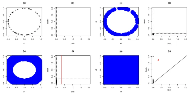
Example 2.1. Point Cloud to Persistence Diagram. We illustrate construction

of the persistence diagram for a point cloud with N = 60 points sampled from the unit circle x2₁+x2₂ = 1:

set.seed(1); PC <- circleUnif(n = 60, r = 1) plot(PC, main = "(a)")

The point cloud is shown in Figure 35(a). We expect to see a total of k0 = 60 values of

˜

α0,k and k1 = 1 value of ˜α1,k. We use the function ripsDiag from the R-TDA package

for constructing the persistence diagram (Fasy et al., 2014). In the R code chunk shown below, PC denotes the input point cloud, maxdimension is the maximum dimension ˜p

of points ˜τp,k˜ to be calculated, and maxscale is the maximum value that the filtration

parameter λ can assume. We set maxdimension to be 1. The default dist is the Euclidean distance. The output pers.diag.1 returns the persistence diagram, as a matrix with three columns which summarize topological features of the point cloud.

(pers.diag.1 <- ripsDiag(X=PC, maxdimension = 1, maxscale = max(dist(PC))) ) $diagram

dimension Birth Death

[1,] 0 0.0000000 1.999999902

(40)

[3,] 0 0.0000000 0.245260715 ...

[60,] 0 0.0000000 0.027923092

[61,] 1 0.3190835 1.737696840

The first row with ˜τ0,1 = (0,2.00) in the output records that there is a 0-th homology

group (connected component) whose birth happens atλ= 0 and whose death happens at about λ= 2.00. The second row with ˜τ0,1 = (0,0.31) records that the second connected

component is born atλ = 0 and is dead atλ= 0.31, etc. We see that all 0-th homology groups have birth time 0, and all N = 60 points start as connected components. These 60 connected components are shown in decreasing order of persistence (slower death). Row 61 with ˜τ1,1 = (0.32,1.74) describes the birth and death of a first homology group

(tunnel) atλ= 0.32 andλ= 1.74 respectively. Figure 35(b) corresponds to the filtration parameter λ= 0 and is obtained using this code:

plot(x=1,y=1,type="n",ylim=c(0,2),xlim=c(0,2),ylab="death",xlab="birth",main="(b)") abline(v = 0, lty = 2)

The dashed vertical line indicates the birth time of connected components; the plot has no points because none of the connected components has died. Figure 35(c) corresponds to the point cloud when λ= 0.1:

(41)

The blue balls Bλ(vi) around each point enlarge and connect with others, resulting in

fewer connected components. The black dots in Figure 35(d) denote the birth-death times of the merged connected components which have died before λ= 0.1:

death.time = sort(pers.diag.1$diagram[pers.diag.1$diagram[, 1]==0, 3])

plot(x = rep(0, sum(death.time<=0.1)), y = death.time[which(death.time<=0.1)], ylim = c(0, 2), xlim = c(0, 2), ylab = "death", xlab = "birth", main = "(d)") abline(v = 0, lty = 2); abline(h = 0.1, lty = 2)

When λ= 0.32 in Figure 35(e), all points connect together and a tunnel emerges, which is the white area surrounded by the blue circle:

plot(PC, pch = 16, cex = 12, col = "blue", main = "(e)")

The birth time of this tunnel is recorded as λ = 0.32, which is shown as the red dashed line in Figure 35(f). Further, there are more black dots in this figure since there are more connected components that have died before λ= 0.32:

plot(x = rep(0, sum(death.time<=0.32)), y = death.time[which(death.time<=0.32)], ylim = c(0, 2), xlim = c(0, 2), ylab = "death", xlab = "birth", main = "(f)") abline(h = pers.diag.1$diagram[pers.diag.1$diagram[, 1]==1, 2], lty = 2) abline(v = 0, lty = 2); abline(v = 0.32, col = "red", lty = 1)

When λ reaches its maximum value of 2 (which is the largest value inDE(vi1,vi2)), the

(42)

-1.0 -0.5 0.0 0.5 1.0 -1.0 -0.5 0.0 0.5 1.0 (a) x1 x2 0.0 0.5 1.0 1.5 2.0 0.0 0.5 1.0 1.5 2.0 (b) birth death -1.0 -0.5 0.0 0.5 1.0 -1.0 -0.5 0.0 0.5 1.0 (c) x1 x2 0.0 0.5 1.0 1.5 2.0 0.0 0.5 1.0 1.5 2.0 (d) birth death -1.0 -0.5 0.0 0.5 1.0 -1.0 -0.5 0.0 0.5 1.0 (e) x1 x2 0.0 0.5 1.0 1.5 2.0 0.0 0.5 1.0 1.5 2.0 (f) birth death -1.0 -0.5 0.0 0.5 1.0 -1.0 -0.5 0.0 0.5 1.0 (g) x1 x2 (h) 0.0 0.5 1.0 1.5 2.0 0.0 0.5 1.0 1.5 2.0 Birth Death

Figure 5: Persistence diagram corresponding to a point cloud. (a) shows the raw point cloud and (h) shows the persistence diagram. (c), (e) and (g) are intermediate steps for the filtration by varyingλ, while (b), (d) and (f) are intermediate steps for constructing the persistence diagram.

shows the birth-death times for all connected components (the dots) and the tunnel (the red triangle):

plot(PC, pch = 16, cex = 40, col = "blue", main = "(g)") plot(pers.diag.1$diagram, main = "(h)")

R-TDAalso supports construction of a persistence diagram given an arbitrary distance matrix as input, as shown in the example below.

Example 2.2. Distance Matrix to Persistence Diagram. The input to ripsDiag

can be a distance matrix computed from the point cloud generated in Example 2.1. Here, we use the defaultdist="euclidean". Other options are"manhattan","maximum", etc.

(43)

dist.PC <- dist(PC)

(pers.diag.2=ripsDiag(X=dist.PC,dist="arbitrary",maxdimension=1,maxscale=max(dist.PC))) $diagram

[1,] 0 0.0000000 1.999999902 [2,] 0 0.0000000 0.306978455 [3,] 0 0.0000000 0.245260715 ... [60,] 0 0.0000000 0.027923092 [61,] 1 0.3190835 1.737696840

2.3.2 Distances Between Persistence Diagrams

Two distance metrics are commonly used to quantify the dissimilarity between two persistence diagrams ˜Ω1 and ˜Ω2 , the Wasserstein distance and the bottleneck distance

(Mileyko et al., 2011). We define these distances and describe their computation using the R-TDA package.

The q-Wasserstein distance between two persistence diagrams is defined by

Wq,p˜( ˜Ω1,Ω˜2) = inf η: ˜Ω1→Ω˜2 X ˜ τp,k˜ ∈Ω˜1 |τ˜p,k˜ −η(˜τp,k˜ )|q∞ 1/q , q= 1,2, . . . , (2.3)

(44)

bottleneck distance of dimension ˜pdefined by W∞,p˜( ˜Ω1,Ω˜2) = inf η: ˜Ω1→Ω˜2 sup ˜ τp,k˜ ∈Ω˜1 |τ˜p,k˜ −η(˜τp,k˜ )|∞. (2.4)

The bottleneck distance is obtained by minimizing the largest distance of any two corre-sponding points of diagrams, over all bijections between ˜Ω1 and ˜Ω2 and is less sensitive

to details in the diagrams.

Example 2.3. Wasserstein and Bottleneck Distances. Let ˜Ω1 be pers.diag.2,

the persistence diagram obtained in Example 2.2. Let ˜Ω2bepers.diag.3, the persistent

diagram we construct from a different point cloud from the same unit circle. We use

R-TDA to compute the Wasserstein distance with q = 1 (denoted by the argument p=1

below):

set.seed(2); PC2 <- circleUnif(n = 60, r = 1)

pers.diag.3 <- ripsDiag(X=PC2, maxdimension = 1,maxscale = max(dist(X))$diagram wasserstein(pers.diag.2, pers.diag.3, p=1, dimension = 0)

1.034579

The function bottleneck enables us to compute the bottleneck distance between the two persistence diagrams. The Wasserstein distance is larger than the bottleneck distance since the former measures more detailed difference between the diagrams.

(45)

0.06954618

It is important to construct persistence diagrams using the same distance functions (Chazal et al., 2018), as we show below. For instance, we can construct a persistence diagram pers.diag.4for the point cloud in Example 2.1 using the Manhattan distance (DM(vi,vj) =

Pd

`=1|vi,`−vj,`|,1≤i, j ≤N) instead of the Euclidean distance.

dist.PC.man <- dist(PC, method = "manhattan"); max.dist=max(dist.PC.man) pers.diag.4=ripsDiag(X=dist.PC.man,dist="arbitrary",maxdimension=1, maxscale=max.dist)$diagram

wasserstein(pers.diag.2, pers.diag.4, p=1, dimension = 0) 2.145083

bottleneck(pers.diag.2, pers.diag.4, dimension = 0) 0.8279462

2.3.3 TDA of Time Series via Point Clouds

Time series do not naturally have point cloud representations, and are transformed to point clouds using Takens’s Embedding Theorem (Takens et al., 1981) before we can do TDA as discussed in Section 2.3.1. This approach has been used in the literature mostly for quantifying periodicity in time series (Perea and Harer, 2015), clustering time series (Seversky et al., 2016), classifying time series (Umeda, 2017), or finding early signals for critical transitions (Gidea, 2017; Gidea and Katz, 2018). Takens’s

(46)

embedding guarantees the preservation of topological properties of a time series but not its geometrical properties.

Takens’s Delay Embedding for Time Series

Let {xt, t = 1,2, . . . , T} denote an observed time series. We use Takens’s embedding

to convert the time series into a point cloud with points vi = (xi, xi+τ, . . . , xi+(d−1)τ)0,

where d specifies the dimension of the points and τ denotes a delay parameter. For example, if d = 2 and τ = 1, then, vi = (xi, xi+1)0, whereas if d = 15 and τ = 2,

vi = (xi, xi+2, . . . , xi+28)0. Both d and τ are unknown and must be determined in

practice.

Choice of τ. Researchers have used different approaches for choosing the delay

param-eter τ. It may be selected as the smallest time lag h where the sample autocorrelation function (ACF) ˆρh becomes insignificant, i.e., smaller in absolute value than the critical

bound √2

T (Khasawneh and Munch, 2016). Truong (2017) also used the ACF, but in

a slightly different way. He chose τ as the smallest lag for which ( ˆρτ −ρˆτ−1)/ρˆτ > 1/e

and ˆρτ < √2_T. Pereira and de Mello (2015) determined τ using the first minimum of

the auto mutual information (the mutual information between the signal and its time delayed version).

Choice of d. Truong (2017) and Khasawneh and Munch (2016) used the false nearest

(47)

integer such that the nearest neighbors of each point in dimension d remain nearest neighbors in dimension d+ 1, and the distances between them also remain about the same. Alternately, an R function false.nearest in the package tseriesChaos which implements an approach due to Hegger et al. (1999) may be used. Some authors (Pereira and de Mello, 2015; Seversky et al., 2016), simply assumedto be 2 or 3, while Perea has suggested the use ofd = 15 on time series after a cubic spline interpolation (see Section 2.3.3).

The choice of d and τ then determine the number of points N in the point cloud. In Example 2.4, we illustrate one approach for constructing a point cloud from pure periodic signals with no noise and then obtaining a persistence diagram. In Example 2.5, we discuss another approach described in Perea et al. (2015) for noisy time series, when the focus is on finding series with the same periodicity.

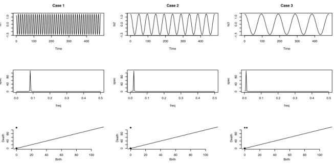
Example 2.4. Pure Signals to Persistence Diagrams. We generate point clouds

from three periodic cosine signals of length T = 480 with periods 12, 48, and 96 respec-tively, and then construct their persistent diagrams. We set d = 2, and use the ACF method discussed above to choose τ. We show R code for the time series ts1:

per1=12;ts1 = cos(1:T*2*pi/per1);d=2;

tau <- which(abs(acf(ts.ex, plot = F)$acf) < 2/sqrt(T))[1]-1

PC=t(purrr::map_dfc(1:(T-(d-1)*tau+1),~ts.ex[seq(from=.x, by=tau, length.out=d)])) diag=ripsDiag(PC, maxdimension=1, maxscale=max(dist(PC)))

(48)

ts.plot(ts.ex);plot(PC,xlab ="x1",ylab="x2",main="PC");plot(diag$diagram)

In Figure 6, the top row shows the signals, the middle row shows the point clouds and the bottom row shows the persistence diagrams. The black dots represent the birth-death of 0-th homology groups and their persistence shows the dispersion of the points in the point cloud. When there are more black dots close to the diagonal, the point cloud is more dispersed. Particularly, the point cloud PC.3 from the time series with period 96 have points close to each other compared with PC.1, so that it has more black dots in the persistence diagram closer to the diagonal.

The red triangles represent the birth-death of first homology groups, indicating circles in the point cloud. The red triangle from the time series with period 96 is further away from the diagonal compared to the series with period 12, and thus has longer persistence in the first homology group. Seeing a circle indicates that the time series is periodic. This is in contrast to the persistence diagram for the same time series based on sublevel set flitration of a function, as discussed in Example 3.2.

Pairwise bottleneck distances between the three persistence diagrams are shown in Table 1, computed using code as shown below:

round(bottleneck(diag1$diagram, diag2$diagram, dimension = 0), digits = 2)

To study the effect ofd, we repeat the computations ford= 3 andd= 15 and also show all pairwise bottleneck distances in the table. While the values of the distances between the diagrams change as d changes, the relative behavior is preserved, independent of d.

(49)

Time ts1 0 100 200 300 400 -1.0 0.0 1.0 Time ts2 0 100 200 300 400 -1.0 0.0 1.0 Time ts3 0 100 200 300 400 -1.0 0.0 1.0 -1.0 -0.5 0.0 0.5 1.0 -1.0 0.0 1.0 PC.1 x1 x2 -1.0 -0.5 0.0 0.5 1.0 -1.0 0.0 1.0 PC.2 x1 x2 -1.0 -0.5 0.0 0.5 1.0 -1.0 0.0 1.0 PC.3 x1 x2 0.0 0.5 1.0 1.5 2.0 0.0 1.0 2.0 Birth Death 0.0 0.5 1.0 1.5 2.0 0.0 1.0 2.0 Birth Death 0.0 0.5 1.0 1.5 2.0 0.0 1.0 2.0 Birth Death

Figure 6: Pure Periodic Signals to Persistence Diagrams.

Specifically, the bottleneck distances between ˜Ω1 and ˜Ω2 and between ˜Ω1 and ˜Ω3 are

larger than the distance between ˜Ω2 and ˜Ω3 in the 0-th and first homology groups.

Table 1: Pairwise Bottleneck Distances Between Persistence Diagrams for Different d.

d= 2 d= 3 d= 15

(1,2) (1,3) (2,3) (1,2) (1,3) (2,3) (1,2) (1,3) (2,3) 0th 0.26 0.26 0.07 0.36 0.36 0.09 0.73 0.73 0.18 1th 0.39 0.45 0.06 0.53 0.63 0.09 1.09 1.28 0.19

Point Cloud Construction using SW1PerS

The SW1PerS (Sliding Windows and 1-Persistence Scoring) method is an alternate, more comprehensive approach proposed by Perea et al. (2015) to detect periodicity from noisy time courses whose underlying signals may have different shapes. The approach addresses the following items.

(50)

the user. The first type smooths the raw time series by a moving average in order to make it easier to detect the signal. The second type is a moving average on the point cloud. As an alternative to moving averaging, Pereira and de Mello (2015) used the Empirical Mode Decomposition (EMD) (Huang et al., 1998) on the raw time series.

Spline Interpolation. The spline interpolation allows handling unevenly spaced time

series, or time series with low temporal resolution.

Point Cloud Standardization. Standardization helps with signal dampening and to

make the procedure amplitude blind.

The pipeline for this approach is described in the following steps.

Step 0. Optionally (Perea and Harer, 2015), denoise the observed time series {xt, t =

1,2, . . . , T}using a simple moving average whose window size is no higher than one

third of the selected dimensiond. They recommended an embedding dimension of

d= 15 and N = 201 as the size of the point cloud; then T1 =N +d= 216.

Step 1. For selected values of d and τ (see below), create a point cloud from the

(pos-sibly denoised) time series using Steps 1.1 and 1.2.

Step 1.1. Recover a continuous function g : [0,2π]→ R by fitting a cubic spline to the denoised time series {xt, t= 1,2, . . . , T}.

Step 1.2. Using valuesg(t1), g(t2), . . . , g(tT1) from the continuous spline fitg(.) at evenly

(51)

point cloud withN =T1−dpointsv (0)

t = (g(t), g(t+τ), . . . , g(t+(d−1)τ))0 ∈

Rd_{, t}_{= 0}_{, τ, . . . ,}₂_π₋₍_d₋₁₎_τ _{and so}_τ ₌ 2π

N+d−1.

Step 2. Pointwise Point cloud standardization:

vt= v_t(0)−¯v_t(0)1 ||v_t(0)−¯v_t(0)1||; v¯ (0) t = d X i=1 v_t,i(0)/d, ||v(0)_t −¯v_t(0)1||= v u u t d X i=1 (v(0)_t,i −v¯(0)_t )2_, (2.5)

where v_t(0) = (v_t,(0)₁, v_t,(0)₂, . . . , v_t,d(0))0 and 1is the d-dimensional vector of 1’s.

Step 3. Construct the persistence diagram from the point cloud as shown in Section

2.3.1.

This method is powerful for detecting periodicity in time series. To develop a score for quantifying the periodicity, Perea et al. (2015) first found the longest persistence of the birth-death of the first homology groups (λ1,kM,1, λ1,kM,2), wherekM = arg maxk(λ1,k,2− λ1,k,1) is chosen to indicate maximum persistence, and used it to compute

S = 1− λ 2 1,kM,2−λ 2 1,kM,1 3 . Since 0 ≤ λ1,kM,1 ≤ λ1,kM,2 ≤ √

3, for periodic (nonperiodic) time series, the score is close to zero (one). The R code for implementing Step 1-Step 3 for Case 1 is shown below (the code for other cases is similar):

(52)

x.ts = ts1; d=15; N=201; T1 = 216;

x.ts <- pracma::movavg(x.ts, 5, type = "s") #step 0

sp.ts <- stats::spline(1:T*2*pi/T, x.ts, n=T1)$y #step 1.1 PC <- plyr::ldply(map(1:N, ~sp.ts[.x:(.x+d-1)]))#step 1.2

X.PC=t(apply(PC,1,FUN=function(x){(x-mean(x))/sqrt(sum((x-mean(x))^2))})) #step2 diag <- ripsDiag(X=x.PC, maxdimension = 1, maxscale = sqrt(3))#step 3

The main contributions of Perea et al. (2015) are the use of extensive simulation studies to show that topological features of time series are largely the same under various non-sinusoidal shapes as well as under differences in amplitude, phase, mean, frequency, or trend. The results may be affected by a differences in noise variances, as well as by the shapes of the noise and signal distributions.

Example 2.5. Using SW1PerS for Periodicity Quantification. We generate

white noise t with variance σ2 = 0.64, and then generate periodic time series signals

each of length T (= 480), denoted by ts1, ts2, ts3, ts4, and shown in the top row of Figure 7.

• Case 1: xt = cos(2πt/12) +t,

• Case 2: xt = 0.05t+ 10(cos(2π(t−ϕ)/48) +t), • Case 3: xt = 10(cos(2πt/12) +t) exp (−0.01t), • Case 4: xt =t

(53)

The series ts2 differs from ts1 in frequency, phase, and linear trend, whereas ts3

only differs from ts1 in shape and amplitude; ts4 is the white noise series. Figure 7 shows that the method in Perea et al. (2015) is insensitive to different periodicities. The top row shows the simulated time series under the four cases. The middle row presents a two dimensional view of the point clouds constructed with d = 15 and τ = 1, via the first two principal components. The bottom row shows the persistence diagrams, along with the periodicity score S. For periodic (nonperiodic) time series, the score is close to zero (one), so that the scores for Case 1 to Case 3 are close to 0, while Case 4 has a score close to 1.

2.4 Persistent Homology Based on Functions

We first give a basic review of TDA based on functions, followed by the use of frequency domain representations of time series as starting points for TDA.

2.4.1 Function to Persistence Diagram - A Basic Review

When data is in the form of a continuous function f : Rd _{→ R}_{, or can be converted}

to such a function, TDA using sublevel set filtration is carried out by discretizing the function into grids and then implementing computational homology on the dis-cretized function. Suppose the components of the function arez= (`1δ, `2δ, . . . , `dδ), for

(54)

Case 1 Time 0 300 -2 0 2 Case 2 Time 0 300 -20 10 40 Case 3 Time 0 300 -15 0 15 Case 4 Time 0 300 -1.5 0.5 -1.0 0.5 -1.0 0.0 1.0 PC1 PC2 -1.0 0.5 -1.0 0.0 1.0 PC1 PC2 -1.0 0.5 -1.0 0.0 1.0 PC1 PC2 -1.0 0.5 -1.0 0.0 1.0 PC1 PC2 S=0.219 0.0 1.0 0.0 1.0 Birth Death S=0.157 0.0 1.0 0.0 1.0 Birth Death S=0.191 0.0 1.0 0.0 1.0 Birth Death S=0.85 0.0 1.0 0.0 1.0 Birth Death

(55)

defined as

Lλ(f) ={z:f(z)≤λ,z∈ Rd}, (2.6)

where 0≤ λ≤ maxzf(z). Define a simplex as a set of components in Lλ(f) which are

“neighbors”, i.e., z1,z2 ∈Lλ(f), and |z1,j−z2,j| ≤δ, j= 1,2, . . . , d.

Recall from Section 2.3.1 that a simplex with (˜p + 1) components is called a ˜p -simplex. Since only adjacent points on the grid can be neighbors, the function f(z) can admit at most a d-simplex, so that ˜p ≤ d−1 (Edelsbrunner and Harer, 2010). When

d = 1, there are only connected components, whose births and deaths are given by ˜

τ0,k = (λ0,k,1, λ0,k,2), k= 1,2, . . . , k0. The computations in the steps that are summarized

below are done using the R function gridDiag(Fasy et al., 2014).

Step 1. Assume a filtration parameter starting at λ = minzf(z) and let Lλ(f) = {z :

f(z) = minzf(z)}.

Step 2. Construct topological features for increasing values ofλ. For eachλ, simplicial

complexes can be constructed from the sublevel set Lλ(f), and ˜αp,k˜ can be

com-puted using computation homology, where 0 ≤ p˜≤ d−1. If an elder topology ˜

αp,k˜ 1 and a younger topology ˜αp,k˜ 2 merge into a single ˜αp,k˜ at some λ value, then

˜

αp,k˜ 1 becomes ˜αp,k˜ and ˜αp,k˜ 2 dies at λ, using the Elder Rule (Edelsbrunner and

Harer, 2010).

Step 3. The persistence diagram is the output of the set of points representing

(56)

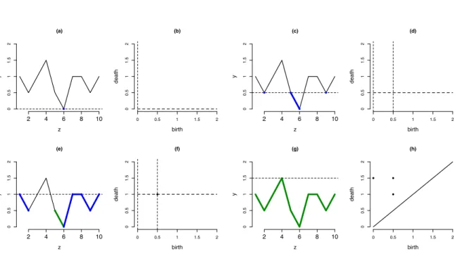
Example 3.1. Discretized Function to Persistence Diagram. We present an example of using TDA on a one-dimensional discretized real function generated using the code chunk below, where funval contains values of the function taken over a grid:

funval = c(1, 0.5, 1, 1.5, 0.5, 0, 1, 1, 0.5, 1)

(pers.diag.4 <- gridDiag(FUNvalues = funval, sublevel = TRUE) ) $diagram

[1,] 0 0.0 1.5

[2,] 0 0.5 1.5

[3,] 0 0.5 1.0

The persistence diagram contains three connected components born at λ = 0 and λ = 0.5, corresponding to the function having three local minima at these two distinct λ

values. In Figure 23(a), a connected component emerges when λ = 0 and is marked as a blue dot (it is the earliest/oldest connected component).

plot(funval, x=1:10, type = "l",yaxt=’n’,ylim = c(0,2), cex.axis=1.4, xlab = "z", ylab= "y", cex.lab= 1.3, cex=1.2, lwd=1.5, lty=1, pch=1, bty=’n’, main="(a)") points(x=6, y=0, pch=16, col="blue", type = "p")

ticks<-c(0, 0.5, 1, 1.5, 2); axis(2,at=ticks,labels=ticks) abline(a=0, b=0, lty=2, lwd=1,pch=1)

(57)

the horizontal dashed line tracks the current filtration parameter λ. There is no point on the birth/death plot yet, as no connected components have died at λ= 0.

plot(rep(0,11),x=0:10/5,type = "l",cex.axis=1.4,xaxt=’n’,xlab= "birth",yaxt=’n’, ylim=c(0,2),ylab="death",cex.lab=1.3,cex=1.2,lwd=1.5,lty=2,pch=1,bty=’n’,main="(b)") axis(1,at=ticks,labels=ticks); axis(2,at=ticks,labels=ticks); abline(v=0, lty=2)

Figure 23(c) corresponds to λ = 0.5. There are two more connected components indicated by the blue dots at (2,0.5) and (9,0.5). The blue dot (6,0) in the middle with a blue line connecting it to the dot (5,0.5) indicates that the oldest connected component enlarges.

plot(funval, x=1:10, type = "l",yaxt=’n’,ylim = c(0,2),cex.axis=1.4,xlab = "z", ylab = "y",cex.lab= 1.3, cex=1.2,lwd=1.5, lty=1, pch=1, bty=’n’, main = "(c)") axis(2,at=ticks,labels=ticks); abline(a=0.5, b=0, lty=2, lwd=1,pch=1)

points(x=6, y=0, pch=16, col="green4", type = "p",xlab = "z", ylab= "y")

points(x=c(2,5,9), y=rep(0.5,3), pch=16, col="blue", type = "p",xlab="z",ylab="y") segments(x0=6, y0=0, x1=5, y1=0.5, lty = 1, pch=1, lwd=2.5, col = "blue")

Figure 23(d) has one more vertical dashed line, which gives the birth time for the other two new connected components. There is no connected component dead yet, and so no points are shown on the second plot either. The code chunks for plotting these are similar and are not shown due to space limitations. Whenλ= 1, in Figure 23(e), all components enlarge and one newer component is killed by the elder one because they

(58)

2 4 6 8 10 (a) z y 0 0.5 1 1.5 2 (b) birth death 0 0.5 1 1.5 2 0 0.5 1 1.5 2 2 4 6 8 10 (c) z y 0 0.5 1 1.5 2 (d) birth death 0 0.5 1 1.5 2 0 0.5 1 1.5 2 2 4 6 8 10 (e) z y 0 0.5 1 1.5 2 (f) birth death 0 0.5 1 1.5 2 0 0.5 1 1.5 2 2 4 6 8 10 (g) z y 0 0.5 1 1.5 2 (h) birth death 0 0.5 1 1.5 2 0 0.5 1 1.5 2

Figure 8: Construction of a persistence diagram corresponding to a one-dimensional continuous real function. (a) is the function and (h) is the persistence diagram. (c), (e) and (g) show the sublevel set filtration procedure, while (b), (d) and (f) are the intermediate steps for constructing the persistence diagram.

are merged. There is a black dot at (0.5,1) in Figure 23(f), which indicates the newer connected component that is born at λ = 0.5 and is dead at λ = 1. When λ = 1.5 reaching the maximum of the function in Figure 23(g), the last component is killed. The black dot at the location (0,1.5) in Figure 23(h) is for the last component. The other black dots corresponding to (0.5,1.5) and (0.5,1) show the birth and death of other connected components.

Example 3.2. Morse Function to Persistence Diagram. An alternate technique

for persistent homology which is robust to noisy point cloud data uses the R function

gridDiag (Chazal et al., 2018). As mentioned in the introduction, a point cloud is

(59)

gridDiag enables us to construct a Morse function such as the distance-to-measure (DTM) function from the point cloud using the sublevel set filtration. Suppose the point cloud is {xi ∈ Rd, i = 1,2, . . . , N}. Represent the DTM function from Rd → R

as f(DT M)(x) = s X xi∈Nk(x) ||xi−x||2/k,

where k= [mN] (m is the parameter m0) and Nk(x) is the set containing thek nearest

neighbors of x in the point cloud.

A higher value of f(DT M)(x) means that x is further away from most of the points. DTM is also robust to outliers (Chazal et al., 2018). We illustrate using the same point cloud data from Example 2.1:

m0=0.05; by <- 0.065; Xlim <- range(PC[,1]); Ylim <- range(PC[,2])

(pers.diag.5 = gridDiag(X=PC, FUN=dtm, lim=cbind(Xlim, Ylim), by=by, m0=m0) ) $diagram

[1,] 0 0.02414385 0.96912324 [2,] 0 0.02623549 0.15885911 [3,] 0 0.03489488 0.15662338 ... [20,] 0 0.14527336 0.15092905 [21,] 1 0.20234735 0.96912324