Constructing a No-Reference H.264/AVC
Bitstream-based Video Quality Metric using Genetic
Programming-based Symbolic Regression
Nicolas Staelens,
Associate Member, IEEE,
Dirk Deschrijver,
Member, IEEE,
Ekaterina Vladislavleva,
Member, IEEE,
Brecht Vermeulen, Tom Dhaene,
Senior Member, IEEE,
and Piet Demeester,
Fellow, IEEE
Abstract—In order to ensure optimal Quality of Experience towards the end-users during video streaming, automatic video quality assessment becomes an important field-of-interest to video service providers. Objective video quality metrics try to estimate perceived quality with a high accuracy and in an automated manner. In traditional approaches, these metrics model the complex properties of the Human Visual System. More recently, however, it has been shown that Machine Learning approaches can also yield competitive results. In this article, we present a novel No-Reference bitstream-based objective video quality metric that is constructed by Genetic Programming-based Symbolic Regression. A key benefit of this approach is that it calculates reliable white-box models that allow us to determine the importance of the parameters. Additionally, these models can provide human insight into the underlying principles of subjective video quality assessment. Numerical results show that perceived quality can be modeled with a high accuracy using only parameters extracted from the received video bitstream.
Index Terms—Quality of Experience (QoE), Objective video quality metric, No-Reference, H.264/AVC, High Definition.
I. INTRODUCTION
D
URING real-time transmission of digital video over best-effort Internet Protocol (IP)-based networks, packet losses can severely degrade the overall Quality of Experience (QoE) of the end-users [1]. This, in turn, influences willingness to pay and customer satisfaction [2], [3]. Furthermore, QoE is considered a key factor for the success or failure of new broadband video services [4]. Therefore, services providers strive towards maximizing and maintaining adequate QoE at all times. In the case of video streaming, this requires contin-uous monitoring and measuring of perceived video quality in order to get an indication of end-users’ QoE.Subjective video quality assessment is commonly used to measure the influence of visual degradations on perceived quality of video sequences [5]. During subjective quality assessment, real human observers evaluate the visual quality of a number of short video sequences by, for example, providing a score between 1 (bad) and 5 (excellent) after or while watching each video sequence. Afterwards, the Mean Opinion Score (MOS) is calculated per video sequence as the average quality N. Staelens, D. Deschrijver, B. Vermeulen, T. Dhaene and P. Demeester are with Ghent University - iMinds, Department of Information Technology, Ghent, Belgium (e-mail:{nicolas.staelens, dirk.deschrijver, brecht.vermeulen, tom.dhaene, piet.demeester}@intec.ugent.be).
E. Vladislavleva is with Evolved Analytics Europe BVBA, Wijnegem, Belgium (e-mail: [email protected]).
rating provided by the different observers. Several assessment methodologies have already been standardized by the Interna-tional Telecommunications Union (ITU) in ITU-T Recommen-dation P.910 [6] and ITU-R RecommenRecommen-dation BT.500-12 [7], and describe in detail how subjective video quality experi-ments should be set up and conducted. However, subjective experiments are time-consuming, expensive and need to be conducted in controlled environments. Furthermore, it is clear that subjective quality assessment cannot be used in the case of real-time quality monitoring and measuring.
Over the past years, a lot of research has been conducted towards the construction of objective video quality metrics. As stated in [8], “The goal of objective image and video quality assessment research is to design quality metrics that can predict perceived image and video quality automatically.”. This rather broad definition can also be refined by stating that this prediction should bereliable and correlate well with scores of subjective quality assessment (= MOS scores).
In this article, the use of a robust Machine Learning (ML) technique, called Symbolic Regression, is proposed to derive a new No-Reference bitstream-based objective video quality metric for estimating perceived quality of High Definition (HD) H.264/AVC encoded videos. The new approach has two distinctive features that make it particularly attractive for the analysis of perceived video quality : a) it allows us to perform an automated selection of the most important variables, and b) it provides predictive models that are interpretive and provide insight in the relation between encoder settings, loss location, and video content characteristics and the perceived quality.
The remainder of this article is outlined as follows. Section II gives an overview of the state-of-the-art and describes how ML algorithms can be used to derive different types of objective video quality metrics. In Section III, the mod-eling principles of the genetic-programming based symbolic regression approach are outlined, and a detailed description of the algorithmic aspects is provided. In order to validate the effectiveness of the proposed method, an extensive subjective experiment was conducted. The procedure that is followed to collect the subjective quality ratings from human observers is discussed in Section IV. Then, Section V presents the main results and describes how the new modeling approach can be applied to derive a new No-reference bitstream-based metric for video quality assessment. First, the different parameters that are extracted from the received encoded video bitstream
are listed and the symbolic regression approach is used to determine the most important parameters. Next, this subset of parameters is selected in the modeling process to compute a final model that predicts the perceived video quality in a reliable way. An interpretation of the model and a comparison with alternative machine learning techniques is also provided. Numerical results confirm that the perceived quality can be predicted accurately using only parameters extracted from the received video bitstream. Section VI concludes the article.
II. MACHINELEARNING-BASEDMETRICS
A. Objective Video Quality Metrics
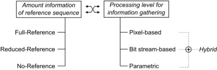
In general, objective video quality metrics can be catego-rized into three main classes, based on the availability of the original video sequences as depicted in Figure 1.
Full-Full-Reference Reduced-Reference No-Reference Pixel-based Bit stream-based Parametric Processing level for information gathering Amount information
of reference sequence
+ Hybrid
Fig. 1. Different categories of video quality metrics based on the amount of information which is used from the reference sequence or based on the processing level for extracting information in order to model perceived quality.
Reference (FR) quality metrics [9] require access to the com-plete original video stream. Research has already shown that FR metrics can predict perceived quality with high accuracy. However, due to their dependency on the original video, FR metrics cannot be used for real-time video quality evalua-tion. Reduced-Reference (RR) metrics, recently standardized in [10], perform quality prediction by comparing features ex-tracted from the original and received video sequence. In order to transmit these features from the points they are extracted to the point where the quality evaluation is performed, an ancillary error-free channel is needed. Both FR and RR metrics usually predict quality based on a frame-by-frame evaluation. As such, the received video stream requires proper alignment with the original sequence. From a real-time monitoring point of view,No-Reference(NR) video quality metrics are the most interesting ones as they neither need access to the original sequence nor rely on feature extraction [11].
Another criterion to categorize these metrics is the type of information or processing level where the information from the video sequences is extracted. As such,pixel-basedmetrics require access to the decoded video stream whereas bitstream-based metrics only perform a parsing of the encoded data. A last category of video quality metrics are the parametric
metrics, which only use high level information accessible through the packet headers in the case of video streaming. Quality metrics combining information from the network-, pixel- and/or bitstream-level are also called hybrid metrics. For real-time video quality evaluation, metrics which do not require a complete decoding of the received video stream are of particular interest. The interested reader is referred to [12]
for more details on the classification of objective video quality metrics and a performance comparison.
The performance of FR and RR video quality metrics has already widely been investigated by the Video Quality Experts Group (VQEG) through several projects [13], [14], [15]. The results of this study resulted in the standardization of a number of objective video quality metrics. However, research is still ongoing towards the construction of NR metrics.
B. Overview of State-of-the-art
Machine learning techniques such as Neural Networks (NN), Support Vector Machines (SVM), Support Vector Re-gression (SVR) and decision trees have already successfully been applied for constructing objective video quality metrics. In general, these metrics either use regression or classification for estimating perceived quality. Regression is commonly used for estimating MOS whereas classification is typically used for predicting error visibility by means of a binary decision.
In [16] and [17], Mohamedet al.used NNs for constructing an objective video quality metric capable of continuous qual-ity monitoring and measuring. The stream bitrate, sequence frame rate, network loss rate and burst size, and the ratio of encoded intra to inter macroblocks are used as inputs to the NN. However, only a single low resolution (352x288 pixels1) video sequence was used for training and validating
the model. Consequently, the influence of video content is not considered in the proposed model. Nevertheless, results indicated that quality can be estimated with a high accuracy without the need for modeling the Human Visual System (HVS). A similar approach is followed in [18], where an NN is used to estimate perceived quality of H.264/AVC encoded CIF resolution sequences. However, the authors do not consider the influence of network impairments on the perception of quality. NNs have further also been used in [19], [20] and [21] for modeling video quality.
Recently, SVMs have been used to predict video quality. In [22], different NR and RR parameters are extracted from the decoded video stream and used to build an SVM. The performance of the model is evaluated based on an existing FR objective video quality metrics, VQM [23]. Compared to their previous work [24], the authors found that video quality can be predicted with a higher accuracy using SVMs. Also Nar-waria et al.[25], [26], [27] model visual quality using SVR. More specifically, ML is used for modeling the interaction effect between spatial and temporal quality factors affecting perveived video and image quality. In [27], they evaluate the performance of SVR on a number of video databases against eight different existing visual quality predictors, and the results show a significant improvement in prediction accuracy.
Rather than estimating the perceived quality, Argyropoulos
et al. use SVMs in [28] and [29] to build a classifier for estimating the probability that an impairment in the video stream will result in a visible impairments for the end-user.
In [30] and [31], packet loss visibility is estimated using decision trees. In this case, a binary classification is performed labeling an impairment in the video bitstream as visible or
invisible to the average end-user. A decision tree is also used by Menkovski et al. [32] to determine whether the QoE of a video service is acceptable or not acceptable. As a decision tree is a white box model, the internal structure of the classification process is completely visible and can thus be used to gain better insights in the modeling process. This is not the case for SVMs and NNs, which are black-box models. In our previous work [33], we investigated and modeled impairment visibility in HD H.264/AVC encoded video se-quences using decision trees. Our results showed that it is possible to reliably predict impairment visibility using only a limited number of parameters extracted from the received video bitstream. As a decision tree was used, a binary classi-fication is made. The work presented in this article further elaborates on the data obtained during our previous work. However, instead of determining impairment visibility we are now interested in estimating how end-users would rate the visual quality of the video sequences. As such, our goal is to construct a video quality metric which predicts perceived quality and correlates well with the MOS obtained during subjective quality assessment.
III. GP-BASEDSYMBOLICREGRESSION
In this section, a novel ML technique (Genetic Programming (GP)-based symbolic regression method [34]) is proposed to model the perceived quality, as an alternative to modeling the different complex properties of the HVS. As the name suggests, this method is applied to model the MOS score by means of a regression approach (not classification). A key advantage of this method is that the resulting metrics are essentially white-box models that comprise only the variables that are truly influential. Moreover, the metric can provide human insight into the underlying principles of subjective video quality assessment.
A. Goal statement and notation
GP-based symbolic regression offers the unique capability to compute non-linear white-box models that predict the MOS quality rating q of a video fragment in terms of several input variables ~v = {vn}Nn=1. These variables ~v identify the characteristics of the sequence and quality degradation factors, and comprise only those parameters that can be extracted from the received video bitstream without the need for complete decoding. Given a limited set ofM video sequences, a sparse set of data samples S is obtained, which can be represented as a set of tuplesS={(~vm, qm)}Mm=1. Symbolic regression is then used to compute a set of modelsf that predict the MOS quality scores qin terms of the parameters~v [35]:
f:RN →R, f(~vm)≈qm (1) A set of models is calculated, because this allows us to determine the importance of variables in a reliable way. As suggested by El Khattabi et al. [21], one should only retain the relevant input variables, in order to reduce the computional cost and to limit the model complexity. The importance of carefully selecting the input variables for subjective video
quality assessment was also highlighted in [35]. After discard-ing the redundant variables, a new set of models is computed using only the most important variables and the best model is returned as the final solution. Note that for the actual im-plementation, we made use of the DataModeler package [36] for Mathematica, because it offers the integrated functionality for automatic variable selection and dimensionality analysis, variable contribution analysis and set-based predictions.
B. Outline of Evolutionary Algorithm
This section explains some algorithmic details on how the set of models can be computed in a reliable way. GP-based symbolic regression is a biologically inspired method that mimics the process of Darwin’s evolution theory and the mechanisms of genetic variation and natural selection [37]. It is based on the concept of genetic programming, and computes a set of tree-based regression models that give a good approximation of the sparse subjective video quality data S. The evolutionary algorithm consists of the following steps: 1) Model initialization : In the first generation step
(t= 1), an initial population ofK randomly generated parse trees Pt = {f
k(~v)}Kk=1 (also called models or individuals) with a maximal arity of 4 is formed. Each parse tree fk(~v) represents a potential solution to the approximation problem, and is composed of multiple nodes that comprise primitive functions and terminals. The primitive functions are represented by the standard arithmetic operators(+,−,∗, /, inv, pow, sqrt,ln,exp), whereas the terminals consist of the input variables~vand real constants drawn from the interval [−5,5]. All the input variables~v are scaled into the range {0...2}. 2) Model evaluation: In order to measure the fitness of a
particular individual, an operatorZ is defined that maps each model onto the space of two design objectives.
Z :fk(~v)∈Pt→(z1(fk(~v)), z2(fk(~v)))∈Θ (2) • Objective 1 aims to minimize the prediction error
z1(fk(~v)) = 1−R2(q, fk(~v)) (3) whereR represents the correlation coefficient
R(q, fk(~v)) =
cov(q·fk(~v))
std(q)·std(fk(~v))
(4) • Objective 2 aims to minimize the expressional model complexity z2(fk(~v)), which is defined as the sum of the number of nodes in all subtrees of a given tree. This objective penalizes complexity and avoids the excessive growth of models over time. Both criteria are often conflicting, so the goal is to obtain models that make a good trade-off and perform well on both objectives. This idea is motivated by Occam’s razor, which states that simpler models are preferable to more complex ones if they explain the data sufficiently well. 3) Model archiving and elitism : Next to the population
Pt, the algorithm also maintains a fixed-size archive
Atthat contains the best performing models discovered so far. This archive serves as an elistism strategy to
ensure that the fittest models of the population are carried forward from one generation to the next. In each generation stept, the archiveAtis updated by selecting the least-dominated models from the joint setAt−1∪Pt, where initiallyA0=φ. Note that a modelf
1(~v)is said to dominate a modelf2(~v)in the objective space Θif
f1(~v) is no worse than f2(~v)in all the objectives, and strictly better in at least one of the objectives
∀i= 1,2 :zi(f1(v~))≤zi(f2(~v)) (5) ∃j∈ {1,2}:zj(f1(~v))< zj(f2(~v)) (6) (Models that are not outperformed by any other model in terms of both objectives are “pareto-optimal” models) 4) Model evolution : In each step t of the algorithm, a set of individuals is chosen by means of a Pareto tournament selection operator. These individuals are exposed to genetic operators (such as crossovers and mutations), in order to create the population Pt+1 of the next generation step. The crossover operator selects two parent individuals and combines them to create new offspring by swapping sub-trees, whereas the mutation operator makes a random alteration to nodes of a sub-tree. At each generation, archive members (At) are merged with the newly created population (Pt), and variation operators are applied to the aggregated set of models. Selection of individuals for crossovers and mutations happens by means of Pareto tournaments. This archive-based selection preserves genotypic diversity of the individuals. New individuals are generated using a sub-tree crossover with rate 0.9, and sub-tree mutation with rate 0.1. Every 10 generations, the population gets re-initialized to provide diversity and avoid inbreeding. This evolutionary process is repeated over many generation steps (t= 1, ..., T), in order to create models with increasing fitness, based on the survival-of-the-fittest principle. The set-tings of the algorithm are illustrated in Table I. After a certain stopping criterion is met (e.g. a time budget), the algorithm is terminated. All the archivesAtin each run are aggregated into a compound archive A, and the non-dominated individuals in
A are used to form a super Pareto front of models. This set of models is then returned as the final result.
TABLE I
PARETOGPEXPERIMENTAL SETTINGS
Setting Values # replicates 5 # generations 310 population size 1000 archive size 100 crossover rate 0.9
subtree mutation rate 0.1 population tournament 5
IV. SUBJECTIVEVIDEOQUALITYEXPERIMENT In order to validate the method, a subjective video quality experiment was conducted. During the experiment, a number
of test subjects had to evaluate the visual quality of a number of impaired video sequences. This section provides details of the experiment, as well as the selection, encoding and impairing of the different video sequences that were used.
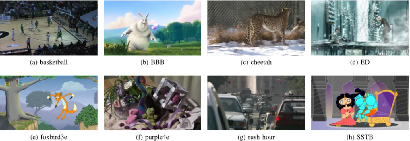
A. Source video sequence selection
As a base for the subjective experiment, eight freely avail-able source video sequences were selected. These sequences were obtained from open source movies, the Consumer Digital Video Library (CDVL) [38] and the Technical University of Munich (TUM). All sequences were in full 1080p HD resolution (1920x1080), with a frame rate for 25 frames per second and a duration of exactly 10 seconds. An overview of the different source sequences is shown in Figure 2, and a short description of their characteristics is provided in Table II. Marked sequences (∗) were taken from an open source movie. It is generally known that certain video characteristics, i.e. the
TABLE II
CHARACTERISTICS OF THE EIGHT SELECTED TEST SEQUENCES. Sequence Source Description
basketball CDVL Basketball game with score. Camera pans
and zooms to follow the action.
BBB* Big Buck
Bunny
Computer-Generated Imagery. Close-up of a big rabbit. Slight camera pan while follow-ing a butterfly in front to the rabbit.
cheetah CDVL Cheetah walking in front of a chainlink
fence. Camera pans to follow the cheetah.
ED* Elephants
Dream
Computer-Generated Imagery. Fixed camera focusing on two characters. Motion in the background.
foxbird3e CDVL Cartoon. Fox running towards a tree and
falling in a hole. Fast camera pan with zoom.
purple4e CDVL Spinning purple collage of objects. Many
small objects moving in a circular pattern.
rush hour TUM Rush hour in Munich city. Many cars
mov-ing slowly, high depth of focus. Fixed cam-era.
SSTB* Sita Sings
the Blues
Cartoon. Close-up of two characters talking. Slight camera zoom in.
amount of motion and the amount of spatial details, influence the perceptibility of visual degradations [39], [40]. Therefore, it was ensured during the subjective video quality assessment that these video sequences have different amounts of motion and textures [6]. For quantifying the amount of motion and spatial details in a video sequence, two perceptual metrics are defined in ITU-T Recommendation P.910: theSpatial percep-tual Information (SI)and theTemporal perceptual Information (TI). These measurements are calculated frame-by-frame and the maximum value is taken as overall SI and TI value for a particular video sequence. However, Ostaszewska et al. [41] showed that the overall SI and TI of a video sequence can be better approximated by taking the upper quartile value instead of the maximum value as this eliminates the influence of peak values (caused by, for example, scene cuts). Hence, the SI and TI value of a video sequence were calculated as follows :
Q3.SI = Upperquartiletime{stdevspace[Sobel(Fn)]}. (7)
Q3.T I= Upperquartiletime{stdevspace[Mn(i, j)]}, (8) whereMn(i, j) =Fn(i, j)−Fn−1(i, j).
(a) basketball (b) BBB (c) cheetah (d) ED
(e) foxbird3e (f) purple4e (g) rush hour (h) SSTB
Fig. 2. Overview of the eight selected source video sequences, taken from open source movies, CDVL and TUM.
Figure 3 visualizes the calculated Q3.SI andQ3.TI values for each of the selected sequences.
basketball BBB cheetah foxbird 3e purple4e rush hour ED SSTB 0 5 10 15 20 25 30 35 0 10 20 30 40 50 60 70 80 90 Q3 .TI Q3.SI
Fig. 3. Calculated Q3.SI and Q3.TI values for each sequence [41].
B. Encoding and impairment generation
The article is focused on the estimation of perceived quality for HD H.264/AVC encoded video sequences. In order to use realistic encoder settings, the settings used for HD content available from online video services and websites were an-alyzed. Furthermore, the default settings recommended by a number of commercially available H.264/AVC encoders were investigated. Based on this analysis, x264 was used with the following settings for encoding the video sequences:
• Number of slices: 1, 4 and 8 • Number of B-pictures: 0, 1 and 2
• GOP size [42]: 15 (0 or 1 B-picture) or 16 (2 B-pictures) • Closed GOP structure
• Bit rate: 15 Mbps
This results in a total number of nine different encoder con-figurations. Each encoded video sequence was also carefully visually inspected to ensure no encoding artifacts were present. The open source streamer Sirannon [43] was used to impair the encoded video sequences. First, the raw H.264/AVC Annex B bitstream was packetized into RTP packets according to RFC3984. Then, slice losses were simulated by dropping all
RTP packets carrying data from that particular slice2. Finally, the stream was unpacketized and the resulting impaired bit-stream was saved to a new file. This process is illustrated in Figure 4. It is also possible to use different configurations for
avc-reader nalu-drop classifier avc-packetizer avc-unpacketizer writer
Fig. 4. RTP packets, which carry data from particular slices, are dropped using thenalu-drop classifiercomponent. After unpacketizing, the resulting impaired sequence is saved to a new file.
dropping slices, by considering on the following parameters: • Number of B-pictures (0, 1, 2)
• Type of first lost slice (I, P, B)
• Location within the GOP of the loss (begin, middle, end) • Number of consecutive slice drops (1, 2, 4)
• Location within the picture of the loss (top, middle, bottom)
• Number of consecutive entire picture drops (0, 1) An experimental design was used to select a subset of 48 representative impairment scenarios which are applied to the eight selected sequences. This resulted in a total amount of
M = 384 impaired video sequences. Note that no visual impairments were injected in the first and last two seconds of video playback. The interested reader is referred to [33] for more details on the experimental design.
For decoding the impaired sequences, a modified version of the JM Reference Software version 16.1 was used, which implements frame copy as concealment strategy [44], [45].
C. Subjective quality assessment methodology
The different encoded and impaired video sequences were presented to human subjects using a Single Stimulus (SS) Ab-2Entire slices should be dropped in order for the bitstream to remain compliant with Annex B as specified in the H.264/AVC video coding standard.
solute Category Rating (ACR) subjective assessment method-ology, as specified in ITU-T Rec. P.910 [6]. The SS methodol-ogy implies that all sequences are presented one-after-another, as depicted in Figure 5. Immediately after watching each sequence, subjects are required to evaluate the quality of that particular sequence using a 5-grade ACR scale with adjectives. Before the start of the experiment, all subjects received specific
~10s ~10s ~10s voting voting Ai Silence/ Bj Ck Grey Silence/ Grey ≤10s ≤10s
Sequence B under test condition j Sequence A under test condition i Sequence C under test condition k Ai
Bj Ck
Fig. 5. Typical trail structure of a SS subjective quality experiment defines the order how sequences are displayed and rated by the subjects.
instructions on how to evaluate the different video sequences. Ishihara plates and a Snellen chart were used to test the users for visual acuity and normal vision. Three training sequences were presented to indicate the typical impairments that they could perceive during the experiment and to get the subjects familiarized with the test software. The quality ratings that were assigned to these test sequences are not taken into account when analyzing the results. The sequences which had to be evaluated were divided into six distinct datasets, each containing 76 sequences. This limited the experiment duration to 20 minutes. Subjects were encouraged to evaluate more than one dataset, although not necessarily on the same day. The order in which the sequences were presented was randomized at the start of the experiment. This way, no two subjects evaluated the sequences in exactly the same order.
The experiment was conducted inside an ITU-R BT.500 [7] compliant test environment. A 40 inch full HD LCD television was used the display the sequences. the test subjects were seated at 4 times the picture height (4H) from the screen.
40 non-expert subjects participated in the experiment: 11 were females and 29 were male subjects. The age of the subjects ranged from 18-34 years old. Most subjects evaluated more than one dataset, and each dataset was evaluated by exactly 24 subjects. The post-experiment screening method detailed in Annex V of the VQEG HDTV report [15] was used to ensure no outliers were present in the response data.
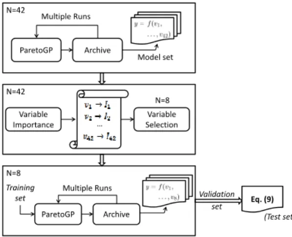
V. MODELINGPERCEIVEDVIDEOQUALITY This section presents the results of using GP-based symbolic regression to model the perceived video quality. First, all parameters extracted from the received video bitstream are made available to the modeling process. Next, based on the set of generated GP models, variable importance is determined. A new set of models is then generated using only the most important variables. Finally, from the resulting set of GP models, the best model is selected for predicting video quality. This approach is visually presented in Figure 6. This section is concluded by a comparison between the presented approach and other existing ML techniques. The performance of the metric is also validated on existing benchmark databases.
ParetoGP Archive Multiple Runs Model set N=42 Variable Importance … Variable Selection N=42 N=8 ParetoGP Archive Multiple Runs N=8 Training set Validation set Eq. (9) (Test set)
Fig. 6. Approach of using GP-based symbolic regression for estimating perceived video quality. After determining variable importance, a final set of candidate models is generated after which, the best model is selected for estimating video quality.
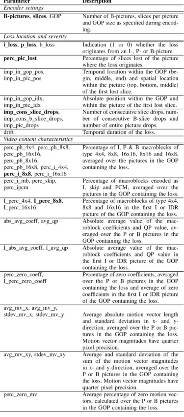
A. Listing of the parameters
The focus of this article is the construction of an NR bitstream-based objective video quality metric. Hence, only parameters that can be extracted or calculated from the re-ceived video bitstream, without the need for complete de-coding, are considered. This set comprisesN = 42different parameters that are subdivided into the following categories:
• Describe the encoder settings
• Identify the location and severity of the loss • Characterize the video content
A complete listing of the parameters is provided in Table III. Note that the parameter drift represents the temporal du-ration (extent) of the loss, i.e. the number of frames which are affected by the loss. If a loss occurs in an I-picture, the loss is propagated through the entire GOP. B-pictures are in our case never used as reference. Hence, losses in B-pictures only affect one picture and do not propagate any further. The temporal extent caused by losses in P-pictures depends on the location of that particular picture within the GOP. Based on our created video sequences (as detailed in Section IV-B), we calculated the average drift caused by losses in P-pictures, in relation to the position of that picture within the GOP. Hence, drift is calculated in the pixel domain as the number of pictures containing a visual distortion. The calculated values are listed in Table IV.
As indicated in Table III, all parameters are calculated based on the GOP containing the loss. If a loss occurs in an I-picture, statistics are calculated using the remaining P-and B-pictures. In case the loss occurs in a P-picture, the parameters are calculated using the I-picture and the remaining P-pictures in the GOP (except for the P-pictures where the loss originates from). This is similar when the loss originates from a B-picture, in which case the I- and B-pictures are used for calculating the statistics.
B. Identifying the importance of variables
First, all parameters are used during the modeling proce-dure, and the resulting set of models is shown in Figure 7.
TABLE III
OVERVIEW OF PARAMETERS EXTRACTED FROM RECEIVED VIDEO BITSTREAM IN ORDER TO IDENTIFY LOCATION OF LOSS AND TO CHARACTERIZE VIDEO CONTENT. THE SUBSET OF8INFLUENTIAL
PARAMETERS IS MARKED IN BOLD.
Parameter Description
Encoder settings
B-pictures,slices, GOP Number of B-pictures, slices per picture and GOP size as specified during encod-ing.
Loss location and severity
i loss,p loss, b loss Indication (1 or 0) whether the loss originates from an I-, P- or B-picture. perc pic lost Percentage of slices lost of the picture
where the loss originates. imp in gop pos,
imp in pic pos
Temporal location within the GOP (be-gin, middle, end) and spatial location within the picture (top, bottom, middle) of the first lost slice.
imp in gop idx, imp in pic idx
Absolute position within the GOP and within the picture of the first lost slice. imp cons slice drops,
imp cons b slice drops, imp pic drops
Number of consecutive slice drops, num-ber of consecutive B-slice drops and number of entire picture drops.
drift Temporal duration of the loss.
Video content characteristics perc pb 4x4, perc pb 8x8, perc pb 16x16,
perc pb 8x16,
perc pb 16x8, perc i 4x4, perc i 8x8, perc i 16x16
Percentage of I, P & B macroblocks of type 4x4, 8x8, 16x16, 8x16 and 16x8, averaged over the pictures in the GOP containing the loss.
perc i mb, perc skip, perc ipcm
Percentage of macroblocks encoded as I, skip and PCM, averaged over the pictures in the GOP containing the loss. I perc 4x4,I perc 8x8,
I perc 16x16
Percentage of macroblocks of type 4x4, 8x8 and 16x16 in the first I or IDR picture of the GOP containing the loss. abs avg coeff, avg qp Absolute average value of the
mac-roblock coefficients and QP value, av-eraged over the P or B pictures in the GOP containing the loss.
I abs avg coeff, I avg qp Absolute average value of the mac-roblock coefficients and QP value in the first I or IDR picture of the GOP containing the loss.
perc zero coeff, I perc zero coeff
Percentage of zero coefficients, averaged over the P or B pictures in the GOP containing the loss and average of zero coefficients in the first I or IDR picture of the GOP containing the loss. avg mv x, avg mv y,
stdev mv x, stdev mv y Average absolute motion vector length and standard deviation in x- and y-direction, averaged over the P or B pic-tures in the GOP containing the loss. Motion vector magnitudes have quarter pixel precision.
avg mv xy, stdev mv xy Average and standard deviation of the sum of the motion vector magnitudes in x- and y-direction, averaged over the P or B pictures in the GOP containing the loss. Motion vector magnitudes have quarter pixel precision.
perc zero mv Average percentage of zero motion
vec-tors, calculated over the P or B pictures in the GOP containing the loss.
Models that lie on the pareto front are marked in black and represent the best individuals in the population [46]. The plot illustrates that an increase in model complexity often results in more accurate predictions, and it shows that the model
TABLE IV
CALCULATED AVERAGE DRIFT(WITH STANDARD DEVIATION)CAUSED BY LOSSES INP-PICTURES,IN RELATION TO THE LOCATION WITHIN THE
GOPOF THEP-PICTURE. Location within GOP
BEGIN MIDDLE END
avg(drift) 14 9 4
stdev(drift) 1 2 2
prediction error saturates around 0.09. It is, however, found that variables which are not truly significant are often present in reasonable quantities in the final models. The presence of insignificant variables in regression models is usually unde-sired, because it can lead to overfitting and models that are very complex to interpret. There are multiple reasons why such variables can be present in models: due to the stochastic nature of the GP algorithm, insignificant variables that disappeared from models during the evolutionary run still have a chance to come back by means of the random mutation operator. On some occasions, insignificant variables are present in low-order metavariables evaluating to an important constant.
0 200 400 600 800 1000 0.10 1.00 0.50 0.20 0.30 0.15 0.70 Complexity 1 -R 2
Fig. 7. Set of GP models generated using all parameters extracted from the video bitstream. Models on the pareto front are marked in black.
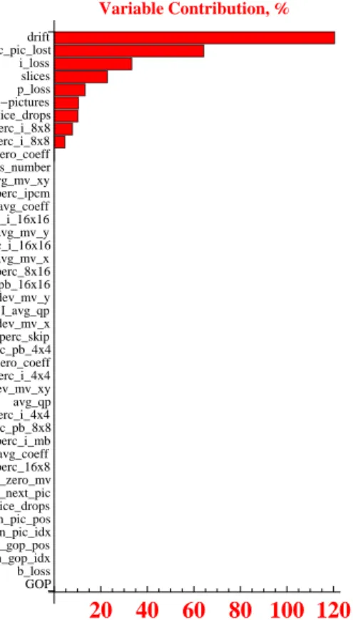
Fortunately, there is a robust way to overcome this problem. The DataModeler environment offers the variable contribu-tion analysis funccontribu-tion that estimates the contribucontribu-tion of each variable into the prediction error of each individual symbolic regression model, based on the rate of change in the relative prediction error when the variable is present or removed from the model. It estimates the contribution of each variable to each model in the set and aggregates all the results. Figure 8 demonstrates the quantitative characteristics of the variable contribution. E.g., a variable contribution of120%for variable
driftmeans that the removal of this variable from a model causes on average a 120% increase in the prediction error. This implies quantitatively that driftis a highly important variable, which clearly agrees with the common sense and domain knowledge. In order to determine the actual drift accurately, pixel data should be reconstructed. However, in this work, we are targeting a bitstream-based video quality metric which does not require a decoding (= pixel reconstruction) of the video stream. Therefore, it was decided to omit this parameter as well and to use only the parameters that can
exactly be extracted and calculated from the received encoded video bitstream. GOP b_loss imp_in_gop_idx imp_in_gop_pos imp_in_pic_idx imp_in_pic_pos imp_cons_b_slice_drops imp_drop_next_pic perc_zero_mv perc_16x8 abs_avg_coeff perc_i_mb perc_pb_8x8 perc_i_4x4 avg_qp stdev_mv_xy I_perc_i_4x4 I_perc_zero_coeff perc_pb_4x4 perc_skip stdev_mv_x I_avg_qp stdev_mv_y perc_pb_16x16 perc_8x16 avg_mv_x perc_i_16x16 avg_mv_y I_perc_i_16x16 I_abs_avg_coeff perc_ipcm avg_mv_xy ds_number perc_zero_coeff perc_i_8x8 I_perc_i_8x8 imp_cons_slice_drops B-pictures p_loss slices i_loss perc_pic_lost drift
20
40
60
80 100 120
Variable Contribution,%Fig. 8. Contribution of each variable into the prediction error of the regression models when removing that particular variable from the model.
The results of the variable contribution analysis show that there areN = 8influential parameters for modeling perceived video quality: perc_pic_lost, i_loss, slices,
p_loss, B_pictures, imp_cons_slice_drops,
I_perc_8x8 and perc_i_8x8. Interestingly, these parameters largely correspond with the variables that were used in our previous work [33] for modeling the impairment visibility in H.264/AVC encoded HD video sequences.
C. Final modeling of Perceived Quality
The variable contribution analysis is most beneficial, since it identifies that only 20% of video bitstream parameters are causing significant changes in the video quality perception. This information is of high value because it significantly decreases the problem dimensionality, and focuses future research. In this section, a final modeling step is applied to construct an objective quality metric using only the most important variables as determined in the previous section.
In order to compute an interpretable model that uses only these influential variables, the data set S is divided into a disjoint training (60%), validation (20%) and test (20%) set. The training setis used to generate new models based on the subset of 8 parameters and the results are depicted in Figure 9. It shows that the models are able to fit the data using much less variables without suffering a significant loss in accuracy. All models that lie on the pareto front are now candidate models for predicting video quality. In order to pick the “best”
0 200 400 600 800 1000 1.00 0.50 0.20 0.30 0.15 0.70 Complexity 1 -R 2
Fig. 9. Set of GP models generated using only the selected influential parameters. Models on the pareto front are marked in black.
20 40 60 80 100 120 0.0 0.2 0.4 0.6 0.8 1.0 Complexity :1 R 2
Fig. 10. Prediction error versus model complexity for each pareto efficient model identified using the validation set. The arrow indicates the final selected model.
model from the set, all pareto-optimal models in Figure 9 are evaluated on thevalidation set. Figure 10 plots the prediction error between predicted and actual MOS against model’s complexity for each pareto optimal models evaluated on the
validation set. Model complexity is computed as the total sum of nodes in all the subtrees of the parse tree representation of that particular model. In order to select the final model, a trade-off must be made between model complexity and accuracy. Based on the plot in Figure 10, it can be seen that the performance saturates of the pareto optimal models with a complexity of 60 or more. Therefore, we selected the final model (indicated by the arrow in Figure 10) as the point in the graph after which there is no significant gain in prediction accuracy. This corresponds with the point located near the ‘elbow’ of the plot.
The performance of the final model is then assessed by evaluating it over the test setthat contains previously unseen data. For each data sample in the test set, the predicted MOS (M OSp) is compared to the actual MOS (q) and the result is depicted in Figure 11. The Pearson correlation coefficient R
over the test set is 0.9003 with a Root Mean Squared Error (RMSE) of 0.5663, which confirms that the final model is indeed capable of predicting perceived quality with a high accuracy, using only a limited number of parameters extracted
2 3 4 5 2 3 4 5 Observed Predicted
Fig. 11. Predicted MOS (eq. 9) versus actual MOS over the test set.
solely from the received encoded video bitstream.
D. Objective Video Quality Metric
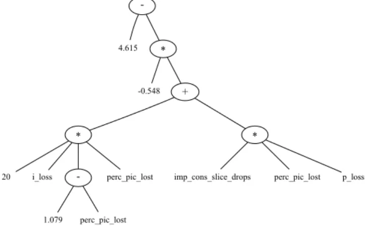
The parse tree corresponding with the final selected model is depicted in Figure 12. This tree can easily be translated to the algebraic expression shown in equation (9) that is shown on top of the next page. In this model, only four
-4.615 * -0.548 + * * 20 i_loss - perc_pic_lost 1.079 perc_pic_lost
imp_cons_slice_drops perc_pic_lost p_loss
Fig. 12. Parse tree corresponding with the selected GP model indicated in Figure 10.
parameters are present for estimating video quality, since only models with a higher complexity use all eight parameters. This formula computes the predicted MOS as a large constant from which multiple terms are subtracted. Each term is weighted by the type of picture where the loss originates from. Losses originating in I- or P-pictures cause a drop in perceived quality. In the case losses occur in B-pictures, perceived quality equals 4.615. In previous research [33], we found that losses in B-pictures are never perceived. As such, the quality is not influenced. The fact that, in this case, perceived quality does not equal 5 (i.e. ‘excellent’ quality) can be explained by the fact that subjects tend to avoid using the extremes of the rating scales [47] during the subjective video quality evaluation. This effect is also known as the saturation effect[48].
In general, losses in I-pictures will result in a higher drop in quality due to the drift (=spatial extent) caused by the decoding
dependencies with other pictures in the GOP. Losses of entire I-pictures are rated higher quality compared to losing only a certain portion of the picture. This matches the conclusions of [33] where it was found that dropping an entire picture and relying on the error concealment strategy might benefit quality perception. In the case of similar consecutive pictures, frame freezes can be used as an efficient concealment technique [49]. When losses originate from P-pictures, the drop in perceived quality is further depending on the amount of slices per picture and the amount of slices lost. For the same amount of the picture lost (perc_pic_lost), a higher number of slices per picture will result in a slightly higher drop in quality. This again matches with the earlier findings [33] that impairment visibility of loosing up to half a picture depends on the number of encoded slices in that particular picture, i.e. impairments are easier detected in sequences encoded with multiple slices.
E. Performance comparison
In this last section, the results of the GP-based symbolic regression approach are compared to several state-of-the-art ML techniques. To this end, the same training, validation and test set are used as in the previous section. Two different model types are investigated and the results are listed in Table V:
• The first model type is a two-layer feed-forward Artificial Neural Network (ANN) with sigmoid hidden neurons and linear output neurons. It is found that this network topology is able to approximate the non-linear function
f(~v)sufficiently well. Based on experimental results, the number of neurons in the hidden layer is set to 4 and the weights of the neural network are computed with the Levenberg-Marquardt backpropagation algorithm [50]. • The second model type is the Support Vector Regression
(SVR) model used by Narwariaet al.[27]. Each attribute of the input vector~vis scaled to [0,1] and the following model is computed, f(~v) = k X i=1 (α∗i −αi)K(~vi, ~v) +b (10) where K is chosen to be a radial basis function kernel that maps the problem from a lower dimensional space to a higher feature space andb is a real constant.
K(~vi, ~v) = exp(−γk~vi−~vk2),γ >0 (11) The variablesαi andα∗i are optimized by maximizing a constrained quadratic function, and the constantsγandC
are selected from a grid of increasing values. The reader is referred to [51] for a detailed discussion of the algorithm. As can be seen from Table V, the accuracy of the GP-based symbolic regression metric (see equation 9) yields perfor-mance results that are comparable to, or better than the ANN and SVR algorithms. A key advantage of the GP approach is that it provides a natural way for variable selection and yields interpretable models. Discarding redundant variables is important, as it reduces the dimensionality of the problem. Numerical results in Table V confirm that models which are based on the subset of 8 (or even 4) parameters are indeed sufficiently accurate to characterize the perceived quality.
M OSp= 4.615−0.548·(20·i loss·(1.079−perc pic lost)·perc pic lost+imp cons slice drops·perc pic lost·p loss) (9) TABLE V
PEARSONLINEARCORRELATIONCOEFFICIENT(PLCC), SPEARMANRANK-ORDERCORRELATIONCOEFFICIENT(SROCC)ANDPREDICTION ERROR 1−R2USING DIFFERENT MODEL TYPES
Training Validation Test All
Model type PLCC SROCC Error PLCC SROCC Error PLCC SROCC Error PLCC SROCC Error
GP metric (4) 0.9047 0.75107 0.1814 0.8619 0.8288 0.2571 0.9003 0.8447 0.1895 0.8961 0.7961 0.1969 ANN (42) 0.9680 0.9164 0.0629 0.8975 0.8827 0.1945 0.8551 0.8363 0.2688 0.9310 0.8990 0.1333 ANN (8) 0.9330 0.8522 0.1294 0.8540 0.8284 0.2707 0.8712 0.8115 0.2411 0.9057 0.8447 0.1797 ANN (4) 0.9111 0.7829 0.1699 0.8567 0.8330 0.2661 0.8931 0.8231 0.2023 0.8977 0.8077 0.1941 SVR (42) 0.9665 0.9341 0.0660 0.9159 0.8746 0.1612 0.9270 0.8829 0.1407 0.9486 0.9076 0.1002 SVR (8) 0.9225 0.8489 0.1490 0.8590 0.8390 0.2621 0.9012 0.8394 0.1879 0.9065 0.8489 0.1783 SVR (4) 0.9107 0.7959 0.1706 0.8609 0.8202 0.2588 0.8713 0.8188 0.2408 0.8946 0.8089 0.1998
When providing all available parameters to the modeling process, the SVR model achieves a slightly higher accuracy. However, this requires an in-depth processing of the received video stream. This, in turn, increases model complexity. In the case of real-time monitoring, models using parameters which do not require in-depth processing are preferred.
F. Model validation
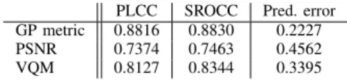
The validity of the proposed metric (9) has also been checked by applying it to the publicly available EPFL-PoliMI video quality assessment database [52], [53]. This database contains, 72 4CIF resolution (704x576 pixels) and 72 CIF resolution H.264/AVC encoded video sequences impaired at different packet loss rates. The MOS scores which are pre-dicted by our metric (see Equation 9) are compared to the MOS scores in the database, and the PLCC, the SROCC and the prediction error (1−R2) are computed. The performance of our metric is also compared against two well known FR quality metric, namely PSNR and VQM [23], for benchmarking.
TABLE VI
PERFORMANCE EVALUATION OF OUR PROPOSED METRIC, PSNRAND
VQMAGAINST THEEPFL-POLIMIVIDEO DATABASE.
PLCC SROCC Pred. error
GP metric 0.8816 0.8830 0.2227
PSNR 0.7374 0.7463 0.4562
VQM 0.8127 0.8344 0.3395
It is seen from Table VI that the metric yields a very good agreement, which confirms that the metric has good generalization properties and that it also works well on similar video sequences. Comparing the performance of our metric against PSNR and VQM measurements show that our NR bitstream-based metric achieves a higher accuracy in estimat-ing perceived quality.
VI. CONCLUSION
In this article, a novel machine learning technique for con-structing a no-reference bitstream-based objective video qual-ity metric is proposed. Genetic programming-based symbolic
regression is used to generate sets of white box models for estimating perceived quality. This, in turn, yields interpretable models and allows automatic selection of the most quality-affecting parameters. The modeling technique does not make any a priori assumptions on the functional form or the com-plexity of the final model(s). Since the focus of the article is a no-reference bitstream-based metric, only parameters which can be extracted from the received encoded video bitstream without the need for complete decoding are taken into account during the modeling process.
In total, 42 different parameters are extracted from the bitstream characterizing the encoding settings, the type of loss and the video content. Based on the variable contribution analysis of the modeling toolkit, it is found that only 20% of these parameters significantly influence perceived quality. Modeling results confirm that the perceived quality can be estimated accurately using only a very limited number of pa-rameters. This enables real-time no-reference-based objective video quality monitoring for video service providers.
ACKNOWLEDGMENT
The research activities that have been described in this paper were funded by Ghent University, iMinds and the Institute for the Promotion of Innovation by Science and Technology in Flanders (IWT). This paper is the result of research carried out as part of the OMUS project funded by the iMinds. OMUS is being carried out by a consortium of the industrial partners: Technicolor, Televic, Streamovations and Excentis in coopera-tion with iMinds research groups: IBCN & MultimediaLab & WiCa (UGent), SMIT (VUB), PATS (UA) and COSIC (KUL). This work was also supported by the Research Foundation in Flanders (FWO-Vlaanderen). Dirk Deschrijver is a post-doctoral research fellow of FWO-Vlaanderen.
REFERENCES
[1] N. Staelens, S. Moens, W. Van den Broeck, I. Mari¨en and, B. Vermeulen, P. Lambert, R. Van de Walle, and P. Demeester, “Assessing quality of experience of IPTV and Video on Demand services in real-life environments,”IEEE Transactions on Broadcasting, vol. 56, no. 4, pp. 458–466, December 2010.
[2] N. Staelens, K. Casier, W. Van den Broeck, B. Vermeulen, and P. De-meester, “Determining customer’s willingness to pay during in-lab and real-life video quality evaluation,” Sixth International Workshop on Video Processing and Quality Metrics for Consumer Electronics (VPQM-12), January 2012.
[3] G. Cermak, “Consumer Opinions About Frequency of Artifacts in Digital Video,”IEEE Journal of Selected Topics in Signal Processing, vol. 3, no. 2, pp. 336 –343, April 2009.
[4] DSL Forum Technical Report TR-126, “Triple-play Services Quality of Experience (QoE) requirements,” DSL Forum, 2006.
[5] M. Pinson and S. Wolf, “Comparing subjective video quality testing methodologies,” T. Ebrahimi and T. Sikora, Eds., vol. 5150, no. 1. SPIE, 2003, pp. 573–582.
[6] ITU-T Recommendation P.910, “Subjective video quality assessment methods for multimedia applications,” International Telecommunication Union (ITU), 1999.
[7] ITU-R Recommendation BT.500, “Methodology for the subjective as-sessment of the quality of television pictures,” International Telecom-munication Union (ITU), 2009.
[8] Z. Wang, H. R. Sheikh, and A. C. Bovik, “Objective video quality assess-ment,” inThe Handbook of Video Databases: Design and Applications, B. Furht and O. Marqure, Eds. CRC Press, 2003, pp. 1041–1078. [9] ITU-T Recommendation J.341, “Objective perceptual multimedia video
quality measurement of HDTV for digital cable television in the pres-ence of a full referpres-ence,” International Telecommunication Union (ITU), 2011.
[10] ITU-T Recommendation J.342, “Objective multimedia video quality measurement of HDTV for digital cable television in the presence of a reduced reference signal,” International Telecommunication Union (ITU), 2011.
[11] M. Naccari, M. Tagliasacchi, and S. Tubaro, “No-reference video quality monitoring for H.264/AVC coded video,”IEEE Transactions on Multimedia, vol. 11, no. 5, pp. 932 – 946, August 2009.
[12] S. Chikkerur, V. Sundaram, M. Reisslein, and L. J. Karam, “Objective video quality assessment methods: A classification, review, and perfor-mance comparison,”IEEE Transactions on Broadcasting, 2011. [13] Video Quality Experts Group (VQEG), “Final report from the
Video Quality Experts Group on the validation of objective models of video quality assessment, Phase II,” August 2003. [Online]. Available: http://www.its.bldrdoc.gov/vqeg/project-pages/frtv-phase-ii/frtv-phase-ii.aspx
[14] ——, “Final Report of VQEGs Multimedia Phase
I Validation Test,” September 2008. [Online].
Avail-able: http://www.its.bldrdoc.gov/vqeg/project-pages/multimedia-phase-i/multimedia-phase-i.aspx
[15] ——, “Report on the Validation of Video Quality Models for High Definition Video Content,” June 2010. [Online]. Available: http://www.its.bldrdoc.gov/vqeg/projects/hdtv/
[16] S. Mohamed, G. Rubino, H. Afifi, and F. Cervantes, “Real-time video quality assessment in packet networks: A neural network model,” in Proceedings of the International Conference on Parallel and Distributed Processing Techniques and Applications, June 2001.
[17] S. Mohamed and G. Rubino, “A study of real-time packet video quality using random neural networks,” IEEE Transactions on Circuits and Systems for Video Technology, vol. 12, no. 12, pp. 1071 – 1083, December 2002.
[18] J. Choe, K. Lee, and C. Lee, “No-reference video quality measurement using neural networks,” in 16th International Conference on Digital Signal Processing, July 2009, pp. 1 –4.
[19] P. Gastaldo, S. Rovetta, and R. Zunino, “Objective quality assessment of MPEG-2 video streams by using cbp neural networks,”IEEE Trans-actions on Neural Networks, vol. 13, no. 4, pp. 939 –947, July 2002. [20] P. Le Callet, C. Viard-Gaudin, and D. Barba, “A convolutional neural
network approach for objective video quality assessment,”IEEE Trans-actions on Neural Networks, vol. 17, no. 5, pp. 1316 –1327, September 2006.
[21] H. El Khattabi, A. Tamtaoui, and D. Aboutajdine, “Video quality assessment measure with a neural network,” International Journal of Computer and Information Engineering, vol. 4, no. 3, pp. 167 – 171, 2010.
[22] B. Wang, D. Zou, and R. Ding, “Support vector regression based video quality prediction,” in IEEE International Symposium on Multimedia (ISM), December 2011.
[23] ITU-T Recommendation J.144, “Objective perceptual video quality measurement techniques for digital cable television in the presence of a full reference,” International Telecommunication Union (ITU), 2004.
[24] N. Narvekar, T. Liu, D. Zou, and J. Bloom, “Extending G.1070 for video quality monitoring,” in IEEE International Conference on Multimedia and Expo (ICME), July 2011, pp. 1 –4.
[25] M. Narwaria and W. Lin, “Machine learning based modeling of spatial and temporal factors for video quality assessment,” in International Conference on Image Processing, vol. 1, September 2011, pp. 2513 –2516.
[26] M. Narwaria, W. Lin, and L. Anmin, “Low-complexity video quality assessment using temporal quality variations,” IEEE Transactions on Multimedia, vol. 14, no. 3, pp. 525 –535, June 2012.
[27] M. Narwaria and W. Lin, “Svd-based quality metric for image and video using machine learning,” IEEE Transactions on Systems, Man, and Cybernetics - Part B: Cybernetics, vol. 42, no. 2, pp. 347 –364, April 2012.
[28] S. Argyropoulos, A. Raake, M.-N. Garcia, and P. List, “No-reference bit stream model for video quality assessment of h.264/avc video based on packet loss visibility,” inIEEE International Conference onAcoustics, Speech and Signal Processing (ICASSP), May 2011, pp. 1169 –1172. [29] S. Argyropoulos, A. Raake, M. Garcia, and P. List, “No-reference
video quality assessment for sd and hd h.264/avc sequences based on continuous estimates of packet loss visibility,” in Third International Workshop on Quality of Multimedia Experience (QoMEX), September 2011, pp. 31 –36.
[30] A. Reibman, S. Kanumuri, V. Vaishampayan, and P. Cosman, “Visi-bility of individual packet losses in MPEG-2 video,” inInternational Conference on Image Processing, vol. 1, October 2004, pp. 171–174. [31] S. Kanumuri, P. Cosman, A. Reibman, and V. Vaishampayan,
“Mod-eling packet-loss visibility in MPEG-2 video,”IEEE Transactions on Multimedia, vol. 8, no. 2, pp. 341–355, April 2006.
[32] V. Menkovski, G. Exarchakos, and A. Liotta, “Machine learning ap-proach for quality of experience aware networks,” in2nd International Conference on Intelligent Networking and Collaborative Systems (IN-COS), November 2010, pp. 461 –466.
[33] N. Staelens, G. Van Wallendael, K. Crombecq, N. Vercammen, J. De Cock, B. Vermeulen, R. Van de Walle, T. Dhaene, and P. De-meester, “No-Reference Bitstream-based Visual Quality Impairment Detection for High Definition H.264/AVC Encoded Video Sequences,” IEEE Transactions on Broadcasting, vol. 58, no. 2, pp. 187–199, June 2012.
[34] K. Vladislavleva, K. Veeramachaneni, M. Burland, J. Parcon, and U.-M. O’Reilly, “Knowledge mining with genetic programming methods for variable selection in flavor design,” inProceedings of the 12th annual conference on Genetic and evolutionary computation, ser. GECCO ’10. ACM, 2010, pp. 941–948.
[35] P. Gastaldo and J. A. Redi, “Machine learning solutions for objective visual quality assessment,” Sixth International Workshop on Video Processing and Quality Metrics for Consumer Electronics (VPQM-12), January 2012.
[36] Evolved Analytics LLC, DataModeler Release 8.0 Documentation. Evolved Analytics LLC, 2010. [Online]. Available: www.evolved-analytics.com
[37] J. R. Koza,Genetic Programming: On the Programming of Computers by Means of Natural Selection, ser. A Bradford Book. Cambridge Mass, London: The MIT Press, 1992.
[38] M. Pinson, S. Wolf, N. Tripathi, and C. Koh, “The consumer digital video library,” Fifth International Workshop on Video Processing and Quality Metrics for Consumer Electronics (VPQM-10), January 2010. [39] G. E. Legge and J. M. Foley, “Contrast masking in human vision,”
Journal of the Optical Society of America, vol. 70, no. 12, pp. 1458– 1471, Dec 1980.
[40] Y. Zhong, I. Richardson, A. Sahraie, and P. McGeorge, “Influence of task and scene content on subjective video quality,” inImage Analysis and Recognition, ser. Lecture Notes in Computer Science, A. Campilho and M. Kamel, Eds. Springer Berlin / Heidelberg, 2004, vol. 3211, pp. 295–301.
[41] A. Ostaszewska and R. Kloda, “Quantifying the amount of spatial and temporal information in video test sequences,” inRecent Advances in Mechatronics. Springer Berlin Heidelberg, 2007, pp. 11–15. [42] G. O’Driscoll,Next Generation IPTV Services and Technologies. New
York, NY, USA: Wiley-Interscience, 2008.
[43] A. Rombaut, N. Staelens, N. Vercammen, B. Vermeulen, and P. De-meester, “xStreamer: Modular Multimedia Streaming,” inProceedings of the seventeenth ACM international conference on Multimedia, 2009, pp. 929–930.
[44] N. Staelens, N. Vercammen, Y. Dhondt, B. Vermeulen, P. Lambert, R. Van de Walle, and P. Demeester, “ViQID: A no-reference bit stream-based visual quality impairment detector,” in Second International
Workshop on Quality of Multimedia Experience (QoMEX), June 2010, pp. 206 –211.
[45] N. Staelens and G. Van Wallendael, “Adjusted JM Reference Software 16.1 with XML Tracefile Generation Capabilities,” VQEQ JEG Hybrid 2011 029 jm with xml tracefile v1.0, Hillsboro, Oregon, US, December 2011.
[46] G. Smits and F. Kotanchek, Pareto-Front Exploitation in Symbolic Regression, ser. Genetic Programming Theory and Practice II. Springer, 2004, ch. 17, pp. 283–299.
[47] P. Corriveau, Video Quality Testing, ser. Digital Video Image Quality and Perceptual Coding. CRC Press, 2006, ch. 4, pp. 125–153. [48] Q. Huynh-Thu, M.-N. Garcia, F. Speranza, P. Corriveau, and A. Raake,
“Study of rating scales for subjective quality assessment of high-definition video,”IEEE Transactions on Broadcasting, vol. 57, no. 1, pp. 1–14, march 2011.
[49] N. Staelens, B. Vermeulen, S. Moens, J.-F. Macq, P. Lambert, R. Van de Walle, and P. Demeester, “Assessing the influence of packet loss and frame freezes on the perceptual quality of full length movies,”Fourth International Workshop on Video Processing and Quality Metrics for Consumer Electronics (VPQM-09), January 2009.
[50] B. Sch¨olkopf and A. J. Smola,Learning with Kernels: Support Vector Machines, Regularization, Optimization, and Beyond. MIT Press, 2002. [51] S. Haykin,Neural Networks. Prentice Hall, 1999.
[52] F. De Simone, M. Naccari, M. Tagliasacchi, F. Dufaux, S. Tubaro, and T. Ebrahimi, “Subjective assessment of H.264/AVC video sequences transmitted over a noisy channel,” inFirst International Workshop on Quality of Multimedia Experience (QoMEX), July 2009, pp. 204 –209. [53] F. De Simone, M. Tagliasacchi, M. Naccari, S. Tubaro, and T. Ebrahimi, “A H.264/AVC video database for the evaluation of quality metrics,” in IEEE International Conference on Acoustics Speech and Signal Processing (ICASSP), March 2010, pp. 2430 –2433.
Nicolas Staelens obtained his Master’s degree in Computer Science at Ghent University (Belgium, 2004). He started his career in 2004 as an R&D engineer at Televic (a Belgian company that de-velops, designs and manufactures high-end network systems and software applications for the healthcare market). In 2006, he joined the IBCN-group (Inter-net Based Communication Networks and Services) at Ghent University - iMinds as a Ph.D. student. His research focuses on studying the effects of network impairments on the perceived quality of audiovisual sequences. As of 2007, he is also actively participating within the Video Quality Experts Group (VQEG) and is currently co-chair of the Tools and Subjective Labs support group and the JEG-Hybrid project.
Dirk Deschrijver was born in Tielt, Belgium, on September 26, 1981. He received the Masters (Li-centiaat) degree and the PhD degree in Computer Science from the University of Antwerp, Antwerp, Belgium, in 2003 and 2007 respectively. From May to October 2005, he was a Marie Curie Fellow with the Scientific Computing Group, Eindhoven Univer-sity of Technology, Eindhoven, The Netherlands. He is currently an FWO Post-Doctoral Research Fellow with the Department of Information Technology (INTEC), iMinds, Ghent University, Gent, Belgium. His research interests include robust parametric macromodeling, rational least squares approximation, orthonormal rational functions, system identification, and broadband macromodeling techniques.
Ekaterina (Katya) Vladislavlevais a Chief Data Scientist and Partner at Evolved Analytics and co-owner of Evolved Analytics Europe. She did a PhD on symbolic regression at Tilburg University, the Netherlands. Katya also holds a Professional Doctor-ate in Engineering (in industrial mathematics) from Eindhoven University of Technology, the Nether-lands, and a Master of Science in Mathematics (in mathematical theory of intelligent systems) from Moscow State University of Lomonosov, Moscow, Russia. Katya pursues research in data-driven mod-eling, high-performance computing, and industrial optimization, particularly in the industrial scale data analysis and predictive modeling for process and research analytics.
Brecht Vermeulenreceived his Electronic Engineer-ing degree in 1999 from Ghent University, Belgium. In June 2004, he received his Ph.D. degree for the work entitled “Management architecture to support quality of service in the internet based on IntServ and DiffServ domains” at the Department of Infor-mation Technology of Ghent University. Since June 2004, he leads a research team within the IBCN group led by Prof. Demeester which investigates network and server performance and quality of expe-rience in the fields of video, audio/voice and multiple play. Since the start iMinds in 2004, he also leads the iMinds Technical Test Centre in Ghent, Belgium.
Tom Dhaene (M1794, SM1705) was born in Deinze, Belgium, on June 25, 1966. He received the Ph.D. degree in electrotechnical engineering from the University of Ghent, Ghent, Belgium, in 1993. From 1989 to 1993, he was Research Assistant at the University of Ghent, in the Department of Information Technology, where his research focused on different aspects of full-wave electro-magnetic circuit modeling, transient simulation, and time-domain characterization of frequency and high-speed interconnections. In 1993, he joined the EDA company Alphabit (now part of Agilent). He was one of the key developers of the planar EM simulator ADS Momentum. Since September 2000, he has been a Professor in the Department of Mathematics and Computer Science at the University of Antwerp, Antwerp, Belgium. Since October 2007, he is a Full Professor in the Department of Information Technology (INTEC) at Ghent University, Ghent, Belgium. As author or co-author, he has contributed to more than 220 peer-reviewed papers and abstracts in international conference proceedings, journals and books.
Piet Demeester is professor in the faculty of En-gineering at Ghent University. He is head of the research group “Internet Based Communication Net-works and Services” (IBCN) that is part of the Department of Information Technology (INTEC) of Ghent University. He is also leading the Future Internet (Networks, Media and Service) Department of iMinds. He is Fellow of the IEEE.