Variable Interactions in Risk Factors for Dementia
Jim O’ Donoghue, Mark Roantree & Andrew McCarren
Insight Centre for Data Analytics School of Computing Dublin City University
Glasnevin, Dublin 9 Ireland
Email:{jodonoghue, mroantree, amccarren}@computing.dcu.ie
Abstract—Current estimates predict 1 in 3 people born today will develop dementia, suggesting a major impact on future population health. As such, research needs to connect specialist clinicians, data scientists and the general public. The In-MINDD project seeks to address this through the provision of aProfiler, a socio-technical information system connecting all three groups. The public interact, providing raw data; data scientists develop and refine prediction algorithms; and clinicians use in-built services to inform decisions. Common across these groups are Risk Factors, used for dementia-free survival prediction. Risk interactions could greatly inform prediction but determining these interactions is a problem underpinned by massive numbers of possible combinations. Our research employs a machine learning approach to automatically select best performing hyper-parameters for prediction and learns variable interactions in a non-linear survival-analysis paradigm. Demonstrating effective-ness, we evaluate this approach using longitudinal data with a relatively small sample size.
I. INTRODUCTION
In 2014, the UK Alzheimer’s Society published a major study on the social and economic impact of dementia in the UK. The report projected that 850,000 people would be living with dementia in the UK by 2015, with associated costs of£26 billion a year [8]. Furthermore, a European study published in 2013 [7] cited the average rate of dementia across 28 countries to be 1.55% of the population. These studies point to dementia as one of the greatest health risks to society today. As a result, systems are required that connect experts from different disciplines to each other, as well as to their target group in society. The In-MINDD project [4], delivers this through the development of the In-MINDD Profiler, a socio-technical information system which requires multi-disciplinary collaboration between experts in the field of dementia, IT researchers and support staff in order to provision members of society most at risk with state-of-the-art tools for dementia prediction and mitigation.
A. The In-MINDD System
The goal of the In-MINDD project is to develop and validate online tools for middle-aged (40-60) individuals which assess lifestyle factors and how these affect long term brain health, provide personalised strategies for adopting a brain healthy lifestyle and present online supports to help participants im-plement and adhere to positive change in order to lower the risk of developing dementia. This requires knowledge building
and knowledge sharing, with system-driven decision making, across heterogeneous cultures and health systems.
The development and validation of an online dementia as-sessment tool requires close collaboration of clinical dementia experts and data scientists. The first element of developing this online system required the definition of a common vocabulary or ontology, in order to share knowledge between relevant stakeholders [18], [19]. Next a multi-factorial model of those elements that pertained to dementia-risk in middle-aged indi-viduals was developed by dementia experts via a systematic literature review [6] and shared with the data scientists via the previously defined system ontology [18], [19]. The system ontology connects the IT and clinical researchers and allows both parties to validate the model - data scientists via the latest machine learning techniques and clinical researchers through more traditional statistical approaches. The result of this work was incorporated into a prototype model for inclu-sion in the Profiler which was developed by the computing researchers. The Profiler presents a user with a series of questions, evaluates the answers to these and hence, provides a brain-health score. Subsequently, the Profiler presents the participant with a series of goals to improve their brain-health and mitigate against those factors from which they are most at risk. This is fundamentally different to systems such as that described in [17] where data is automatically generated in a uniform manner by purpose-built devices. The In-MINDD project is now testing this prototype model to assess if a 6 month intervention with the online profiler and support environment can improve the level of dementia risk in those most susceptible [14].
The previously defined information-system allows iterations and inclusions of improvements in the model, which is the focus of this work. The aim is to improve the predictive power of the model, through machine learning algorithms that offer deeper analyses compared to traditional statistical approaches and can identify latent classes over the course of learning, resulting in candidate risk-factor interactions. These interactions cannot be assessed by data scientists, instead results will be provided to dementia experts for an informed clinical evaluation.
B. Problem Statement and Motivation
As stated in Section I-A, early in the In-MINDD project, dementia researchers identified the 14 most prevalent risk factors from published research which can be used to measure a person’s risk of developing dementia [6]. With the exception of age, gender, and years of education, the remaining 11 risk factors are modifiable, meaning if clinical researchers can determine strong risk factors and have the person involved modify their behaviour, they can reduce their likelihood of developing dementia. These modifiable risk factors were iden-tified as cognitive activity,physical activity, mid-life obesity, diabetes,moderate alcohol use (protective),smoking, depres-sion,mid-life hypertension,cholesterol,cardiovascular disease andkidney disease. It is necessary for researchers to determine how these variables interact in order to build an optimum predictive model for identifying and extending life without dementia in middle-aged individuals. For clinical researchers, finding these interactions is a significant task using statistical software packages due to the high number of permutations involved. There is also a need to develop an a-priori hypothesis of interactions before testing these in a relevant dataset.
This motivates the need to obtain a deeper understanding of the interactions between risk factors. Neural networks provide possibilities to measure these interactions through examining thelatentfeatures found in their hidden layers and the weights that combine the visible variables to make up these hidden features. By latentfeatures, we mean thoseabstractvariables that combine more fine-grained variables into higher-level attributes we are trying to determine. The weights which are the coefficients for the input features are the outputs of our experiments, described in Section IV. The main problem dealt with here is detecting the appropriate latent variables from the very high number of potential multi-attribute combinations that exist and adopting a non-linear dementia survival analysis in the process.
The ideal dataset for this type of research is a longitudi-nal study which tracks behaviour over a number of years, preferably for those in middle-age. The dataset used was the Maastricht ageing study (MAAS dataset) [3] which was generated from a longitudinal, prospective cohort study which recorded lifestyle and biometric data on middle-aged individ-uals through 86 types of tests at 3 year intervals over more than 12 years.
C. Contribution
Consider that we have a system in place that connects clinical researchers with participants in a study trial. For this system the data scientist must also access further study trial data to provide a deeper analysis and determine how risk factors interact in the highest performing predictive model, subsequently presenting these risk interactions to the clinical researchers. Our primary contribution is in the construction of neural network models for a set of seven tests to determine the best performing of 14 different predictive models for survival analysis. Each model involved a separate experimental run of 512 test configurations, in each case risk interactions were
learned and the weights for each combination of interactions were recorded, to enable the optimal configuration to be found. D. Paper Structure
The remainder of this paper is structured as follows: in Section II, we describe our approach as a 2-step process of parameter set-up and optimisation; in Section III, we discuss how our system is configured and the different dataset types that served as input; our evaluation, results and analysis are described in Section IV; in Section V, we contrast our work with similar efforts in this area while in Section VI, we provide some conclusions.
II. APPROACH
Two aims are to be solved with our approach: to determine multi-variate feature interactions in dementia survival analysis; and to adopt a non-linear approach as many participants in the Maas dataset have similar attributes but different classi-fications. Non-linear analyses better model these participant differences and thus, provide superior accuracy in outcome predictions. We use a Multi-Layer Perceptron (MLP) to per-form supervised classification and our approach tackles one of the 10 challenges [21] in data mining research: data mining for biological problems.
Supervised classification is a machine learning paradigm which trains an algorithm on data in order to predict a particular outcome; in our case, we perform multi-class clas-sification to distinguish between survival cases and those who encountered dementia, death or censorship (study drop-out) in the dataset. An MLP is an artificial neural network (ANN) that learns abstract features from the data. We hypothesise that these abstract features model the complex dementia risk factor interactions to better predict the outcomes in question. Our approach builds on the outline platform developed in [16] [15], with a new 2-step process to deliver high performing prediction models.
A. Step 1: Determine Hyper-Parameter Settings
The broad purpose of Step 1 is to determine the hyper-parameters for all experiments. Before this step, we have a set of bounds for each hyper-parameter and after this step, all hyper-parameter configurations will be determined (Section III-B elaborates on this).Hyper-parametersare algorithm tuning-parameters that influence how model weights are learned in training according to the optimisation procedure outlined in III-B. The number of hidden layer nodes and learning rate (parameter for magnitude of weight updates) are examples. This must be completed before any form of model optimisation can begin.
B. Step 2: Hyper-Parameter Optimisation
There are five separate procedures in Step 2 that are repeated for each of the 256 trials, for each experiment combination described in Section III-A.
1) Initialise Architecture: This process uses a hyper-parameter configuration from Step 1 to generate the appro-priate algorithm configuration and architecture, setting the number of nodes and layers, inputs and outputs, associating all relevant hyper-parameters to the configuration and initialising relevant weights and biases.
2) Construct Hypothesis: Thehypothesis_function
combines the model weights with each sample of dataset variables and incorporates the appropriate activation and clas-sification functions that allow for making predictions. We used an MLP with one hidden layer.
zj(0)=b(0)j + n X i=1 xiw (0) ij (1) P(nj= 1|x, θ(0)) =aj= 1 1 +e−z (0) j (2) zk(1)= m X j=1 ajw (1) jk (3) P(yk= 1|x, θ) = ez(1)k K P k=1 ez(1)k (4)
Equations 1 and 2 are the functions between the input to hiddenlayers and Equations 3 and 4 are thehiddento classifi-cationlayer functions. The parametersθ(0)for the input to
hid-den layers are{b(0), W(0)}the bias and weights respectively.
Equivalently, {b(1), W(1)} are the parameters for the hidden
to output layers θ(1). The complete set of these parameters
{θ(0), θ(1)}are denotedθ.xis the set of input feature values from1. . . mwheremis the total number of features.nis the set of hidden nodes anda are the activations for these nodes from 1. . . o, the total number of nodes in the hidden layer. k refers to a particular classification in the range of output classes 1. . . K. For Equation 1, weights are multiplied by the input features to give a linear combination before entering the non-linear logistic sigmoid activation function -Equation 2 - to compute the probabilities of a hidden node n being ’on’ or ’off’ - also known as a node’s activation energy. This is the point where we hypothesise interactions are found for the input variables, as during training, each hidden node learns different combinations of features with different sets of weights. The same process is carried out for the hidden to classification layer. The hidden activations a are combined with another set of weights W(1) - Equation 3 - before being input into the softmax activation function (Equation 4), which computes a probability for each of theK classes, and the sample is assigned the class for which it has the highest probability. Probabilities of a softmaxclassifier are not independent as they aggregate to 1, this function is used as dementia, survival, death and censorship are non-independent outcomes.
3) Build Cost: Thecost_functionevaluates how well the hypothesis function performs in comparison with the ground truth. We construct a symbolic function to compute the negative log of the probability calculated by the model for the actual class, given the input and model parameters. Known as the negative log likelihood (NLL) and shown in Equation 5;ykis the ground truth of either:survival,dementia, death or censorship, x is the set of input variables values and θ is the set of model parameters. The output of this function serves as input to thetrainfunction where the cost is lowered, giving better predictions for survival analysis. We also add regularisation to this function (term after the addition sign) which penalises large weight values, smoothing the error function and thus, allowing us to find better local minima or ideally, global minima. This will further increase the accuracy for survival analysis classifications.
−logP(yk|x, θ) +λθ2 (5) 4) Construct Model: At this point, we construct the symbolic functions: update_parameters, train,
validate,testandpredict. The update function calcu-lates the derivative of the model parameters with respect to the cost to be subtracted from the current weights (weighted by the learning rateα, a hyper-parameter for deciding the magnitude of parameter updates), lowering the cost and enabling better predictions.
5) Train Model: This is the optimisation method for the cost function. We use mini-batch stochastic gradient descent (MSGD) with early stopping for this optimisation process. MSGD takes small chunks of the dataset and updates the parameters after computing the cost for the current weights. It is computationally more efficient than updating based on a calculation using the entire dataset (batch gradient descent). In non-convex, non-smooth error functions it also enables the optimisation function to escape poor local minima (which lead to poor predictions of survival) and find better minima and potentially the global optimum for improved predictions. Early stopping helps to avoid over-fitting by adding regular evalu-ation of the model’s performance on held-out validevalu-ation data and terminating the procedure once the validation performance stops improving. An iteration of MSGD takes this small chunk of the dataset, calculates classification probabilities, then the costof these predictions before lowering the cost through the updatefunction described in the previous process.
After both steps have been completed, the system then queries a persistent NoSQL store, ordering the results by the best performance on the validation set, and selecting the top performing model for predictions.
III. EXPERIMENTALSET-UP
The risk factors listed in our introduction are shown in more detail in Table I. After records with missing values were removed, the dataset comprised 840 samples by 25 features, where each sample contained data on an individual aged 50 or over, at baseline. In this section, we outline the mix of 7
TABLE I
FEATURES USED IN EXPERIMENTS
No. Feature Data Type Description Weight
1 p id numerical Anonymised participant ID n/a 2 age continuous Age of participant in yrs. n/a 3 gender binary 0 = man / 1 = woman n/a 4 age risk continuous Dementia risk from age and gender n/a 5 a low ed binary Less than 8 yrs. formal education n/a 5 b yrs ed discrete Number of years in formal education n/a 5 c ed risk continuous Dementia risk from years ed. n/a 6 a cog active binary Participant cognitively active @ 50+ -3.2 6 b hrs cog active discrete Hrs. cognitively active/day n/a 7 a phys inact binary Participant physically inactive @ 50+ 1.1 7 b hrs phys inact discrete Hrs. physically active/day n/a 8 a obese binary Participant obese at baseline 1.6 8 b bmi continuous Body mass index of participant n/a 9 a mod alcohol binary Low/moderate alcohol consumption -1 9 b u alcohol discrete Units alcohol consumed/week n/a 10 smokes binary Participant smokes 1.5 11 a depressed binary Participant is depressed 2.1 11 b depression score discrete Score on SCL depression scale n/a 12 hypertension binary Has high blood pressure 1.6 13 cholesterol binary Has high cholesterol 1.4 14 cvd binary Has cardiovascular disorder 1.0 15 kidney binary Has kidney disorder 1.1 16 dementia binary Developed dementia n/a 17 died binary Participant died during study n/a 18 in study 12 binary Participant was in the 12 yr. follow-up n/a 19 classes (derived)
categorical
0: survived - no dementia/death; 1: developed dementia; 2: died, no dementia
3: censored - didn’t complete study n/a
different input combinations provided to our modelling process chosen to test performance of the modifiable risk factors. A. Input Combinations
In Table I, we present our extended list of risk factors, either in binary, discrete or continuous form to enable the construction of different models. Relative risk weights are either neutral (set to 1) or assigned a value taken from an meta-analysis of the literature performed by our colleagues in Maastricht [6]. To test the validity of risk factors and learn the relevant interactions, modifiable and non-modifiable combinations were used as input to experiments.
Seven experimental set-ups were constructed, where exper-iments 1 - 3 were baseline tests without relative risk weights and experiments 4 - 7 incorporated those weights from Table I. For each experiment, 512 trials were run: 256 on standardised data and the same number with unstandardised data. For reporting purposes, it was necessary to provide 2 labels for each experiment. For example, B1 represents Binary Baseline Test 1 and B1-sd represents same baseline test (and inputs) but with a standardised dataset. The dataset was split using a 70:20:10 ratio for training, validation and testing respectively. Data subsets were selected randomly for every test run within each experiment. All experiments but the first (where there was one output node), had 4 output nodes, 1 for each possible class.
1) B1andB1-sd: Firstbinary-baselineexperiment on non
(B1) and standardised (B1-sd) data.
Inputs: 15 features; unweighted; outcome = dementia
(16); 11 binary modifiable factors; adjusted for age (2), gender (3) and education (5a).
2) B2 and B2-sd: Second binary-baseline experiment on
non (B2) and standardised (B2-sd) datasets.
Inputs: 15 features; unweighted; outcome = classes
(19); 11 binary modifiable factors; adjusted for age (2), gender (3) and education (5a).
3) CB and CB-sd: Continuous-baseline experiments on
non (CB) and standardised (CB-sd) datasets.
Inputs: 15 features; unweighted; outcome = classes
(19); 6 binary and 5 continuous modifiable factors; adjusted for age (2) and gender (3) and education (5a).
4) BW1andBW1-sd. firstbinary-weightedexperiment on
non (BW1) and standardised (BW1-sd) datasets.
Inputs: 15 features; weighted; outcome = classes (19);
11 binary modifiable factors; adjusted for age (2), gender (3) and education (5a).
5) BW2andBW2-sd: secondbinary-weighted experiment
on non (BW2) and standardised (BW2-sd) datasets.
Inputs: 15 features; weighted; outcome = classes (19);
11 binary modifiable factors + education risk (5c); adjusted for age (2) and gender (3).
6) BW3andBW3-sd: thirdbinary-weightedexperiment on
non (BW3) and standardised (BW3-sd) data.
Inputs: 14 features; weighted; outcome = classes (19);
11 binary modifiable factors + weighted binary modifi-able features + age risk (4) and education risk (5c).
TABLE II
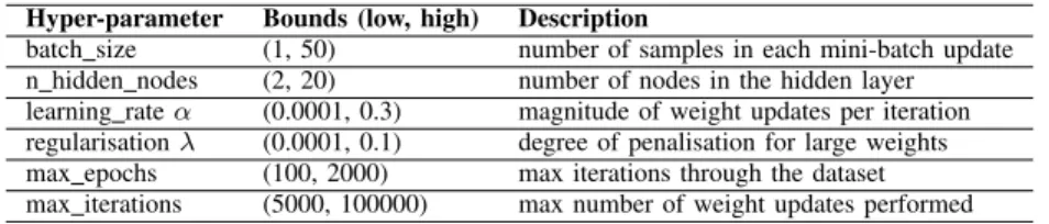
HYPERPARAMETERS ANDBOUNDS
Hyper-parameter Bounds (low, high) Description
batch size (1, 50) number of samples in each mini-batch update n hidden nodes (2, 20) number of nodes in the hidden layer learning rateα (0.0001, 0.3) magnitude of weight updates per iteration regularisationλ (0.0001, 0.1) degree of penalisation for large weights max epochs (100, 2000) max iterations through the dataset max iterations (5000, 100000) max number of weight updates performed
non (CW) and standardised (CW-sd) data.
Inputs: 14 features; weighted; outcome = classes; 6
binary and 5 continuous modifiable factors + age risk (4) and education risk (5c).
Each model was optimised on training set; those models with the best performance on the held-out validation data were selected as the best performing and as such had the optimum hyper-parameter configuration; finally the perfor-mance of those selected to have the optimal hyper-parameter configurations were evaluated on the further held-out test set, independent to the training and validation data. This ensures bias is not present in the model as it is not evaluated on the data it was trained on, mitigating against over-fitting and leading to better generalisation.
B. Model and Hyper-Parameter Optimisation Procedures As previously mentioned in Section II MSGD in conjunc-tion with early stopping was the model optimisaconjunc-tion pro-cedure for all models. Higher level termination parameters:
max_epochsandmax_iterationswhere the bounds can be seen in Table II were also in place if early stopping did not terminate the training. Hyper-parameters were optimised through random search consisting of 256 trials for each experiment. Random search has been shown to outperform grid-search [2] and the number of trials were chosen as per the guidelines also described in [2]. For each trial a configuration was drawn uniformly and randomly according to the bounds shown in Table II.
IV. EVALUATION ANDANALYSIS
All experiments were run on a Dell Optiplex 790 running 64-bit Windows 10 Home with an Intel Core i7-2600 quad-core 3.40 GHz CPU and 16.0GB of RAM. The code for the experiments was developed in Python using the Enthought Canopy (1.5.4.3105) distribution of 64-bit Python 2.7.9 and developed in PyCharm 4.5 IDE. The code makes use of NumPy 1.9.2, Theano 0.7.0 and their dependencies. The AUC and χ2 test of independence were calculated in JMP Version
11. The time taken to train a total of 3,584 models for un-standardised and un-standardised baseline, modifiable, modifiable with education and modifiable with age and education risk and continuous tests was 14.79 hours.
A. Evaluation Metrics
The evaluation measures used, where tp (true positives) are the sum of values predicted positive that are positive, tn (true
negatives) are the sum of values predicted negative that are negative are as follows:
• Precision. Thepositive predictive value which is a
pro-portion of values predicted positive that are actually positive: n predicted positivetp .
• Recall. The sensitivity/true positive rate (TPR) which is
the proportion of true positives to the actual number of positives in the dataset: n actual positivetp .
• True Negative Rate (TNR): Also calledspecificity, the
rate at which the classifier identifies actual negative cases: tn
n actual negative.
• F1 Score. This is a harmonic mean of precision and
recall: 2∗ precisionprecision+∗recallrecall.
• Accuracy. The proportion of correctly classified
in-stances: n predictionstp+tn .
• AUROC. Using varying thresholds, this function
evalu-ates True Positivevs False Positve trade-off.
• p> χ2. This chi-squared test is used to show that model predictions are significant where the rejection threshold isp > 0.05.
B. Results
In this section, we provide the results of our main research goal: the determination of those risk factors and their com-binations which best predict survival in the dementia study. Our evaluation will focus on our use of a series of statistical tests to determine the highest performing predictive models. We can only present the results of interactions found as in reality, these interactions can only be evaluated by our research collaborators, dementia specialists at the University of Maastricht and this work is currently in progress.
1) Survival Analysis Results: Our analysis focuses on the survivedclassification versus all other hazards, grouping pre-dictions ofdeath,dementiaandcensorship. Models performed well when classifyingsurvivalandcensorship, gave moderate results for death but poor results when predicting dementia. This negative performance is due to class imbalance, while having sufficient numbers of survival, death and censorship cases (roughly 400 censored samples) numbers for dementia (˜60) were too low.
Of the baseline experiments CB-sd performed best in the measures of F1, Accuracy, AUROC, and Significance with values of 0.6888, 0.6667, 0.7326 and 0.0002 respectively. CB performed best in the Precision and TNR measures with scores of 0.6296 and 0.7872 while B2 performed best for recall at
TABLE III
ANALYSISSUMMARYSTATISTICS
Summary Statistics for Survival Analysis
Precision Recall(TPR) TNR F1 Accuracy aAUROC b,cp> χ2
B2-sd 0.4727 0.8125 0.4423 0.5977 0.5833 0.6922 0.0187 CB 0.6296 0.4595 0.7872 0.53125 0.6429 0.7021 0.0024 CB-sd 0.6078 0.7949 0.5556 0.6888 0.6667 0.7326* 0.0002 BW1 0.6364 0.4118 0.84 0.5 0.6667 0.6921* 0.0221 BW1-sd 0.48 0.75 0.5 0.5854 0.5952 0.6797 0.0237 BW2-sd 0.6383 0.75 0.6136 0.6897 0.6786 0.7016* 0.003 BW3 0.5849 0.9118 0.56 0.7126 0.7024 0.7635 <0.0001 BW3-sd 0.4642 0.7429 0.3878 0.5714 0.5357 n/a 0.33 CW 0.4262 0.9286 0.375 0.5843 0.5595 0.7299 0.0043 CW-sd 0.5263 0.9091 0.4706 0.6667 0.6429 0.7693 0.0002
aCalculated by fitting logistic model (LM) between actual vs. predicted classifications. *LM parameter estimates unstable, due to low instance of a class in test set. bDegrees of freedom:3 in all but BW2-sd and BW3-sd, DOF: 6.
cFindings corroborated with LM as some instances ofχ2had cell counts<5.
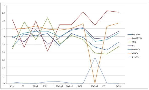
Fig. 1. Results
0.8125. For all experiments, BW2-sd had the highest Precision of 0.6383, CW had the highest Recall of 0.9286, BW1 had the best true negative rate of 0.84, BW3 had the highest F1, Accuracy and Significance at 0.7126, 0.7024 and < 0.0001 respectively. CW-sd had the highest AUROC of 0.7693. B1 and B1-sd, using only dementia diagnosis as outcome, pre-dicted every participant as ’not dementia’ and were therefore omitted, a result expected due to the previously described class imbalance. BW2 is also omitted from the results table due to poor performance. In summary, the performance of weighted experiments was superior to those of baseline experiments. It is important to note that the first 3 measures (Precision, Recall and TNR) are individual scores while the next 3 (F1,
Accuracy and AUROC) are different aggregations of these first 3 measures and as such, our working assumption is that the latter 3 measures carry more significance. Across the 3 aggregate measures, we feel that AUROC offers most significance as it provides the model with the best trade-off between true and false positives. This is followed by Accuracy as it delivers the model with the highest number of correct classifications.
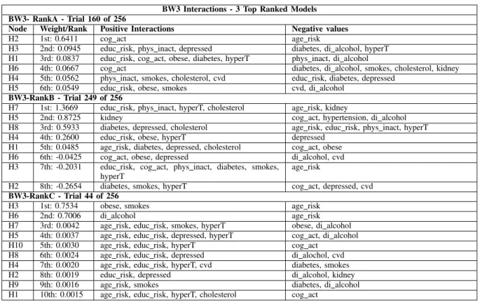
2) Risk Factor Interactions: It is from these high perform-ing models presented in Table III that we can extract the vari-able interactions illustrated in Tvari-able IV. These interactions are found from the top-3 runs of the BW3 experiment discussed in Section III-A and illustrate combinations of risks weighted
TABLE IV
TOPPERFORMINGRISKFACTORINTERACTIONS
BW3 Interactions - 3 Top Ranked Models BW3- RankA - Trial 160 of 256
Node Weight/Rank Positive Interactions Negative values
H2 1st: 0.6411 cog act age risk
H3 2nd: 0.0945 educ risk, phys inact, depressed diabetes, di alcohol, hyperT H1 3rd: 0.0837 educ risk, cog act, obese, diabetes, hyperT phys inact, di alcohol
H6 4th: 0.0667 cog act diabetes, di alcohol, smokes, cholesterol, kidney H4 5th: 0.0562 phys inact, smokes, cholesterol, cvd educ risk, diabetes, depressed
H5 6th: 0.0549 educ risk, obese, smokes cvd, di alcohol
BW3-RankB - Trial 249 of 256
H7 1st: 1.3669 educ risk, phys inact, hyperT, cholesterol age risk, kidney
H5 2nd: 0.8725 kidney cog act, hypertension, di alcohol H8 3rd: 0.5933 diabetes, depressed, cholesterol age risk, educ risk, phys inact, hyperT H4 4th: 0.2600 educ risk, obese, hyperT depressed
H1 5th: 0.0485 age risk, diabetes, depressed, cholesterol cog act, obese H6 6th: -0.0425 cog act, obese, depressed di alcohol, cvd H3 7th: -0.2031 educ risk, cog act, phys inact, diabetes, smokes,
hyperT
age risk
H2 8th: -0.2654 diabetes, smokes, hyperT cog act, depressed, cvd
BW3-RankC - Trial 44 of 256
H3 1st: 0.7534 obese, smokes age risk H6 2nd: 0.7006 di alcohol age risk H7 3rd: 0.0042 age risk, educ risk, smokes, hyperT obese, di alcohol H5 4th: 0.0037 age risk, educ risk, depressed, hyperT cog act, di alcohol H10 5th: 0.0030 age risk, educ risk, hyperT cog act
H8 6th: 0.0024 age risk, educ risk, depressed di alochol, cvd H4 7th: 0.0020 age risk, educ risk, hyperT, cvd diabetes, smokes H2 8th: 0.0019 educ risk, depressed di alcohol, kidney H9 9th: 0.0016 age risk, smokes diabetes, di alcohol H1 10th: 0.0015 age risk, educ risk, hyperT, cholesterol cog act
above average for the negative and positive weights for each node, as shown in Table IV. Put simply, the top interaction was that which occurred most often: cvd (cardiovascular disease) and di alcohol, occurring in all three models. Other interactions like diabetes and smokes occur often together but also in the context of other variables so need further validation. For the remainder of this section, we focus on the discussion and analysis of the approach and results which delivered these interactions, as clusters of Risk Interactions can only be evaluated by clinical researchers.
C. Discussion and Analysis
BW3-sd aside, all models were found to be significant under a chi-squared test of independence. Significance of BW3 performed poorly at 0.33 meaning predictions achieved could be due to chance. We conclude poor performance of BW3-sd is likely due to the standardisation process. Weighted features had continuous values, but further analysis shows they are technically ordinal - either 0 or the risk weight - hence, do not follow a normal distribution. Feature scaling (subtracting the min value and dividing by the range) instead of standardising (subtracting the mean and dividing by the standard deviation) would provide greater benefit in this context and will be explored in future work. As a result, all BW models apart from BW2 performed better when unstandardised, in contrast to continuous models which performed better when standardised. The opposite effect found for BW2 is likely due to the continuousagewhich is on a much wider scale than the other
features and thus, we conclude that standardising the dataset improved performance.
Models built from continuous data performed better than those only including binary features, where binary features pertain to the participant either having or not having a risk factor. Weighted models also performed better than their non-weighted counterparts. Binary models only begin to outper-form the continuous baseline wheneducationrisk is added in BW2. Continuous data provides far more information than bi-nary with the result that CB outperforms BW1 untileducation andage/sexrisks (significant predictors of dementia) are added in BW2 and BW3 respectively. The negative performance B2 shows risk weightings have a significant role to play in survival analysis in the absence of continuous data. BW2 performs better than BW1 and likewise BW3 performs better than BW2, with increasing AUROC for each. Further information is given to each model, first incorporatingeducationrisk and subsequently then incorporatingage/sexrisk. The key conclu-sion here is that continuous data and relative risks improve the predictive accuracy of the model. This is important, as currently the In-MINDD model developed by the clinicians only contains dichotomous has/does not have variables for each particular risk factor.
When considering the aggregate measures, BW3 performs best with highest F1, Accuracy and Significance, the only model with F1 and Accuracy > 0.7. Therefore, BW3 was the most accurate classifier, correctly classifying the highest number of instances (Accuracy) and performing best at
identi-fying and predicting positive instances (F1). The significance (p > χ2) of < 0.0001 shows that BW3 achieved predictions
that are the most significant and the least likely to be due to chance. CW-sd achieved the best AUROC score of 0.7693 and a close to best significance level of 0.0002. Thus, we observe that CW-sd had the greatest trade-off between true and false positives, a very important factor in survival analysis. Also CW-sd predictions are veryunlikely due to chance (0.0002). The difference in AUROC for BW3 and CW-sd is very small at 0.0058 or 0.58%. BW3’s greater performance is likely due to relative risk weights being designed for dichotomous risk factor cut-offs rather than continuous scores. On the other hand, continuous data was present for only 5 out of 11 risk factors in the dataset and if continuous measures were used for all features then continuous models would likely surpass binary models on all scores.
CW has the highest TPR of 0.9286, meaning out of the instances it predicted positive,>92% wereactuallypositive -an excellent score - but offset by poor Precision of < 0.5, worse than the binary baseline. Using the positive values in the test set, it identified <50% which is reflected in its poor F1 score of 0.5843 and lower level of significance. We conclude this is likely due to lack of standardisation. BW1 has highest true negative rate at 0.84, but has a poor TPR of < 0.5. Although performing better than other models in predicting hazards (negative cases), the low TPR shows us this model could not perform well in modelling survival cases. This is undesirable as <50% of those it predicted positive, were actually positive, with many of these as false positives.
In summary, the important conclusion from the results is that even when the relevant risk weights are omitted and only dichotomous values are present, the model is still significantly predicting survival, showing that these particular factors are valid in the prediction of survival versus other hazards. Fur-thermore, models which include relative risk weights from the literature experience an improvement in predictive accuracy. Our results show that continuous data can again improve the model. Although the final binary model outperforms the continuous model in some measures, as continuous data is only present for 5 of the 11 inputs we are confident that when continuous measures are added for all inputs that it will out-perform all binary models. With respect to input interactions we have successfully presented those automatically learned by the MLP.
V. RELATEDRESEARCH
Although there is potential for artificial neural networks (ANN) in survival analysis, it is not in widespread use for clinical applications. Neural networks in the context of health analytics have been shown to be at worst, on par with tradi-tional regression approaches [16], [10] and at best outperform these methods [20]. Health benefits accrued from using ANNs in medical interventions have been shown to have significant impact in their application, where notable examples include cervical cytology and the early detection of acute myocardial infarction (heart attack) [9]. Therefore, the motivation for
the application of these methods to the field of dementia is significant.
The majority of ANN survival analyses focus on post-surgery patient mortality or relapse, in areas such as pancreatic cancer [1], breast cancer [10] and liver cancer [20]. ANNs have been applied to dementia, [11], [12], but as far as we can identify from the literature, none adopt a survival analysis paradigm with respect to dementia as explored in this work. Furthermore, all discussed research compares ANNs to methods such as Cox’s regression or non-neural machine learning algorithms. This research evaluates ANNs built on modifiable risk factors with those including non-modifiable factors. We add to the research through the comparison of non-modifiable and modifiable risk factor models for dementia and by using a survival analysis paradigm. Finally, none of the aforementioned works analyse latent features learned in the hidden layers to extract input features interactions, which are clinically relevant, as these model risk factor interactions and increase a classifier’s predictive power. This insight could provide further understanding to clinicians as to why ANNs would better model survival and can perhaps identify novel interactions from the data which might not be attainable from traditional means. Variable interactions learned during an ANN survival analysis are analysed in [5], but again this in the context of surgery survival and not dementia, which is a further focus of this work.
Exploring [11] further, two (MLP and radial basis function) neural nets are found to perform worse than Support Vector Machines (highest), Random Forests and Linear Discriminant Analyses. ANNs are complex to train, so there are several likely reasons for poor performance, as discussed by the authors. Primarily, ANNs are highly sensitive to tuning (hyper) parameters used to initialise and inform the training proce-dure, vastly effecting model quality. [11] only optimise the number of hidden nodes, where all other settings were those ”commonly used in data mining applications” i.e. not fitted to the data. Furthermore, [11] use a grid-search optimisa-tion procedure, in contrast to random search for all hyper-parameters - employed by this research - a methodology shown to outperform grid-search [2]. Finally, their cross-validation approach is sub-optimal for hyper-parameters evaluation and choice. Their strategy essentially splits the data in two - a portion for training and evaluating hyper-parameters and a held-out cross-validation set for evaluating the classifier’s final performance. When data on which the model is trained is also used to evaluate hyper-parameter performance, this effectively over-fits the hyper-parameters to the training data. Instead, a three-way split is advised, building the model on training data, evaluating hyper-parameters on held-out cross validation data and an independent test set to evaluate classifier performance on completely unseen data. The latter approach adopted in this work, as well as an automated random search method for hyper-parameter optimisation which has been shown to improve a classifier’s predictive power [2]. Furthermore, [11] do not apply ANNs in the context of dementia survival, but instead for dementia classification and none of the latent
features learned by the network were analysed.
In [13], the authors model latent classes (behaviours) in dementia analysis, showing the approaches relevance and according to the authors, the sole study to do so for dementia. The analysis attempts to determine sub-behaviours across six domains: church-attendance; smoking; alcohol use; social interaction; and physical exercise. LCA requires a number of further steps after the identification of classes. First, LCA is applied and tested for a variety of possible latent class numbers (similar to our number of nodes), then multi-nominal regres-sion is applied to assign a sample to the relevant class (be-havioural sub-category) before finally running regression again (for each identified class) to evaluate survival probabilities. In our work we use an MLP to automate this process of learning latent variables. An MLP essentially aggregates all steps and where latent variables are identified, samples activate relevant latent variables (hidden nodes) and classification probabilities are identified, all during the course of training. In addition we have extracted non-linear continuous interactions between sub-categories with the MLP in contrast to the linear LCA, thus providing more representative abstract classes.
VI. CONCLUSIONS ANDFUTUREWORK
Dementia is a major health concern with the projected numbers likely to consume countries’ health budgets in years to come. While many specialists in this field together with clinical researchers are involved in longitudinal studies in an effort to determine the prominent interactions between risk factors, this is a difficult task, given the numbers of risk factors, the permutations possible, and the application of weightings to each risk factor. While the In-MINDD project connects clinical researchers to trial participants through a cloud-based profiler, it is only by connecting the third stakeholder, the data scientist, that we can deliver greater impact.
In this research, we describe our neural network service which using a series of validation functions, supports the profiler by determining the set of interacting risk factors in the highest performing prediction models with varying degrees of modifiable and non-modifiable risk-factors. As part of our evaluation, we present the results of experiments for 10 predic-tive models, each of which had 512 test configurations across 7 parameters to determine the highest performing model. Our goal was two-fold, first build a non-linear predictive model of dementia survival with a Multi-Layer Perceptron and second examine its hidden features to establish clusters of risk factors which we could then provide to clinical research colleagues for evaluation. This builds on existing research as although ANNs have been applied in a survival analysis paradigm before - as far as we are aware - they have not been applied to dementia survival analysis. Furthermore, in the dementia context the hidden layers have not been analysed to extract candidate clusters of risk factors, which has been presented in this work. Finally, this work adds a procedure which automates the optimisation and selection of the MLP’s hyper-parameters using random search in contrast to previous works which often did not optimise all hyper-parameters, or did so in a
manual grid-search fashion. The result of this is a predictive model which significantly predicts dementia survival and sets of candidate risk factor interaction which we will provide to dementia experts who can evaluate these from a clinical stand-point.
ACKNOWLEDGEMENT
Research funded by In-MINDD, an EU FP7 project, Grant Agreement Number 304979 and Science Foundation Ireland under grant number SFI/12/RC/2289.
We would also like to acknowledge the In-MINDD team, specifically Martin Van Boxtel, Sebastian K¨ohler and Kay Deckers at Maastricht University for the provision and ex-planation of their work and data.
REFERENCES
[1] Ansari, D., Nilsson, J., Andersson, R., Regn´er, S., Tingstedt, B., An-dersson, B.: Artificial neural networks predict survival from pancreatic cancer after radical surgery. The American Journal of Surgery 205(1), 1–7 (2013)
[2] Bergstra, J., Bengio, Y.: Random search for hyper-parameter optimiza-tion. J. Mach. Learn. Res. 13, 281–305 (Feb 2012)
[3] van Boxtel, M.P., Buntinx, F., Houx, P.J., Metsemakers, J.F., Knottnerus, A., Jolles, J.: The relation between morbidity and cognitive performance in a normal aging population. The Journals of Gerontology Series A: Biological Sciences and Medical Sciences 53(2), M147–M154 (1998) [4] Consortium, I.M.: In-mindd website (2014), www.inmindd.eu, online;
Last accessed 31/01/14; www.inmindd.eu
[5] De Laurentiis, M., Ravdin, P.: Survival analysis of censored data: Neural network analysis detection of complex interactions between variables. Breast Cancer Research and Treatment 32(1), 113–118 (1994) [6] Deckers, K., Boxtel, M.P., Schiepers, O.J., Vugt, M., Mu˜noz S´anchez,
J.L., Anstey, K.J., Brayne, C., Dartigues, J.F., Engedal, K., Kivipelto, M., et al.: Target risk factors for dementia prevention: a systematic review and delphi consensus study on the evidence from observational studies. International journal of geriatric psychiatry (2014)
[7] Europe, A.: The prevalence of dementia in europe, online; http://www.alzheimer-europe.org/Policy-in-Practice2/Country-comparisons/The-prevalence-of-dementia-in-Europe; Last Accessed 22/11/2015
[8] International, A.D.: Dementia statistics uk. 2014, online; Last accessed 22/11/2015; http://www.alz.co.uk/research/statistics
[9] Lisboa, P.J.: A review of evidence of health benefit from artificial neural networks in medical intervention. Neural networks 15(1), 11–39 (2002) [10] Lisboa, P., Wong, H., Vellido, A., Kirby, S., Harris, P., Swindeil, R.: Survival of breast cancer patients following surgery: a detailed assess-ment of the multi-layer perceptron and cox’s proportional hazard model. In: Neural Networks Proceedings, 1998. The 1998 IEEE International Joint Conference on. vol. 1, pp. 112–116 vol.1 (May 1998)
[11] Maroco, J., Silva, D., Rodrigues, A., Guerreiro, M., Santana, I., de Mendonc¸a, A.: Data mining methods in the prediction of dementia: A real-data comparison of the accuracy, sensitivity and specificity of linear discriminant analysis, logistic regression, neural networks, support vector machines, classification trees and random forests. BMC research notes 4(1), 299 (2011)
[12] Maroco, J., Silva, D., Guerreiro, M., de Mendona, A., Santana, I.: Pre-diction of dementia patients: A comparative approach using parametric versus nonparametric classifiers. In: Advances in Regression, Survival Analysis, Extreme Values, Markov Processes and Other Statistical Applications, pp. 269–280. Studies in Theoretical and Applied Statistics, Springer Berlin Heidelberg (2013)
[13] Norton, M.C., Dew, J., Smith, H., Fauth, E., Piercy, K.W., Breitner, J., Tschanz, J., Wengreen, H., Welsh-Bohmer, K.: Lifestyle behavior pattern is associated with different levels of risk for incident dementia and alzheimer’s disease: the cache county study. Journal of the American Geriatrics Society 60(3), 405–412 (2012)
[14] O Donnell, C.A., Browne, S., Pierce, M., McConnachie, A., Deckers, K., van Boxtel, M.P., Manera, V., K¨ohler, S., Redmond, M., Verhey, F.R., et al.: Reducing dementia risk by targeting modifiable risk factors in mid-life: study protocol for the innovative midlife intervention for dementia deterrence (in-mindd) randomised controlled feasibility trial. Pilot and Feasibility Studies 1(1), 1 (2015)
[15] O’Donoghue, J., Roantree, M.: A framework for selecting deep learning hyper-parameters. In: Maneth, S. (ed.) Data Science - 30th British International Conference on Databases, BICOD 2015, Edinburgh, UK, July 6-8, 2015, Proceedings, Lecture Notes in Computer Science, vol. 9147, pp. 120–132. Springer International Publishing (2015)
[16] O’Donoghue, J., Roantree, M., Boxtel, M.V.: A configurable deep network for high-dimensional clinical trial data. In: Neural Networks (IJCNN), 2014 International Joint Conference on. IEEE (July 2015) [17] Roantree, M., McCann, D., Moyna, N.: Integrating sensor streams
in phealth networks. In: Parallel and Distributed Systems, 2008. IC-PADS’08. 14th IEEE International Conference on. pp. 320–327. IEEE (2008)
[18] Roantree, M., ODonoghue, J., OKelly, N., Boxtel, M.v., Kohler, S.: Automating the integration of clinical studies into medical ontologies. In: System Sciences (HICSS), 2014 47th Hawaii International Conference on. pp. 2938–2947. IEEE (2014)
[19] Roantree, M., ODonoghue, J., OKelly, N., Pierce, M., Irving, K., Van Boxtel, M., K¨ohler, S.: Mapping longitudinal studies to risk factors in an ontology for dementia. Health Informatics Jour-nal pp. 1–13 (2015), http://jhi.sagepub.com/content/early/2015/01/04/ 1460458214564092.long
[20] Shi, H.Y., Lee, K.T., Lee, H.H., Ho, W.H., Sun, D.P., Wang, J.J., Chiu, C.C.: Comparison of artificial neural network and logistic regression models for predicting in-hospital mortality after primary liver cancer surgery. Plos One 7 (2012)
[21] Yang, Q., Wu, X.: 10 challenging problems in data mining research. International Journal of Information Technology and Decision Making 5(4), 597–604 (2006)