Comparison of Particle Methods : SPH and MPS
Sunao Tokura
Tokura Simulation Research Corporation
Abstract
SPH (Smoothed Particle Hydrodynamics) implemented in LS-DYNA® has been used widely in various industrial fields as a reliable and robust particle method. At present SPH is considered as one of major numerical simulation method for compressible fluid and solid materials.
Recently a unique particle method called MPS (Moving Particle Simulation) has been developed and started to use for some industrial application as a CFD (Computational Fluid Dynamics) solver for incompressible flow. As most application for fluid flow in industry are incompressible, MPS may have a potential ability to treat such problems efficiently than SPH. Both methods have common characteristics that particles are used to discretize continuum domain to be solved. However, as the numerical procedures to solve the governing equation are very different, each numerical simulation method has both inherent advantages and disadvantages. This paper demonstrates the comparison of SPH and MPS for some engineering problems and intends to reveal the difference of these two methods. Comparison of numerical simulation techniques should be very useful for further understanding about multiphysics capability of LS-DYNA even for expert LS-DYNA users. Surface tension model, turbulence model, treatment of Newtonian and Non-Newtonian fluid, coupling with structures and other several topics are discussed. In addition an FSI (Fluid Structure Interaction) problem using MPS software and LS-DYNA is demonstrated in the presentation. In this FSI problem a vehicle is washed away by a tsunami and crashes against a rigid wall. Pressure of tsunami on the surface of the vehicle is computed by MPS software and the deformation of the auto body is calculated by LS-DYNA.
Introduction
SPH in LS-DYNA® is very useful capability to model fluids. However it may not be suitable for incompressible or nearly incompressible fluids as SPH is formulated for compressible fluid dynamics. Meanwhile another particle method for incompressible fluid dynamics called MPS has been developed[1]. Formerly MPS was the abbreviation of Moving Particle Semi-implicit
method, but currently Moving Particle Simulation method as fully explicit version of the solver has also been developed. One of major difference of compressible and incompressible fluid solvers is time step size. For example time step sizes of SPH in LS-DYNA and MPS are given as follows; compressible (1) incompressible (2) max 0 u l t c l t MPS SPH
where, ; Courant number, l ; characteristic length, l0 ; the distance of particles, c ; sound speed and umax ; maximum flow velocity. Generally since c >> umax, tMPS is typically 100 to 1000 times larger than tSPH. So MPS has potential ability to solve incompressible flow problem very efficiently. In addition MPS has many features required to treat CFD problem accurately. At present a CFD software "Particleworks" has been developed based on MPS method[2]. In this presentation major differences between SPH and MPS are shown. Although Particleworks has a capability to compute FSI problem, structures can be treated as only rigid body. So weak (one-way) coupling procedure to estimate the damage of structure using Particleworks and LS-DYNA is also demonstrated.
MPS Method Outline
The governing equations for incompressible flow are the continuity and the Navier-Stokes equations,
(3)
(4)
where, ; density, u ; velocity, P ; pressure, ; diffusion coefficient, and g ; gravity. MPS defines the kernel function as,
(5)
Fig.1 MPS kernel function
A particle interacts only with surrounding particles within the radius re. Particle number density is defined using the kernel function,
(6)
Mathematical operations acting on arbitrary scalar and vector u at particle i are defined as the particle interaction approximation model as follows:
g u u 2 1 0 P Dt D Dt D ) ( 0 ) ( 1 ) ( e e e r r r r r r r w
i j i j i w n r rwhere, d ; spatial dimension (2 or 3), n0 ; initial particle number density, and ; correction coefficient. The governing equation Eq.4 is discretized using Eq,7 and solved under the condition Eq.3 with a semi-implicit algorithm similar to the conventional Simplified MAC method. On the other hand SPH has the kernel function as follows,
(8)
Fig.2 Kernel functions
We need the discritization form of gradP to solve the governing equation. In SPH formulation spatial distribution of P is approximated first. And gradP is defined as follows,
(9)
(10)
where, mi and i are mass and density of particle i respectively. In the MPS procedure gradP is obtained from Eq.7a directly,
i j i j i j i i j i j i j i j ij i i j i j i j i j i j i j i w n d w u n d w n d r r r r r r r r u r r r r r r r r 0 2 2 0 0 2 2 gradient model (7a)
divergence model (7b) Laplacian model (7c)
u
for
u
for
u
u
for
u
u
u
h
C
h
u
w
2
0
2
1
2
4
1
1
0
4
3
2
3
1
,
3 3 2 -xr 0 xr -xr 0 xr MPS SPH
N j j i i j j j i N j j i j j h x x w x P x P m x P h x x w x P m x P 1 1 , , (11)
Equation 10 involves gradient of w, while Eq.11 does not. This means that MPS can adopt non differentiable kernel function (Fig.2). The form of Eq.5 can prevent duplication of particles and it contributes to numerical stability.
Modeling of Influence of Wall
Since MPS is incompressible, influence of the wall to the particle near the wall should be included in the interaction model Eq.7, i.e., pressure gradient caused by the wall for particle i is defined as follows,
(12)
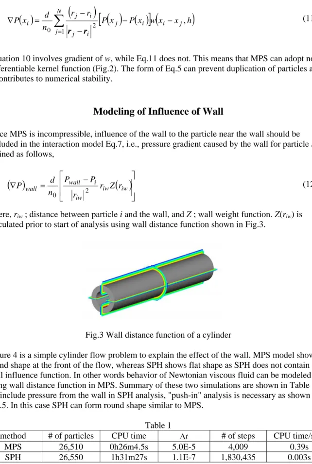
where, riw ; distance between particle i and the wall, and Z ; wall weight function. Z(riw) is calculated prior to start of analysis using wall distance function shown in Fig.3.
Fig.3 Wall distance function of a cylinder
Figure 4 is a simple cylinder flow problem to explain the effect of the wall. MPS model shows round shape at the front of the flow, whereas SPH shows flat shape as SPH does not contain any wall influence function. In other words behavior of Newtonian viscous fluid can be modeled using wall distance function in MPS. Summary of these two simulations are shown in Table 1. To include pressure from the wall in SPH analysis, "push-in" analysis is necessary as shown in Fig.5. In this case SPH can form round shape similar to MPS.
Table 1
method # of particles CPU time t # of steps CPU time/step
MPS 26,510 0h26m4.5s 5.0E-5 4,009 0.39s SPH 26,550 1h31m27s 1.1E-7 1,830,435 0.003s
N j j i i j i j i j i P x P x w x x h r r n d x P 1 2 0 , r r
iw iw iw i wall wall r Z r r P P n d P 2 0Fig.4 Cylinder flow problem with constant inflow velocity
Fig.5 "push-in" analysis to simulate Newtonian viscous flow in SPH
Surface Tension
Surface tension is considered in Particleworks using Continuum Surface Force (CSF) model. CSF is commonly used technique in many conventional mesh based CFD codes. The governing equation including surface tension term can be written as,
(12)
where, ; constant, ; curvature, ; delta function to limit force acting on the surface particle only, and n ; normal vector of surface. CSF model adds surface tension force proportional to curvature on the particle on the free surface. MPS calculates curvature using particle number densities as follows,
(13)
where, re; influence radius, n0st ; particle number density of flat surface, and nist ; particle number density of convex surface. CSF model image in MPS is shown in Fig6. If nist = n0st, curvature becomes to zero. n g u u 1 1 2 P Dt D st st i e n n r 0 2 , cos 2 MPS model SPH model
Fig.6 Surface tension model in MPS
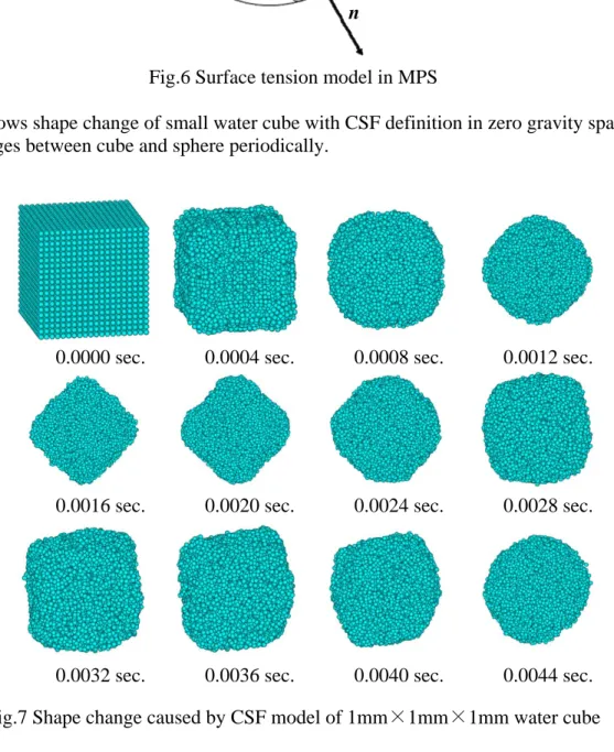
Figure 7 shows shape change of small water cube with CSF definition in zero gravity space. The shape changes between cube and sphere periodically.
Fig.7 Shape change caused by CSF model of 1mm×1mm×1mm water cube Figure 8 is a water splay on a flat plate using SPH and MPS. Aggregation of particles can be seen in MPS case because of surface tension effect, whereas particles scatter on the surface in SPH case. If behavior of water on windshield or auto body is simulated, surface tension model may be necessary to get realistic results.
re
n
0.0032 sec. 0.0036 sec. 0.0040 sec. 0.0044 sec. 0.0016 sec. 0.0020 sec. 0.0024 sec. 0.0028 sec. 0.0000 sec. 0.0004 sec. 0.0008 sec. 0.0012 sec.
Fig.8 Water splay on flat plate
Turbulence Model
Turbulence model is required to consider the effect of chaotic local flow smaller than model resolution. LES (Large-eddy simulation) is one of standard numerical procedure to treat turbulence in CFD community and is implemented in Particleworks. Turbulence effect may influence global flow behavior in some application. Gear oil flow problem was solved to
investigate the effect of turbulence model. Figure 9 shows the results of the analyses using MPS with and without LES. Particleworks has a capability to count the number of particles in
specified region. So a box region was defined in front of the gear and the change of the number of particles in the box was compared for two cases as shown in Fig.10. Clearly the case with LES moves up more oil than the case without LES. As SPH in LS-DYNA has no turbulence model, similar analysis may estimate the quantity of moved-up oil fewer than real.
(a) LES off (b) LES on Fig.9 Gear oil flow simulation using MPS
0.1 sec. 0.2 sec. 0.3 sec. MPS
Fig.10 Number of particles history
Application Example using MPS and LS-DYNA
Particleworks can compute FSI problem. But structures that interact with fluid are treated as only rigid body. FSI using LS-DYNA is also possible but very time consuming. Combination of MPS and LS-DYNA may be a practical solution to model FSI problem. One of the application
example using MPS and LS-DYNA is a tsunami simulation of vehicles. The damage of the vehicle drifted by tsunami should be estimated. If passengers can move out from the drifted vehicle opening the door, many people may survive from the disaster. Safer design to protect passengers from tsunami may be possible. In this scenario, procedure of simulation is considered as follows;
(1) Perform tsunami simulation using MPS. In this simulation vehicle is modeled as a rigid body using STL format geometry. Vehicle is constructed using rigid body particle cluster
generated in given STL geometry as shown in Fig.11. The vehicle is washed away and impacts with a rigid wall.
(2) Pressure history of the vehicle is obtained from MPS simulation. Pressure is calculated on each rigid particle and it is mapped on the STL vertexes.
(3) Pressure at the particles on the surface of the vehicle is converted as pressure history load data acting on each finite element. The particle closest from a shell element is searched. (4) Execute crash simulation of the vehicle against the rigid wall. The vehicle is pushed toward
the rigid wall by the pressure load.
In the MPS tsunami simulation, the flow of the tsunami and the behavior of the vehicle are obtained as shown in Fig.12. A vehicle is placed at the position of 1,000 mm from a rigid wall at the beginning of the simulation. Water comes in the model from the inflow with the velocity 4,000 mm/s. The vehicle are washed away and crashes into the wall.
Box definition to count the number of particles
The event interval was 1.35 seconds. In this simulation pressure history acting on the surface of the vehicle was obtained. The pressure was calculated on each particle during the simulation and then it was mapped on the STL vertexes by post processing. After the tsunami simulation, pressure history was converted into pressure load for LS-DYNA crash simulation. In the
mapping process the pressure at the closest rigid particle to a shell element center was applied on the element surface as a pressure load. Figure 13 shows the mapping process of pressure
distribution through particles to finite elements. In the second stage, transient analysis of the vehicle model[4] using LS-DYNA was executed. Through the simulation, deformation and stress distribution was obtained. Figure 14 shows the deformed geometry and Mises stress distribution of the vehicle. Large deformation can be seen not only in the right hand side of the vehicle where the vehicle contacts with the rigid wall, but also in the left hand side.
Fig.11 STL vehicle geometry and generated rigid particle of vehicle for MPS simulation
t=0.05 sec. 0.5 sec. 0.75 sec. 0.95 sec. Fig.12 Result of tsunami simulation using MPS
inflow
Particles STL vertexes FEM shell elements Fig.13 Example of mapping result of pressure distribution at time = 0.85 sec. 0 10
Conclusions
One of particle method MPS for incompressible flow was introduced and compared with SPH for compressible flow. These examples showed that MPS had practical capabilities, i.e., surface tension model and turbulence model and so on. In addition one way coupling procedure using MPS and L-DYNA for FSI problem was also explained in the paper.
References
[1] S. Koshizuka and Y. Oka: Moving-Particle Semi-Implicit Method for Fragmentation of Incompressible Fluid, Nuclear Science and Engineering, Vol.123, pp.421-434, 1996. [2] http://www.prometech.co.jp/
[3] Sunao Tokura and Takumi Kasahara, Simulation Technique to Estimate Damages of Auto Body Washed Away by Flooding, COMPSAFE 2014
[4] FHWA/NHTSA National Crash Analysis Center, http://www.ncac.gwu.edu/ right view (wall side) left view (tsunami side)
Fig.14 Deformation and Mises stress distribution of the vehicle at 1.0 second. 200 Mises stress (MPa)
100