c
EXPLORING MODEL PARALLELISM IN DISTRIBUTED SCHEDULING OF NEURAL NETWORK FRAMEWORKS
BY
PALLAVI SRIVASTAVA
THESIS
Submitted in partial fulfillment of the requirements for the degree of Master of Science in Computer Science
in the Graduate College of the
University of Illinois at Urbana-Champaign, 2018
Urbana, Illinois Adviser:
ABSTRACT
The growth in size and computational requirements in training Neural Networks (NN) over the past few years has led to an increase in their sizes. In many cases, the networks can grow so large that can no longer fit on a single machine. A model parallel approach, backed by partitioning of Neural Networks and placement of operators on devices in a distributed system, provides a better distributed solution to this problem. In this thesis, we motivate the case for device placement in Neural Networks. We propose, analyze and evaluate m-SCT, a polynomial time algorithmic solution to this end. Additionally, we formulate an exponential time optimal ILP solution that models the placement problem. We summarize our contributions as:
1. We propose a theoretical solution to the memory constrained placement problem with makespan and approximation ratio guarantees.
2. We compare and contrast m-SCT with other state of the art scheduling algorithms in a simulation environment and show that it consistently performs well on real world graphs across a variety of network bandwidths and memory constraints.
3. We lay the foundation for the experimental evaluation of the proposed solutions in existing Machine Learning frameworks.
ACKNOWLEDGMENTS
I would like to thank my advisor, Professor Indranil Gupta, for his continual support and advice. I would also like to thank my colleagues and collaborators, Linda Cai and Jintao Jiang, without whom this thesis could not have been written.
TABLE OF CONTENTS
LIST OF ABBREVIATIONS . . . vii
CHAPTER 1 INTRODUCTION . . . 1
1.1 Contribution of this Thesis . . . 2
1.2 Outline of this Thesis . . . 3
CHAPTER 2 PRELIMINARIES . . . 5
2.1 Systems Preliminaries . . . 5
2.2 Algorithm Preliminaries . . . 7
CHAPTER 3 PROBLEM STATEMENT, MOTIVATION, AND PRIOR WORK . . 8
3.1 Problem Statement . . . 8
3.2 Motivation . . . 8
3.3 Prior Work . . . 9
CHAPTER 4 ALGORITHM DESIGN . . . 12
4.1 Topological Sort . . . 12
4.2 ETF . . . 13
4.3 SCT . . . 13
4.4 Optimal Solution . . . 17
CHAPTER 5 BACK PROPAGATION . . . 22
5.1 Definition and Need for Back Propagation . . . 22
5.2 Accounting for Back Propagation . . . 22
5.3 Scheduling Strategy . . . 22
5.4 Guarantees . . . 23
CHAPTER 6 IMPLEMENTATION . . . 27
6.1 Simulation . . . 27
6.2 Estimation of Computation time . . . 27
6.3 Estimation of Communication time . . . 28
6.4 Constraints . . . 29
6.5 Linear Programming Solver . . . 30
CHAPTER 7 EXPERIMENTAL RESULTS . . . 31
7.1 Fixed Total Memory Experiments . . . 31
7.2 Variable Total Memory Experiments . . . 35
CHAPTER 8 REFLECTION . . . 39
8.1 Approximation of the ILP Solution . . . 39
8.2 Future Directions . . . 41
CHAPTER 9 CONCLUSION . . . 42
CHAPTER 10 FUTURE WORK . . . 44
LIST OF ABBREVIATIONS
NN Neural Network
TF TensorFlow
LP Linear Programming
ILP Integer Linear Programming CNN Convolution Neural Network SCT Small Communication Time
UET-UCT Unit Computation Time Unit Communication Time ETF Earliest Task First
RNN Recurrent Neural Network LSTM Long Short-Term Memory FFN Feed Forward Neural Network NMT Neural Machine Translation
CHAPTER 1: INTRODUCTION
The past few years have seen a huge shift in interest towards Machine Learning. With the advent of deep learning, the complexity in training Neural Networks (NN) has increased manifold. The training process is expensive, resource intensive and time consuming. The time increases as the models become more complex and training data increases. For instance, in [1], training the 152-layer neural network for one iteration requires 11.3 billion floating point operations and the model is trained up to 6×10⁵ iterations.
In order to keep up with the infrastructure requirements of such explosive growth, dis-tributed computing in Machine Learning is the focus of a lot of current research [2] [3] [4] [5] and software development.
The software industry has universalized the usage of many specialized NN frameworks that are not only optimized to shorten the training time, but also standardize the development of Machine Learning algorithms. Several of these frameworks such as MXNet [4], Torch7 [6], Theano [7] and TensorFlow [8] are described in more detail in chapter 2.
Recent research has led to multiple developments in data parallelism [9] [10] [11]; a tech-nique which focuses on distributing data across different processors, each possessing an independent copy of the model. This approach stems from SIMD (single instruction, mul-tiple data) computer architecture [12, p. 182], one of the oldest ways of parallel processing on computers. Adequate user support has been provided for these techniques in leading Machine Learning (ML) frameworks [4] [6] [13] [7] [14] such as TensorFlow (TF) [8] [15]. While data parallelism is an effective way to handle burgeoning training data, it does little to alleviate the problems caused by the ever increasing size of the models themselves as they become more complex.
Model parallelism is an effective way to handle this issue as it distributes a single model across multiple processors which independently compute model parameters for the part of the model assigned to them. In parallel computing terms, it can be thought of as MPSD (multiple program, single data). Model parallelism can prove to be an indispensable tool for NN models which are too big to fit on a single machine. However, there is no explicit support for users to deploy this technique on most ML engines effectively and users are required to manually place parts of the model on different processors in an arbitrary fashion. Recent work on optimization of these placements [16] make use of reinforcement learning and are a step up from human expert placements and heuristics. However, using reinforcement learning
explore multiple models such as k-min cut and scheduling with communication delay to fit the problem. Our aim is to provide a relatively fast, easy to deploy and effective theoretical solution for this problem.
1.1 CONTRIBUTION OF THIS THESIS
1. We introduce the concept of wait time and use it to establish why scheduling with communication delay is preferred over k-min cut to model the placement problem. 2. In chapter 2 (section 4.4), we formulate an integer linear programming (ILP) problem
using the placement problem constraints (including memory constraints). The running time for this optimal solution isO(2n2), where n is the total number of nodes.
3. In chapter 8, we further demonstrate the difficulty in applying LP relaxation or other convex optimization relaxation techniques to approximate the optimal solution in poly-nomial time.
4. Next, in chapter 4 (section 4.3.2), we propose m-SCT, a modified version of the SCT algorithm [17] that incorporates memory constraints in the system. We prove the modified approximation ratio to be within (1+(2+2+2ρ)ρm)· 1
K−1 of the finite SCT algorithm
approximation ratio, where the total memory available on all machines isK times the total memory required by the network, m is the number of available machines, and ρ is ratio between the maximum communication time between any two nodes and the minimum computation time for any node.
5. Both the optimal formulation and the m-SCT algorithm expect a directed acyclic graph (DAG). Since back-propagation in neural networks introduces some cycles, in chapter 5, we first establish the makespan for the forward computation case and put forth a mathematical proof (section 5.4.2, theorem 5.3) showing that the approximation ratio remains unchanged after back-propagation. Furthermore, we show that the makespan of the backward pass is within C0 times the makespan for the forward pass (section
5.4.2, theorem 5.1), where C0 is the maximum ratio between (a) corresponding
back-ward pass edge weight and forback-ward pass edge weight and (b) corresponding backback-ward pass node weight and forward pass node weight.
6. In chapter 7, we experimentally compare the performance of SCT, ETF and m-TOPO using simulation. We vary the bandwidth and the total number of processors for
all experiments. For each case, we experiment under two memory constraints (a) fixed total memory in the system (section 7.1) and (b) fixed amount of memory available on each machine (section 7.2). We show that m-SCT consistently performs well for large bandwidth for both Inception-V3 and our small Convolution Neural Network (CNN) model.
7. Finally, we demonstrate the viability of using TensorFlow to implement our theoretical model. We implement the ability to inject device placement post hoc into user specified code and therefore show that it can successfully be used to develop a one-click device placement solution in the future.
1.2 OUTLINE OF THIS THESIS
1. In Chapter 2, we provide the system and algorithm preliminaries as well as provide background on Machine Learning systems and model parallelism.
2. In Chapter 3, we present the problem statement and related work. We discuss the k-min cut and scheduling with communication delay models as well as the relevant existing algorithms under the latter. We also touch upon the motivating factors for our thesis in device placement.
3. In Chapter 4, we discuss the exponential time optimal solution for placement problem. We also modify the polynomial time SCT algorithm to incorporate memory constraints and create m-SCT. We then discuss the new approximation ratio as well as an alternate way to calculate the greedy priority using weighted sums for m-SCT.
4. In Chapter 5, we discuss how to incorporate back-propagation in the algorithms from Chapter 4. We also prove some guarantees on the makespan of the backward pass. 5. In Chapter 6, we present our implementation. We discuss the details of our simulation
including how to estimate communication and computation times for our models. We also provide a reference to the open source graph library and LP solver used in our experiments.
6. In Chapter 7, we present our experimental results and discussion. We simulate the m-SCT algorithm on Inception-v3 and a small CNN graph. We then compare its performance with that of memory constrained m-ETF algorithm as well as the
topo-7. In Chapter 8, we acknowledge the theoretical directions that did not yield successful results and the reasons for their failure.
8. In Chapter 9, we present our conclusions.
9. In Chapter 10, we set forth the future work for the second part of this project. Since the primary focus of this work is to lay a theoretical foundation, this chapter discusses the ensuing implementation and experimental work needed to create a holistic solution. We also briefly mention some limitations of our work that may be examined in greater detail at a future time.
CHAPTER 2: PRELIMINARIES
In this chapter we discuss some preliminary systems and algorithm terminologies.
2.1 SYSTEMS PRELIMINARIES
Model Parallelism: In the context of distributed ML, model paralleli refers to distribut-ing a model across different devices in a way such that every part of the model is responsible for training the same data but is individually responsible for maintaining its assigned set of model parameters. In figure 2.1, the model is distributed horizontally between GPU 1 and GPU 2. TensorFlow provides implicit support for model paralleli. When the user specifies the device placement, the appropriate communication between the sub-graphs is inserted automatically.
Figure 2.1: Model distributed across GPU 1 and GPU 2 to demonstrate model paralleli [4] Machine Learning Frameworks: Recent years have witnessed the rise of multiple Ma-chine Learning systems that are scalable and capable of supporting intensive computation. The increase in the availability of big data i.e., large and high quality datasets (such as [18] [19]), has spurred on the development of these frameworks even further. Apache’s MXNet [4] is a popular framework that provides support for multiple languages. It also supports dif-ferent programming paradigms including declarative and imperative programming. Torch7 [6] is an open source Machine Learning library that extends Lua [20], a lightweight scripting
ponents to easily express many widely used Neural Networks (NN) models like Recurrent Neural Network (RNN) / Long Short-Term Memory (LSTM) [21] and Feed Forward Neu-ral Network (FFN) [22] to name a few. SeveNeu-ral other commonly used frameworks include Theano [7], Chainer [14] and Caffe [23]. For the purposes of this thesis and our experiments, we choose TensorFlow, Google’s high performing and widely deployed Machine Learning (ML) engine.
TensorFlow TensorFlow is an open source software library for ML, developed by the Google Brain team. TensorFlow (TF)’s architecture is based on adataflow graph, responsi-ble for both computation and maintaining state. The dataflow graph also houses operations that are responsible for mutating the system’s state. TF follows a very high level program-ming paradigm and doesn’t restrict its users to any low level organization models (like the parameter server model). The nodes of the data flow graph can be arbitrarily mapped to physical devices or even particular CPUs and GPUs within a single machine. The flexibil-ity of this paradigm is very conducive to exploring different device placements for model paralleli and testing their efficiencies.
The serialized version of the dataflow graph is known as graphdef. The serialization is especially useful as it allows for the consolidated user graph to be language independent and be used across a variety of TF instances and external applications.
TF Operations and Tensors Tensors [24] are generalizations of vectors and matrices to higher dimensions. In TF, the edges of thedataflow graph have associated tensors which represent the data produced and consumed by theoperation nodes. TF tensors are generally immutable. A TF operation is a node in the dataflow graph that accepts tensors as input and produces tensors as output. It is the computation unit of the TensorFlow model.
TF Variables TF variables are mutable tensors. As a construct, they are best utilized when maintaining shared and persistent state that can be modified by operations according to the logical dictates of the user’s model.
TF TimelineTFtimeline is a TensorFlow object that can be used to record the computa-tion time of tasks in thedataflow graph. Thetimeline object can be exported as a JSON file. Thetimeline tool’s source code is available at tensorflow/tensorflow/python/client/timeline.py in the TensorFlow github repository.
2.2 ALGORITHM PRELIMINARIES
Directed Acyclic Graph (DAG)We define a DAG as a directed graph with no directed cycles.
Makespan The makespan of a schedule L for a graph G is the total execution time for graph G, given the device placement assigned by L.
CollocationWe say two tasks are collocated if they are placed on the same machine. Approximation Ratio We define the approximation ratio of an algorithm (for a mini-mization problem) as the maximum ratio between the algorithm’s solution and the optimal solution.
CHAPTER 3: PROBLEM STATEMENT, MOTIVATION, AND PRIOR WORK
In this chapter, we present the problem statement, motivation and prior work for the placement problem.
3.1 PROBLEM STATEMENT
Given memory constraints, we want to generate a m-machine device placement for all the nodes in a dependency DAG G such that the makespan is minimized. Each node in G represents a computational task and each edge u → v ∈ E(G) represents that task v is dependent on task u. The node weights ofG represent the computation time for each task, while the edge weights represent the communication size between 2 related nodes.
Each machine may not use more thanM amount of memory, given the assumption that the total memory on any individual machine is M, and each node is associated with a certain amount of memory as well. Since Neural Networks (NN) require their dependency graphs to be executed thousands of times [25] [26], it is advantageous to pre-allocate memory for inputs and outputs associated with each task. Therefore, we assume each task is associated with a permanent memory usage that is persistent across training iterations.
3.2 MOTIVATION
Memory constraints With the advent of deep learning, the NN are increasingly grow-ing in size and complexity. Most widely used models like RNNLM [27], Neural Machine Translation (NMT) [28] and Inception-v3 have very large memory footprints. According to [16] when the batch size for RNNLM and NMT is increased to 256 and their LSTM size is increased to 4096 and 2048 respectively, even a single layer of these models is unable to fit on a single machine. Model parallelism is the only viable option in such cases. This motivates the study and development of placement algorithms so that training times remain reasonably fast.
Limitations of Machine Learning solutions The placement problem is solved using reinforcement learning in [16]. This approach has several limitations as it essentially brute forces through a set of possible placements. Training is computationally intensive and de-pending on the setup, it can take up to several days to compute a single placement. The training process must be repeated if any changes are made either to the model or the devices
on which the model is being placed. Additionally, there is no way to determine the optimal-ity of the solution obtained in this manner. It can also be argued that Machine Learning (ML) is an unreasonably exorbitant tool for this problem.
Placement as a part of a larger elastic solution If we consider the larger problem of developing elastic distributed systems [29], the constant allocation and de-allocation of resources for tasks would highly benefit from placement being computed on the fly. There-fore, it is worthwhile to invest research effort into algorithmic solutions that run faster than their ML counterparts.
3.3 PRIOR WORK 3.3.1 k-min cut
k-min cut Modelk-min cut is an optimization problem which finds a minimum weighted edge cut that partitions a dependency graph G into k components. In the dependency graph for the placement problem, the edge weight is proportional to the communication time be-tween the connected nodes. Therefore, a solution to k-min cut would provide a partition of G with minimal overall communication cost, resulting in a reduced makespan. k-min cut is an NP hard problem [30] and extensive research effort has been dedicated to providing good approximation algorithm for this problem [31] [32] [33]. A popular variation of the problem introduces balance constraints in order to obtain partition of uniform sizes [34] [35].
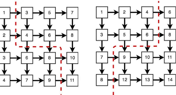
Deficiency of the ModelThe k-min cut model does not account forwait time. We de-finewait timeas the machine idle time when no task can execute because their dependency have not been satisfied. In Figure 2.1, we show that two partitions with the same overall communication cost can have very different makespans. Figure 2.1 uses a dependency graph similar to that of Recurrent Neural Networks (RNN) and assumes unit computation and unit communication time. The number in each node denotes their starting time given the partition marked by the dotted line in the image. As we can see, the left partition results in a much smaller makespan than the right partition, even though they have the same total communication cost. Since k-min cut only minimizes the communication cost, we conclude that it is not a suitable model for our problem.
Figure 3.1: The left and right partitions have the same communication cost but different makespans
3.3.2 Scheduling with Communication Delay
Alternatively, we model the placement problem as ascheduling with communication delay problem.
Scheduling with Communication Delay Model Given a dependency DAG G, the scheduling with communication delay problem schedules tasks on machines while accounting for communication delays between related tasks placed on different machines. The problem’s objective is to minimize the total execution time (makespan) of G. Since this model focuses on holistically minimizing the makespan instead of just concentrating on the communication time, it is better suited to the placement problem.
Variants of the problem The problem has three common variants. The unit com-putation time unit communication time (UET-UCT) version of the problem assumes unit computation time and unit communication time in the dependency graph G. The small communication time (SCT) version of the problem assumes that the ratio between the max-imum communication time between any two nodes and the minmax-imum computation time for any node is ≤ 1. The general version of the problem places no constraints on either com-munication or computation time.
NP-HardnessAs proven in [36], the problem is NP hard even when reasonable accom-modations are provided, such as infinite number of processors and UET-UCT conditions. Therefore, approximation algorithms are developed to provide a solution in polynomial time with good accuracy.
Existing Work Most approximation algorithms solve the scheduling with communica-tion delay problem with special assumptions such as UET-UCT or SCT. To the best of the author’s knowledge, no constant approximation ratio algorithm has been developed for the general scheduling with communication delay problem. For the general case, [37] describes an earliest task first (ETF) scheduling scheme which has the best known approximation ratio of 2 +ρ− 1
m,whereρ is ratio between the maximum communication time between any two nodes and the minimum computation time for any node in the graph andm is the total number of machines (for more details see section 4.2). Under the SCT constraint (ρ ≤1), algorithms with better approximation ratios are known. By using linear programming (LP) relaxation and priority based greedy scheduling, [17] is able to achieve an approximation ratio of 4+32+ρρ − m2+2(2+ρρ). Since ρ ≤ 1 under the SCT assumption, the approximation ratio is constant (for more details see section 4.3).
Viability of the SCT Assumption Neural Networks are computationally intensive as mentioned in chapter 1. This characteristic, coupled with the fact that distributed NN frequently utilize high performance computers in data centers (resulting in smaller commu-nication times), makes the SCT assumption viable. If for certain applications, the SCT assumption is significantly violated, a collocating scheme described in [38] can be applied at the pre-processing stage. Computationally small nodes are grouped together and treated as a single node to reduce ρ to near-SCT compliance.
CHAPTER 4: ALGORITHM DESIGN
In this chapter, we present the details of the three selected algorithms: topological sort, ETF [37] and SCT [17] algorithm to solve the scheduling with communication delay problem. We modify all three existing algorithms to incorporate the memory constraint per machine, resulting in modified algorithms m-TOPO, m-ETF and m-SCT. We assume the memory on all machines to be homogeneously distributed for the purposes of this thesis. We assume the total memory on any individual machine to beM. Furthermore we prove the approximation ratio of m-SCT.
We also model our memory constrained scheduling with communication delay problem with integer linear programming (ILP), which generates the optimal solution. For small to medium size graphs (up to 50 nodes), the results can be generated within a reasonable amount of time (at most a few hours). In the future, the optimal solution can be used to provide a baseline and measure the performance of our modified approximation algorithms.
4.1 TOPOLOGICAL SORT 4.1.1 Definition
Topological sort is a linear ordering of vertices in a DAG G, such that for each directed edge u→v, u comes beforev in the linear ordering.
4.1.2 Algorithm description
The existing topological sort algorithm [39] first topologically sorts the nodes in DAG G, then place nodes evenly on each machine.
4.1.3 Memory constrained version:
In our modified algorithm m-TOPO, we first number the total number of m machines from 1 to m. Then, we assign tasks to machines in increasing order. For any machine i, m-TOPO places nodes until a machine is full or the total number of nodes placed so far is ≥ in
4.2 ETF
4.2.1 Algorithm description
The existing earliest task first (ETF) algorithm [37] schedules the earliest schedule-able task first, and the process is repeated until all tasks are scheduled. The algorithm maintains a task list I with unscheduled tasks and a machine list P with the earliest time a machine becomes available. The next available time of each machine is denoted by f ree(p). The algorithm
1. computes the earliest schedule-able time for all tasks in I, 2. selects the task with the smallest earliest schedule-able time,
3. schedules the task from b on the machine where it can begin at the earliest.
For any task i, let si be the starting time and pi be the computation time. Let Γ−(i) be the set of all immediate predecessors of task i. For any edge i → j ∈ E(G), let cij be the communication delay between tasks i and j. cij is only valid when tasks i and j are on different machines. Denote xip to be 0 when task i is on machine p and 1 otherwise. The earliest schedule-able time for any task j (a) is min
p∈P
h
max f ree(p), max
i∈Γ−(i)(si+pi+cijxip) i
. Under the small communication time (SCT) assumption, ETF has approximation ratio 2 + ρ− 1
m, which tends to 3 when ρ approaches 2 and m is large. A detailed description can be found in [37].
4.2.2 Memory constrained version
In our modified algorithm m-ETF, at each step we sort the task machine pair (t, p) accord-ing to the taskt’s earliest schedule-able time on machinep. Then we examine task machine pairs in the sorted order, until we find (t, p) where adding taskt to machinepwill not result inp0s memory being overloaded.
4.3 SCT
1. Scheduling tasks together that are also scheduled together in the infinite machine variation of the problem, as described in the following section.
2. Scheduling an urgent task. An urgent task at time t is one that can be scheduled on any idle machine to begin at time t. Such a task has already been delayed scheduling and should not be further ignored.
When the above prioritizing scheme results in better approximation ratio with the SCT assumption. We describe below the algorithm in detail.
Infinite machine algorithm For the infinite number of machines case, the SCT as-sumption makes it possible to model the problem as an integer linear programming (ILP) with a meaningful linear programming (LP) relaxation. As discussed in the Reflection chap-ter (chapchap-ter 8), not all ILPs have meaningful LP relaxations.
The SCT assumption ensures that; for each task i, it is advantageous to schedule only one immediate successorj on the same machine as i. Scheduling two successors ofion the same machine as i is not optimal because the second task could have started earlier on a new machine. For any task i, a favorite child f(i) denotes the preferred successor of i that is scheduled on the same machine as i.
The ILP is formulated as follows,
minw∞ Minimize makespanw∞
∀i→j ∈E(G), xij ∈ {0,1} xij = 0 when j is i’s favorite child ∀i∈V(G), si ≥0 All tasks start after time=0 ∀i∈V(G), si+pi ≤w∞ all tasks should complete before
makespan
∀i→j ∈E(G), si+pi+cijxij ≤sj Given edge i→j, j must start after i completes. If on different machines, communication cost should be added
∀i∈V(G), X j∈Γ+(i)
xij ≥ |Γ+(i)| −1
Every node has at most 1 favorite child
∀i∈V(G), X j∈Γ−(i)
xij ≤ |Γ−(i)| −1
Every node is the favorite child of at most 1 predecessor
(4.1)
between 0 and 1. This LP can be solved in polynomial time using the interior point method [40]. Then the SCT algorithm simply rounds the LP solution xij to be 1 if xij ≥0.5 and 0 otherwise. It can be easily verified that the rounded solution complies with all constraints stated above. xij can be used to determine the favorite child of each task. j is i’s favourite child if and only if xij = 1.
This infinite machine algorithm achieves an approximation ratio 2+22+ρρ, as described in [17]. Finite machine algorithm The favourite child determined by the infinite machine case alongside the urgent task are used as priorities. Then priorities are incorporated into the base SCT algorithm to determine the final placement. In order to understand the algorithm, let’s consider a partially completed schedule S at an arbitrary time t during the execution. Letibe the last task scheduled on machinep. For each remaining unscheduled taskj, denote the machine on which j can start the earliest as ep(j). Let’s define a machine p to be free at time t if machine pis available at time t and it is possible to schedule i’s favourite child f(i) earlier on a different machine. In other words, ep f(i) 6= p. Let’s define a machine p to be awake at timet if it is favourable to schedule i’s favourite child on p. In other words, ep f(i) =p.
The algorithm maintains a listP of machines in the order of their earliest available time. Let’s consider a machinepthat is available at timet. Ifpisfree att, the algorithm schedules the earliest task available on p. If an urgent task is available, it will naturally also be the earliest task. If pisawake, the algorithm schedules an urgent task on pif there is an urgent task in I at time t, otherwise it schedules the favorite child f(i) ofi on p.
The algorithm repeatedly finds the next moment when a machine is available t, and schedules task on available machines as described above, until all tasks are scheduled.
If a task i and its favorite child f(i) are scheduled together in the infinite machine algo-rithm, it results in a very good approximation ratio. This intuitively shows that f(i) has a bigger influence on the start time of future tasks than i’s other successors and thus it is advantageous to schedule i and f(i) together even in the finite machine case. [17] proves that the SCT algorithm gives a better approximation ratio than ETF, as expected. The SCT approximation ratio is 4+32+ρρ − 2+2ρ
m(2+ρ) approximation ratio, which tends to 7
3 when ρ
approaches 1 and mis large, while the ETF approximation ratio approaches 3 (as described in section 4.2). See [17] for detail of the proof of the approximation ratio.
4.3.2 Memory constrained version
For our memory constrained version of the SCT algorithm (m-SCT), we maintain the same priority scheme as the finite case SCT algorithm. To enforce the memory constraint, we assume each machine has the same amount of memory M. Let K = PmMn
i=1di
, where m is the total number of machines, n is the number of nodes in graph G and for any node i inG, di is the size of memory required by i. Intuitively, K is the ratio of the total memory available from all machines to the total memory required by the model. When the memory M on a machine is exceeded, we drop it from the list of available machines for the duration of the algorithm. We prove below that m-SCT approximates the optimal solution within (1 + (2+2+2ρ)ρm)· 1
K−1 of the finite SCT’s approximation ratio.
Theorem 4.1 Let the approximation ratio given by the finite SCT algorithm be α, then m-SCT has approximation ratio ≤α+ (1 + (2+2+2ρ)ρm)· 1
K−1. Proof: Since M = K m n X i=1
di, from a total of m machines, at most mK machines would be full (hence dropped) at any time. Therefore, there are at least (K−1)K m machines not dropped throughout the algorithm.
Let’s denote w∞ as the makespan given by the infinite SCT algorithm and w∞OP T as the optimal solution to the infinite machine variation of scheduling with communication delay problem. Let wm
OP T be the optimal solution to the m machine finite scheduling with communication delay problem andwOP T mm be the optimal solution to the memory constrained m machine finite scheduling with communication delay problem. Then, w∞OP T ≤ wmOP T ≤ wmOP T m.
Since at least (K−1)K m machines are always available for scheduling in m machine m-SCT, it generates a makespan T0 at least as good as the one generated by finite SCT with (K−1)K m machines, T.
From [17], the m machine finite SCT algorithm has makespan W such that W ≤ 1
m ·
Pn
i=1pi+ (1− m1)w∞. Therefore, the (K
−1)m
T such that, T ≤ (K−1)1 m K · n X i=1 pi+ (1− 1 (K−1)m K )w∞ ≤ K (K−1)m n X i=1 pi+ (1− K (K−1)m)w ∞ = K K−1 1 m n X i=1 pi+ (1− K (K−1)m)w ∞ ≤ K K−1w m OP T + (1− K (K−1)m)w ∞
As described in section 4.3.1, the approximation ratio betweenw∞ andw∞OP T isβ = 2+22+ρρ. For the makespan T0 generated bym machine m-SCT,
T0 ≤T ≤ K K−1+ (1− K (K−1)m)β wOP T mm (4.2) ≤( 1 K−1 + β (K−1)m) + 1 + (1− 1 m)β wOP T mm (4.3) Themmachine finite SCT algorithm in [17] has the approximation ratioα= 1 + (1− 1
m)β. Using equation (4.2), m-SCT has an approximation ratio α+ (1 + (2+2+2ρ)ρm)· 1
K−1.
4.4 OPTIMAL SOLUTION
We modified the infinite machine ILP (described in section 4.3.1) to incorporate the finite machine and memory constraints. [41] [42] [43] [44] show other similar attempts in the area. Through this section, let V be the set of all tasks and E be the set of all edges in G, the dependency graph.
4.4.1 Memory constraints
In this section, we discuss how to incorporate memory constraints in the infinite machine SCT constrained ILP formulation. In this ILP, no variable records which machine a task is placed on. However, for enforcing the memory constraint, we must record the tasks associ-ated with each machine. Let yip be 1 if task i is on machine p and 0 otherwise. Let mi be
machine can be modeled as follows, ∀p∈P, n X i=1 yipmi ≤M (4.4)
We need a variablexij, which describes whether taskiand taskj are on the same machine for our ILP. Let xij be 1 if i, j are scheduled on the same machine and 0 otherwise. Then xij = 1, if and only if for some machine p, yipyjp = 1 (both i and j are on machine p). Therefore, we modelxij as,
xij =
X
p∈P
yipyjp (4.5)
However, (4.4) is not linear and cannot be added to an ILP. We now attempt to linearize (4.4). Let’s define yijp = yipyjp. Now, xij and yijp have a linear relationship. Fortunately, since yip and yjp are both boolean variables, we can further express yijp’s relationship with yip and yjp using linear equations. Namely,
yijp≥yip+yjp−1 yijp≤yip
yijp≤yjp (4.6)
yijp∈ {0,1}
This linear model ensures that yijp is true if and only if both i and j are on machine p, i.e., yijp = 1 whenyip = 1 andyjp = 1 and 0 otherwise. Combining the equations above, the following equations model the memory constraints in totality,
∀p∈P, n X i=1
yipmi ≤M Total memory on each machine≤M ∀i, j ∈V, xij =
X
p∈P yijp
Tasks i and j are on the same machine when for some machine p, both i and j are on machine p
∀i, j ∈V, p∈P, yijp ≥yip+yjp−1 If both yip and yjp = 1, then both task i and j are on machine p and yijp= 1
∀i, j ∈V, p∈P, yijp ≤yip yijp= 1 only when i is on machine p ∀i, j ∈V, p∈P, yijp ≤yjp yijp= 1 only when j is on machine p ∀i, j ∈V, p∈P, yijp ∈ {0,1} Whether both i and j are on machine p ∀i∈V, p∈P, yip ∈ {0,1} Whether i is on machine p
∀i, j ∈V, xij ∈ {0,1} Whether i and j are on the same machine.
(4.7)
4.4.2 Finite machine constraints
In this section, we model the required finite machine constraints with linear equations. Let’s define tasks i and j to be unrelated when task i is not an ancestor of task j and task j is not an ancestor of task i. An important difference introduced by the finite machine constraint is that we may have to put unrelated tasks on the same machine because of the limited number of total machines. In the original infinite machine SCT constrained ILP, there is no constraints specifying the relationship of unrelated tasks’ starting time, since they would never be placed on the same machine. Here, if twounrelated tasks are scheduled on the same machine, we must additionally ensure that the execution time of the tasks do not overlap. This can be modeled as an additional constraint,
si+pi ≤sj OR sj +pj ≤si (4.8) where for any task i, si is the starting time of taski and pi is the computation time of task i. Equation (4.5) ensures that either task iis fully executed before task j’s starting time or vice versa. This is important because it is not possible to parallelly execute tasks on a single machine. It is possible to convert the above nonlinear constraint into a linear form. Let’s define bij = 0 when task i executes before task j and 1 otherwise. Then, equation (4.5) is
equivalent to the following constraints,
si−sj ≤ −pi+ (U +pi)bij (4.9)
si−sj ≥L+ (pj −L)bij (4.10)
Intuitively, when bij = 0, then i executes before j, and (4.6) enforces that i’s execution must finish beforej’s starting time. In this case, (4.7) is always true and does not interfere. When bij = 1, (4.7) similarly ensures that j’s execution must finish before i’s starting time. In this case, (4.6) is always true and does not interfere. We choose constants L and U to appropriately activate which constraint dominates in each case. One way to choose L and U is to set L =−(P i∈V pi+ P i→j∈Ecij) and U = P i∈V pi+ P
i→j∈Ecij. Therefore, when bij = 0, i is completed before j starts.
We must only enforce constraints (4.6) and (4.7) when tasks i and j are on the same machine. This leads to a slight modification to constraints (4.6) and (4.7), as we incorporate xij (as defined in section 4.4.1), which is a boolean variable describing whether tasks i and j are on the same machine, as follows,
∀(i, j)6∈E, si−sj ≤ −pi+ (U+pi)(bij + 1−xij) (4.11) ∀(i, j)6∈E, si−sj ≥L(2−xij) + (pj−L)bij (4.12)
4.4.3 Final ILP formulation
Summarizing the above constraints for finite memory and number of machines, and com-bining them with the infinite machine ILP (described in section 4.3.1), we arrive at the final ILP.
minw Minimize makespan
∀i∈T, si ≥0 All tasks start sometime after 0 ∀(i, j)∈E, xij ∈ {0,1} Whether i and j are on same machine ∀i∈T, si+pi ≤w All tasks complete before makesapn ∀(i, j)∈E, si+pi+ (1−xij)cij ≤sj j must start after i completes and if
they are on different machines
∀i∈V, p∈P, yip ∈ {0,1} Whether i is on machine p
∀i, j ∈V, p∈P, yijp ∈ {0,1} Whether both i and j are on machine p ∀i∈V,X
p∈P
yip= 1
Each task should be scheduled on exactly 1 machine
∀i, j ∈V, p∈P, yijp ≥yip+yjp−1 If both yip and yjp = 1, then both i and j are on machine p and yijp= 1 ∀i.j ∈V, p∈P, yijp ≤yip yijp= 1 only when i is on machine p ∀i, j ∈V, p∈P, yijp ≤yjp yijp= 1 only when j is on machine p ∀i, j ∈V, xij =
X
p∈P yijp
Tasks i and j are on the same machine when for some machine p, both i and j are on machine p ∀p∈P, n X i=1 yipsi ≤M
Total memory used on each machine ≤M
∀(i, j)6∈E, si−sj Enforces that when bij = 0, i finishes ≤ −pi+ (U+pi)bij +U(1−xij) before j starts, given that i, j are on
the same machine (xij = 0). If i and j are on different machines, constraint becomes meaningless and degrades to their starting time difference being less than an arbitrary large number U ∀(i, j)6∈E, si−sj Enforces that when bij = 1, j finishes ≥L+ (pj−L)bij +L(1−xij) before i starts, given that i, j are on
the same machine (xij = 0). If i and j are on different machines, constraint becomes meaningless and degrades to their starting time difference being larger than an arbitrary small number L
CHAPTER 5: BACK PROPAGATION
In this chapter, we discuss how to account for back propagation in the algorithms proposed in chapter 4 and prove certain makespan and approximation ratio guarantees for it.
5.1 DEFINITION AND NEED FOR BACK PROPAGATION
DefinitionIn neural network training, the back propagation algorithm (a) propagates the total error backwards through the Neural Network (NN) layers (b) computes the gradient of each weight and bias in the network, using the propagated error (c) applies the gradients calculated in (b) to their corresponding weights and biases (d) eventually minimizes the total error of the NN.
Need for BP The back propagation algorithm is needed to train multi-layer NNs. It corrects the weights and biases of every layer in the NN to reduce the error in each iteration of the training process.
5.2 ACCOUNTING FOR BACK PROPAGATION
The scheduling algorithms discussed in chapter 3 are only valid for directed acyclic graphs. The process of backpropagation in NN training introduces some cycles and is computation-ally intensive. Since BP is non trivial and accounts for a significant chunk of the makespan, we account for it separately.
5.3 SCHEDULING STRATEGY
Each operation node in TensorFlow (TF) has an associated gradient node that is re-sponsible for the calculation of gradient for that operation. Similarly, each variable has an associated GradientDescent node whose primary purpose is the application of gradient and updating the variable. Together, these two nodes are primarily responsible for the BP process. Between these two functionalities, gradient computation accounts for the majority of the complexity.
If we collocate thegradient nodes with their corresponding operation nodes, we discover that the resulting backward dependency graph G0 is the reverse of the forward propagation graphG, i.e., same vertices and reverse edges. TF provides a very straightforward interface to
specify these collocations. Unlike thegradient nodes, which must wait for their predecessors from G0 before executing, the GradientDescent nodes have no such dependencies. The gradient application can be carried out at any time in the BP process after the gradient has been calculated for a node, including at the end. Given the lack of GradientDescent node inter-dependencies and their less intensive nature, their contribution to the makespan can be safely ignored for the purposes of our proofs. Their withdrawal from consideration serves another critical purpose. Without the GradientDescent nodes, the connections between the forward and backward computation graphs (G andG0) are severed and the entire NN graph can be considered a DAG. Under this assumption, our previously discussed algorithms from chapter 4 can be successfully used.
5.4 GUARANTEES
Given the assumptions stated above, we prove certain guarantees for the BP phase in the remainder of this chapter. First, we show that the makespan of the backward pass is within C0 (as defined in section 5.4.1) times the makespan of the forward pass. Next,
we prove that if C (as defined in section 5.4.1) is constant across the NN, the initially established approximation ratio remains unchanged after back propagation. It is worth noting that while the makespan guarantee only holds if the gradient nodes are collocated with operations, in practice, it is possible to apply DAG algorithms simply after the removal of the GradientDescent nodes.
5.4.1 Preliminaries
In this subsection, we define a schedule and enumerate the necessary and sufficient condi-tions for a schedule to be legal.
Schedule We define a schedule S for graph G as a list that associates each node in G with a machinep on which it will be executed and a starting time si.
Backward ScheduleDenote the makespan of scheduleS asT. We define forward sched-ule S’s corresponding backward scheduleS0 as a schedule where for any nodei inG, (a) iis associated with the same machine as inS (b)i has starting times0i =C0(T−si−pi), where s is i’s starting time inS.
Legal ScheduleLet’s denote the computation time of nodei in dependency graph G as pi and the communication time between any two tasksi and j in G to be cij.
Schedule S is legal if and only if, 1. si ≥0
2. si +pi ≤ sj or sj +pj ≤ si when task i and task j are on the same machine. This guarantees that tasks i and j do not overlap.
3. si+pi ≤sj when taskiand taskj are on the same machine and there is an edge i→j in the dependency graphG. This guarantees that the precedence relationship between tasksi and j is honored, when they are on the same machine.
4. si+pi+cij ≤sj when taski and taskj are on different machine, and there is an edge i → j in the dependency graph G.cThis guarantees that the precedence relationship between tasksi and j is honored, when they are on different machines.
Backward dependency graph The backward dependency graph G0 is the reverse of the forward propagation graph G, i.e., G0 shares the same vertices with G but has reversed edges. We denote the computation time of a nodej inG0 asp0j and the communication time between any nodes j and iin G0 asc0ji.
NN proportionality constantWe define the NN proportionality constantC0for forward
graphGand backward graphG0 as the maximum ratio between (a) corresponding backward pass edge weight and forward pass edge weight and (b) corresponding backward pass node weight and forward pass node weight.
C0 =max maxj∈V(G) p0j pj, maxi→j∈E(G) c0ji cij
NN proportionality functionWe define the NN proportionality function C as follows (a) For any nodei∈V(G), letC(i) = p0i
pi (b) for any edgei→j ∈E(G), letC(i→j) =
c0ji cij.
We say function C is constant if for all i ∈ V(G), C(i) = C0 and for all i → j ∈ E(G),
C(i→j) =C0. Essentially, C0 is the max over all values of C.
5.4.2 Theorems
Theorem 5.1 Given a scheduleS onG, S’s corresponding backward scheduleS0 is legal and makespan(S0)≤C0·makespan(S)
Proof We know that ∀i→j ∈E(G), c0ji ≤C0cij and ∀j ∈V(G), p0j ≤C0pj Denote the makespan of scheduleS asT.
We prove below that the scheduleS0 is legal: 1. We know T ≤si+pi∀i
Therefores0i =C0(T −si−pi)≥0 ∀i∈V(G)
2. Let i, j be 2 arbitrary tasks assigned to the same machine.
Since S is a legal schedule, we know that si+pi ≤sj orsj +pj ≤si. T −si−pi ≥T −sj−pj+pj or T −sj−pj ≥T −si−pi+pi.
C0(T −si−pi)≥C0(T −sj−pj) +C0pj orC0(T −sj−pj)≥C0(T −si−pi) +C0pi.
s0i ≥s0j +p0j ors0j ≥s0i+p0i.
3. Let j →ibe an arbitrary edge in G0 and i, j are assigned to the same machine inS. i→j ∈E(G)<=> j →i∈E(G0).
Since S is a legal schedule, we know that i→j ∈E(G), si+pi ≤sj. C0(T −si−pi)≥C0(T −sj −pj) +C0pj.
s0i ≥s0j +p0j inG0.
4. Let j →ibe an arbitrary edge in G0 and i, j are assigned to different machines. i→j ∈E(G)<=> j →i∈E(G0)
Since S is a legal schedule, we know that i→j ∈E(G), si+pi+cij ≤sj. C0(T −si−pi)−C0ci→j ≥C0(T −sj −pj) +C0pj.
C0(T −si−pi)≥C0(T −sj −pj) +C0pj +C0cij. s0i ≥s0j +p0j +c0ji inG0.
S0 satisfies all condition for a legal schedule and therefore is legal.
makespan(S0) = maxi(s0i+p0i) =maxi(C0(T −si))≤C0T =C0·makespan(S)
Theorem 5.2 When NN proportionality function C is constant, the makespan of optimal schedule for G0 isC0 times the makespan for optimal schedule for G.
Proof We know that ∀j ∈V(G0),p
0 j
pj =C0, and ∀j →i∈E(G
0),c0ji
cij =C0.
Therefore,maxmaxj∈V(G0)pj
p0 j , maxj→i∈E(G0)cij c0 ji = C1 0.
Let OP T be the shortest makespan for any schedule on G with m machines. Let S∗ be an optimal schedule forG.
By Theorem 5.1 we know that there is a schedule S0 for G0 where makespan(S0) ≤ C0makespan(S∗), therefore OP T0 ≤makespan(S0)≤C0makespan(S∗) =C0OP T.
For the same reasonOP T ≤ 1
C0OP T 0.
Therefore OP T0 =C0OP T.
Theorem 5.3 When NN proportionality function C is constant, given a schedule S for G, the backward schedule S0 has the same approximation ratio as S.
Proof By Theorem 5.2, the makespan of optimal schedule for G’ OP T0 is C0 times the
makespan for optimal schedule OP T for G.
By Theorem 5.1,makespan(S0)≤C0makespan(S) andmakespan(S0)≤ C10makespan(S).
makespan(S0) = C0makespan(S).
Therefore, makespanOP T0(S0) =
makespan(S)
OP T , which means the approximation ratio of S
0 equals
CHAPTER 6: IMPLEMENTATION
In this chapter, we provide implementation and simulation details of our selected algo-rithms. We resort to using the simulation technique as it allows for easy comparison of algorithms without committing to any framework and being influenced by the idiosyncrasies of any specific implementation.
6.1 SIMULATION
We implement the algorithms discussed in chapter 3 in NetworkX [45], a popular open source Python package for creation and manipulation of graphs. In order to compare all the algorithms and demonstrate the difference in their efficiencies effectively, we simulate distributed graph partitioning. We test our selected algorithms on Inception-V3 [46] and a small custom Convolution Neural Network (CNN) [47] graph model (described in greater detail in chapter 6). These graphs are good representations of commonly used models in Machine Learning (ML) frameworks, such as TensorFlow. For the simulation, first, we realis-tically estimate the computation time of each node and the inter node communication times. Then, we create a new graph in NetworkX where each node corresponds to a computation task from the selected model (with its weight being the computation time) and each edge corresponds to the dependency between these tasks (with the edge weight being the inter node communication time). Finally, we execute the selected algorithm on this graph, which yields the placement and the corresponding makespan.
6.2 ESTIMATION OF COMPUTATION TIME
To estimate the computation time we input a model into TensorFlow and generate the graphdef, an internal representation of the TensorFlow (TF) graph and part of its core framework (as described in section 2.1). The graphdef is then profiled using a TF python client, timeline, which outputs a JSON file. The JSON file details the computation time of each TF node as a dur argument as can be seen from figure 5.1. In order to avoid the initialization costs, we use the computation data from the 50th iteration and experimentally verify that the computation time for further iterations is approximately the same. The nodes which do not have any computation time associated with them and exist merely for
in figure 5.2.
It’s worth noting that the TF graph is different from the logical graph as it includes nodes for variables, operations and several other ancillary nodes like read/write (as detailed in section 2.1). The use of the TF graph is preferable to the logical one as it gives substantial insight into how Machine Learning frameworks break down logical operations and establish the control flow. Simulation using this real world breakdown of nodes is more likely to yield realistic results that can be extrapolated to other existing Machine Learning systems as well.
Figure 6.1: Timeline [8] output for a vari-able with computation time of 3ms
Figure 6.2: Timeline [8] visualization
6.3 ESTIMATION OF COMMUNICATION TIME
The inter node communication time factors significantly in all our scheduling algorithms. To estimate the communication time effectively, if two nodes are on the same machine, we assume communication time to be zero. This assumption is justified because communication over a network is many times more expensive than within the same machine. For all other cases, first, the total size of the data to be communicated is determined using equation (5.1). We obtain the tensor dimensions in a similar way as the computation times, using the time-line object. The JSON file obtained in this case provides the tensor description argument which lists the dimensions of the tensor as well as the total bytes requested by the system for that tensor (based on its datatype) as shown in figure 5.3.
Figure 6.3: Timeline [8] output for tensor of dimensions 100,784 requesting 313600 bytes of memory
Once the size of tensor is determined and we assume a suitable network bandwidth, the communication time is calculated based on equation 5.2. We use a variety of bandwidths in our experiments in order to see how performance varies as the data centre bandwidth varies. Greater bandwidths imply smaller communication time, and help comply with the small communication time (SCT) assumption better (see section 4.3.2).
Communication time = size/bandwidth (6.2) Sometimes in TF, the size of the tensor is dynamically determined at run-time. Our models do not use any dynamic tensors as they are not conceptually different from the statically sized ones. Different techniques may be required to extract the size information for these cases in the future.
6.4 CONSTRAINTS
In the simulation, we introduce memory constraints on every processor and perform exper-iments using a fixed number of processors for each case. We vary the number of processors across experiments to note the makespan and partitioning trends as the number of processors change for different algorithms.
Unlike our simulation, TF has arbitrary rules about collocation of certain nodes on the same machine. These rules help assist the particular implementation architecture of TF and make it more productive. This is especially true in the case of backpropagation. Gradient
they deem fit. In the future, if TF experiments are carried out on similar models, some adjustments must be made to accommodate the collocation constraints.
6.5 LINEAR PROGRAMMING SOLVER
We use interior point method to solve the linear programming (LP) problems resulting from our algorithm. This method is preferred over other solvers such as simplex [48] be-cause it guarantees polynomial execution time [49]. Specifically, we use the primal dual interior-point solver in Mosek optimization software [50], which has a run time complexity of O(n3.5L), where L is the maximum number of bits in the LP inputs (in our case 64, the
number of bits in a python floating point number).
Experimentally, Mosek interior point solver is very fast, even for large graphs such as Inception-v3. For the Inception-v3 experiments in chapter 7, the Mosek interior point solver solves each LP in 3-10 seconds (see more details in chapter 7).
CHAPTER 7: EXPERIMENTAL RESULTS
In this chapter, we compare and contrast the performance of our selected algorithms on Inception-V3 and the small CNN model, and present our experimental results. For all our experiments, we assume a high speed data-center network (varying bandwidths) with no packet loss. We carry out the experiments on a Google VM machine (n1-standard-4 machine with 4 vCPUs and 15 GB memory).
The experiments are divided into two major categories; the fixed total memory experi-ments, where the total memory in the system remains constant regardless of the number of machines used, and the variable total memory experiments, where each machine has a fixed amount of memory and the overall memory of the system increases as the number of machines increase.
7.1 FIXED TOTAL MEMORY EXPERIMENTS
For the experiments in this section, we fix the total memory, which is distributed evenly across machines. As the number of machines increase, the memory per machine decreases.
7.1.1 Experiment on small CNN
SummaryIn this experiment, we compare m-TOPO, m-ETF and m-SCT’s makespan for the small Convolutional Neural Network (CNN) graph. We present the plots for these cases in Figure 7.1 to Figure 7.4.
Specifications We fix the total memory across all machines to be 3 times the memory required by the CNN, distributed evenly across machines. We vary the bandwidths (1E5, 1E7, 1E9 and 1E11 bytes/second ) and the number of machines (3, 6, 9, 12, 15) for all three alogorithms.
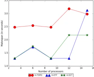
Trends and discussionIn the first three cases (Figure 7.1 to 7.3), the makespans of m-SCT and m-ETF algorithms display a gradually increasing trend as the number of machines increase. This behaviour can be attributed to the fact that the small CNN model is not very parallizable and the memory constraint becomes tighter as the number of machines increase.
increasing bandwidths because it leads to smaller inter-node communication times for them and both of them have a constant approximation ratio under the small communication time (SCT) assumption.
Across all cases, m-ETF and m-SCT steadily outperform m-TOPO, except for a few configurations where m-TOPO chances upon an optimal placement.
In the first three plots, m-SCT has more consistent performance than m-ETF because it prioritizes the placement of favorite children and urgent tasks. Under tight memory constraints, like in this experiment, the effect of these optimizations is very pronounced. Very few tasks can fit on a single machine and SCT chooses these more carefully than m-ETF. In the last case (Figure 7.4), the 1E11 bytes/second bandwidth is so large for the small CNN graph that the communication time is negligible. Therefore, the differences between the performances of m-ETF and m-SCT are not very significant.
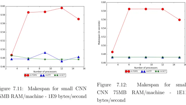
Figure 7.1: Makespan for small CNN with fixed total memory - 1E5 bytes/second
Figure 7.2: Makespan for small CNN with fixed total memory - 1E7 bytes/second
Figure 7.3: Makespan for small CNN with fixed total memory - 1E9 bytes/second
Figure 7.4: Makespan for small CNN with fixed total memory - 1E11 bytes/second Fixed total memory on small CNN
7.1.2 Experiment on Inception-V3
SummaryIn this experiment, we compare m-TOPO, m-ETF and m-SCT’s makespan for the Inception-V3 model. We present the plots for these cases in Figure 7.5 to Figure 7.8.
Specifications We fix the total memory across all machines to be 3 times the memory required by the Inception-V3 model. We vary the bandwidths (1E7, 1E9, 1E10 and 1E11 bytes/second ) and the number of machines (3, 6, 9, 12, 15) for all three algorithms.
Trends and discussion For the E7 bytes/second bandwidth case (Figure 7.5), m-SCT performs poorly because the because the bandwidth is very low and the SCT assumption is significantly violated (as communication times become larger due to low bandwidth). As the bandwidth increases in the subsequent cases (Figure 7.6 to 7.8), m-SCT behaves better and outperforms both m-ETF and m-TOPO.
Across all cases (Figure 7.5 to 7.8), the makespan of m-SCT dips to a low point and rises afterwards. As the number of machines increase, the availability of free machines that can execute a ready task also increases. In this scenario, there are fewer than usualurgent tasks that are waiting to be executed and the m-SCT algorithm loses some of its advantage over
perform m-TOPO, similar to the CNN experiment.
We notice that the total memory constraint in this experiment (three times the required memory) is not very high. We expect that if this constraint is tightened further, the perfor-mance difference between m-ETF and m-SCT will become more pronounced.
Figure 7.5: Makespan for InceptionV3 -fixed total memory - 1E7 bytes/second
Figure 7.6: Makespan for InceptionV3 -fixed total memory - 1E9 bytes/second
Figure 7.7: Makespan for InceptionV3 -fixed total memory - 1E10 bytes/second
Figure 7.8: Makespan for InceptionV3 -fixed total memory - 1E11 bytes/second Fixed total memory on Inception-V3
7.2 VARIABLE TOTAL MEMORY EXPERIMENTS
For the experiments in this section, we fix the total memory on each machine. The total memory in the system increases as the number of machines increase.
7.2.1 Experiment on small CNN
SummaryIn this experiment, we compare m-TOPO, m-ETF and m-SCT’s makespan for the small CNN graph. We present the plots for these cases in Figure 7.9 to Figure 7.12.
Specifications We fix the memory of an individual machine as 75 MB. We vary the bandwidths (1E5, 1E7, 1E9 and 1E11 bytes/second) and the number of machines (3, 6, 9, 12, 15) for all three algorithms.
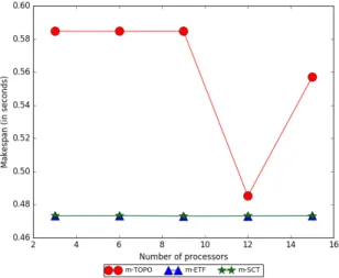
Trends and discussion Across all cases (Figure 7.9 to 7.12), m-ETF and m-SCT out-perform m-TOPO, as expected.
Both m-SCT and m-ETF display a generally decreasing trend as the number of machines increase. The performance of m-ETF improves significantly with the increase in the number of machines as the tight memory constraint (from fewer machines) penalizes m-ETF heavily for not smartly prioritizing the placements of any tasks. For high number of machines, the effects of prioritizing become less prominent as machines become less crowded and many related tasks can easily fit on the same machine without making an extra effort to schedule them together. This behaviour is observed for all bandwidths.
Figure 7.11: Makespan for small CNN 75MB RAM/machine - 1E9 bytes/second
Figure 7.12: Makespan for small CNN 75MB RAM/machine - 1E11 bytes/second
Variable total memory on small CNN
7.2.2 Experiment on Inception-V3
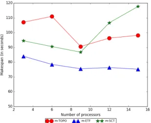
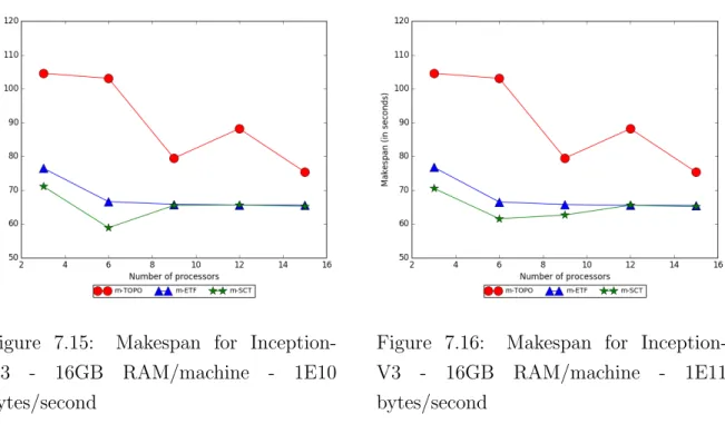
SummaryIn this experiment, we compare m-TOPO, m-ETF and m-SCT’s makespan for the Inception-V3 graph. We present the plots for these cases in Figure 7.13 to Figure 7.16. SpecificationWe fix the memory of an individual machine as 16 GB. We vary the band-widths (1E7, 1E9, 1E10 and 1E11 bytes/second) and the number of machines (3, 6, 9, 12, 15) for all three algorithms. The Inception-V3 model is tested on a subset of imagenet (flower). Trends and discussion Across all cases (Figure 7.9 to 7.12), m-ETF and m-SCT out-perform m-TOPO, as expected.
Both m-SCT and m-ETF display a generally decreasing trend. This behaviour is very similar to the CNN experiment (section 7.2.1). The imagenet dataset can result in some very large tensor sizes for Inception-V3. When the bandwidth is as low as 1E7 bytes per second (Figure 7.13), the SCT assumption is severely violated and the priorities determined by m-SCT are not very accurate. In this case, m-ETF performs better than m-SCT because (a) the steadily increasing memory benefits m-ETF, as explained in section 7.2.1. (b) m-SCT uses inaccurate priority.
accurate and m-SCT starts outperforming m-ETF as expected.
Figure 7.13: Makespan for InceptionV3 -16GB RAM/machine - 1E7 bytes/second
Figure 7.14: Makespan for InceptionV3 -16GB RAM/machine - 1E9 bytes/second
Figure 7.15: Makespan for Inception-V3 - 16GB RAM/machine - 1E10 bytes/second
Figure 7.16: Makespan for Inception-V3 - 16GB RAM/machine - 1E11 bytes/second
Variable total memory on Inception-V3
cases (as long as the SCT assumption is not violated, which can happen at low bandwidths) and is significantly better performing than m-TOPO and m-ETF when memory is tightly constrained.
CHAPTER 8: REFLECTION
In this chapter we describe our unsuccessful attempts at approximating the solution to the optimal ILP formulation, modeling the memory constrained finite machine scheduling with communication delay problem, using a pure LP relaxation approach. We present the challenges and the reasons for failure of this method.
8.1 APPROXIMATION OF THE ILP SOLUTION
As illustrated in section 4.4, the optimal solution integer linear programming (ILP) opti-mally models the objective function and constraints for the memory constrained scheduling with communication delay problem. However, solving this optimal ILP is an NP hard prob-lem and requires exponential time. We attempt to use the linear programming (LP) relax-ation technique on the optimal ILP formulrelax-ation (described in section 4.4) in order to obtain an approximate polynomial time solution to our problem. To formulate an optimal solution, we modify the infinite machine ILP [17] by incorporating finite machine and memory con-straints. When we attempt to relax the additional constraints (to an LP) individually, we are faced with a unique set of challenges for each case. We describe them below in further detail.
8.1.1 Challenges in the finite machine constraints relaxation
In this section, we show that LP relaxation of ILP constraints (4.11) and (4.12), which model the finite machine assumptions, is not meaningful.
As discussed in section 4.4.2, under the finite machine assumption, it is possible for the ILP to schedule twounrelated tasks on the same machine. Let tasks iand j be twounrelated tasks. If i and j are scheduled on the same machine, then either i is executed before j, or j is executed before i. This results in an OR condition, as seen in equation (4.8). In the remainder of this section we reason that OR constraints are non convex and show that this non convexity renders the relaxation of the finite machine constraints meaningless.
When a solution set S is convex, if a, b ∈ S, then any of their convex combination c = λa+ (1−λ)b for some non-negative λ, must belong to the set S. For an OR condition in the form x≤L OR x≥H(L < H),x=Land x=H are feasible solutions. However, most
One of the properties of LP is that its feasible region is always convex. Here, we are forced to relax the non convex solution space to a convex solution space, which is problematic. In the OR condition example above, the LP solution space would contain all x such that L < x < H, which the OR constraint should have excluded. In our case, equations (8.1) and (8.2) model the OR constraint as specified in section 4.4.2. To recap,
si−sj ≤ −pi+ (U +pi)bij (8.1)
si−sj ≥L+ (pj −L)bij (8.2)
In the ILP formulation, bij is a boolean variable that takes the value of either 0 or 1. After LP relaxation, bij is allowed to take any real value between 0 and 1. This implies that si −sj is able to take any real value between −pi and pj, which further implies execution overlap between task i and j, exactly what we hope to avoid. For instance, when bij = 0.5, si−sj ≥
L+pj
2 OR si−sj ≤
U−pi
2 . SinceL is a very small negative number and U is a very
large positive number, by equation (4.9) and (4.10), si−sj ≥ a small negative numberOR si−sj ≤a large positive number. In this casesi−sj = 0 is a feasible solution, indicating that tasks iand j will start at the same time on the same machine (an unacceptable result). To conclude, LP relaxation does not accurately approximate the ILP finite machine constraints.
8.1.2 Challenges in the memory constraints relaxation
In this section we discuss the challenges associated with meaningfully rounding the LP relaxation of the ILP memory constraints, due to the presence of many interdependent variables. From section 8.1.1, we know that for the finite machine case, a pure LP relaxation approach is infeasible. The LP must be supplemented by greedy scheduling in this case. We conclude that it is preferable to enforce the memory constraints in the greedy portion of the combined algorithm.
The linear equations based on the memory constraints introduce many highly correlated variables, which makes independent rounding hard. For example, in the final optimal ILP formulation (4.4.3), yijp is dependent on yip and yjp. Furthermore xij is dependent on yijp. If we independently roundyip, then we cannot also independently roundyijpand xij without violating some of the LP constraints. Moreover, independent rounding must satisfy the memory constraint per machine (M) presented in equation (8.3) and recapped below,
∀p∈P, n
X
i=1
In the LP relaxation of (8.3),yip is allowed to take any value between 0 and 1. It is highly likely thatyipwill take some fractional value. After we obtain a solution to the LP relaxation problem, we must round the value of yip to 0 or 1 to satisfy the original ILP constraints. In the rounding process, if multiple fractional yips are rounded up to 1, it is possible that equation (8.3) is no longer satisfied and the total memory required of machine pexceedsM. It is possible that with a complicated rounding scheme we could circumvent both of these issues, however, to the author’s knowledge, no existing rounding scheme handles complicated correlation between variables and still results in a good approximation ratio. Alternatively, if we use LP relaxation + greedy scheduling approach, we can shift the burden of enforcing the finite machine as well as the memory constraints to the greedy portion of the algorithm and relax the infinite machine ILP to LP without any issues. This solution, combined with the small communication time (SCT) assumption, results in the m-SCT algorithm as described in section 4.3.
8.2 FUTURE DIRECTIONS
Our main roadblock is that no convex optimization approach can relax a non convex constraint. Advancements in the field of non convex optimization may help generate better algorithms for our placement problem. It may also be possible that the existing constraints be expressed or relaxed in novel ways to avoid the non convexity.
![Figure 2.1: Model distributed across GPU 1 and GPU 2 to demonstrate model paralleli [4]](https://thumb-us.123doks.com/thumbv2/123dok_us/10116457.2912202/13.918.118.802.496.755/figure-model-distributed-across-gpu-demonstrate-model-paralleli.webp)
![Figure 6.1: Timeline [8] output for a vari- vari-able with computation time of 3ms](https://thumb-us.123doks.com/thumbv2/123dok_us/10116457.2912202/36.918.491.809.350.551/figure-timeline-output-vari-vari-able-computation-time.webp)