Methodology Used to Evaluate Computer Vision Algorithms in Adverse Weather Conditions

Transportation Research Procedia 14 ( 2016 ) 2178 – 2187

2352-1465 © 2016 The Authors. Published by Elsevier B.V. This is an open access article under the CC BY-NC-ND license (http://creativecommons.org/licenses/by-nc-nd/4.0/).

Peer-review under responsibility of Road and Bridge Research Institute (IBDiM) doi: 10.1016/j.trpro.2016.05.233

ScienceDirect

6th Transport Research Arena April 18-21, 2016

Methodology used to evaluate computer vision algorithms in

adverse weather conditions

PierreDuthon

_{*, Frédéric Bernardin}

_{, Frédéric Chausse}

_{, Michèle Colomb}

Cerema, 8-10, rue Bernard Palissy - 63017 Clermont-Ferrand Cedex 2, France

b

Université Clermont Auvergne, Université d'Auvergne, Institut Pascal, BP 10448, F-63000 CLERMONT-FERRAND, FRANCE

c_{CNRS, UMR 6602, IP, F-63178 Aubière, FRANCE}

Abstract

Computer vision systems are increasingly present in road environments. These have not been evaluated in adverse weather conditions, particularly in rain. The objective of this article is to develop tools to validate these computer vision systems in such adverse weather conditions. This study begins by setting up a digital rain image simulator based on a set of physical laws. In addition to the simple visual effect, it makes it possible to obtain images of rain displaying physical reality. The simulator was then validated against data acquired in the Cerema R&D Fog and Rain platform. Finally, a protocol is proposed to evaluate the robustness of image features in rainy conditions. This protocol was then used to test the robustness of the Harris image feature in these conditions. Thanks to the protocol established, the study concludes that the rain has an impact on this conventional feature. © 2016The Authors. Published by Elsevier B.V..

Peer-review under responsibility of Road and Bridge Research Institute (IBDiM). Keywords:Computer vision; adverse weather conditions; road safety; rain simulator; fog

1. Introduction

Cameras are increasingly present in road environments. Installed on infrastructure and sometimes associated with computer vision algorithms, they are used to optimize travel and make it safer. Amongst other tasks, they perform

* Corresponding author. Tel.: +3-347-342-1069; fax: +3-347-342-1001. E-mail address:[email protected]

© 2016 The Authors. Published by Elsevier B.V. This is an open access article under the CC BY-NC-ND license (http://creativecommons.org/licenses/by-nc-nd/4.0/).

automatic incident detection and traffic management. Car equipment manufacturers also say that they will be developed on vehicles in the coming years. Cameras will then allow the vehicle environment to be detected and understood, initially for advanced driver assistance systems (ADAS) and later for autonomous driving.

Currently, the analysis of the robustness of these computer vision systems is evaluated mainly in clear weather. Little research focuses on the impact of adverse weather conditions such as rain, fog, or snow. And yet this impact is capital in terms of safety, as computer vision systems must remain reliable even in these adverse conditions. Taking these conditions into account is particularly important as they are already critical in terms of safety for other reasons: limited skid resistance or reduced human perception.

The study presented here aims to evaluate the performance of computer vision systems in the particular case of rain. Artificial vision systems include the entire chain of image acquisition (by camera) to the final application via various algorithms. Computer vision algorithms conventionally employed in this field use image features before performing higher-level processing. Image features, an essential building block for computer vision systems, will be tested with three methods involving rain: digitally simulated rainfall on images, rain generated in the laboratory and real rain in the natural environment. In this article, rain in the natural environment is not addressed. Before one can evaluate image features on digitally simulated rainfall images, a digital rainfall simulator is built and validated by comparing it to real rain (artificially generated in the laboratory or natural).

In this article, we first will present the theoretical basis of the model used in the digital rain simulator. We then propose and apply a method for validating this digital simulator against rain artificially generated in the laboratory. Finally, the impact of rain on the Harris image feature will be measured by a method involving a similarity measure.

2. The digital rain simulator

2.1. Rain physics and state of the art

A number of rain simulators exist Feng et al. (2006), López (2011), Rousseau et al. (2006), Starik and Werman (2003), Wang et al. (2006). Most of them, although inspired by the physical characteristics of rain, are only visual rendering simulators (used for video games and films). They cannot therefore be used as the basis for a detailed study of the behaviour of cameras in rain. A first physical rain simulator model exists Garg and Nayar (2007). It uses the most well-known laws of rain physics. The modelled camera is a lens and aperture camera, essential for proper understanding of the phenomena generated by rainfall on images. It is this simulator principle which is used in the following. However, the approximations made and references used for modelling rain differ from the model by Garg and Nayar (2007). The simulator built here is not intended to obtain a 3D volume including raindrops; it simply allows rain to be added to an initial image without rain (the 3D information is not stored).

The simulator uses a lens and aperture camera model (not a pinhole camera). This type of model has already been described in various publications, Potmesil and Chakravarty (1982). The advantage of this type of model is that it does not have an infinite depth of field as do pinhole cameras. This would give images with consistently sharp raindrops. But Garg and Nayar (2007) has shown that the camera settings (which are used to adjust the field depth) are very important as far as the visibility of rain is concerned.

Regarding the physical parameters of rain, several factors were taken into account. Rainfall rate provides droplet size distribution, following Marshall and Palmer (1948). Once the amount and size of the droplets are known, only position, speed and luminance are missing. Position follows a uniform distribution, as in Garg and Nayar (2007), Manning (1993), Wang and Clifford (1975). When raindrops fall from the sky, their fall speed stabilizes when gravity and friction forces become equal. This terminal velocity of fall depends only on the size of the water drops. The terminal velocity of fall is determined in the simulator according to the law proposed in Gunn and Kinzer (1949) and used in Garg and Nayar (2003). Garg and Nayar (2007) uses a different formula for determining the terminal velocity of water drops whose origin could not be validated. Regarding the luminance emitted by a drop, Garg and Nayar (2007) was able to show that it is on average constant. It actually corresponds to the diffusion of what is behind the drop in an angular field of 160°. In practice, this means that it can be considered that the luminance of the drops corresponds to that of the sky, as the latter is on average largely predominant (in luminance) in usual outdoor scenes. The luminance of the drops will therefore be set to a value L in the simulator. The secondary phenomenon of oscillations of drops described in Garg and Nayar (2007) is here neglected.

2.2. How the simulator works

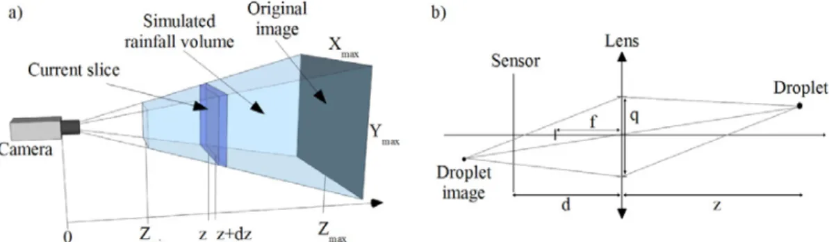
The simulator is based on a camera model associated with a simulated rainfall volume (Fig. 1a). The camera uses a lens and aperture model (Fig. 1b) which makes it possible to simulate the depth of field. The stages of the simulation are explained later in this section.

The simulation algorithm models the rain by layers of rain, from the deepest to the closest (Fig. 1a). Each layer is simulated by randomly drawing drops progressively. The blurring related to the camera setting is then applied by convolution to the entire layer. As the final light intensity of the rain is attached to the value L, the rain transparency factor of each drop is the only parameter remaining to be calculated. The first step is to determine the volume V(z)of rain of the slice of thickness dz at depth z(Fig. 1a). To do this, the camera settings are used to obtain the formula proposed in equation 1. 2 2 ( ) ( ) p dz H W z d f V z d f (1)

The law of Marshall and Palmer (1948) (equation 2) then gives the number of droplets N(a)of each diameter aper unit volume. 0.21 1 1 4 0 0 ( ) a with 4.1 ( in . ) and 0.08 N a N eO Rr mm Rr mm h N cm O (2) Diameteraalso gives the velocity of each droplet from equation 3 provided by Gunn and Kinzer (1949):

3 1.31

3.45.10 1

( ) 9.40 (1 a ) with in and in .

v a e a mm v m s

₍₃₎

Fig. 2 a) Each pixel is covered by the droplet for a limited period as compared with the total exposure time. b) If the droplet does not fully cover a pixel, part of the scene is visible, thereby producing a transparency factor during integration.

For each given diameter a, all the droplets in the slice are then randomly drawn one by one using a uniform distribution on the position and orientation of the streak. Diameter agives the length l(a)of the streak (equation 4).

( ) ( ) ( ) T v a d f l a p z df (4)

Value Įof the sharp transparency mask of the droplet is given by equation 5.

2 1 . min ;1 .min ;1 ( ) ( ) s t a d f p z d f l a D D D §¨§_¨ ·_¸ ·¸ §_¨ ·_¸ ¨_{© ¹} ¸ _{© ¹} © ¹ (5)

This value Įincludes a time factor Įtand an area factor Įs. The time factor corresponds to the case where the

droplet covers a pixel only for part of the total exposure time (Fig. 2.a). The area factor makes it possible to take into account cases where the droplet is too small to cover an entire pixel (Fig. 2.b). The transparency mask of the droplet

MG(of the same size as the input image) is equal to Įwhere the droplet masks pixels and 0elsewhere (equation 6).

, if the droplet masks the pixel ( , ) ( , ) 0, elsewhere G i j M i j _®­D ¯ (6)

According to equation 7, this transparency mask is then added term for term to the transparency mask of the previous drops Mof the slice.

G

M M M (7)

When the drawing of droplets of all sizes of the slice at depth zhas been completed, the sharp transparency mask

Mof the rain at depth zis obtained. This mask is then convoluted by the circle of confusionKerCat depth zto obtain

the blurring associated with the depth of field. Diameter Cof the circle of confusion is given by equation 8. Its intensity is uniform and its integral is equal to 1by conservation of the light energy received by the sensor.

1 ( ) 1 ( ) ( ) ( ) ( ) d z f f d z f C z q z d f N z d f (8) flou M C M Ker (9)

After the convolution given by equation 9, the blurred image of rain transparency at depth zis available. The latter is used to simulate the effect of the rain slice at depth zby following equation 10.

>

@

1 0 1 max

(1- ) with without rain and with the effect of rain on ;

i flou flou i i

I L M M uI I I z Z (10)

Starting with I0the initial image without rain, the final image with digitally simulated rainfall is obtained by

successive additions of rain slices, from the one furthest from the camera to the nearest.

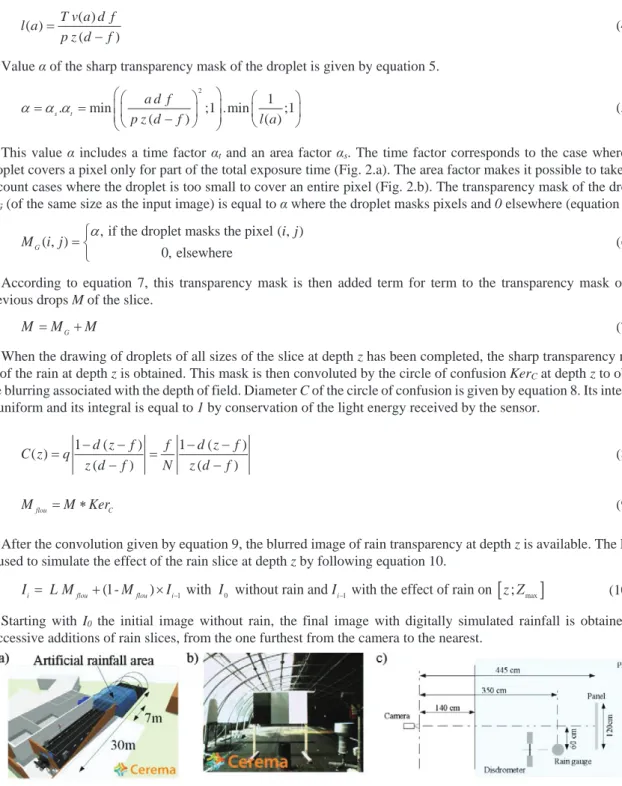
Fig. 3. a) 3D view of the Cerema R&D Fog and Rain platform. b) Example of an image acquired by the camera used for the tests (setting 1, without rain). c) Map of the position of the different elements during acquisitions.

3. Image acquisition protocol in artificial rain

3.1. The Cerema R&D Fog and Rain platform

To test the simulator, the images created by it were compared to images acquired in the Cerema R&D Fog and Rain platform in Clermont-Ferrand (France), Colomb et al. (2008). By projecting water droplets, this platform can simulate different intensities of rainfall. A volume of rain of7 min depth was produced over the 30 mthat the platform provides (Fig. 3a).

3.2. Image acquisition protocol

Several cameras were placed in front of a panel with three uniform colours (Fig. 3b). The cameras were positioned 1.40 mfrom the volume of rain and 4.45 mfrom the panel (Fig. 3c). Two different rainfall rates were used for the validation presented below. Two rainfall sensors using different technologies made it possible to measure the rainfall rate during the acquisitions: a OTT Parsivel disdrometer and a LSI rain gauge. The two sensors were used to determine the average rainfall rate for the two cases shown in the following (111 mm.h-1 _and

64 mm.h-1_{) (table 1).}

Five different cameras (resolution, lens, settings, etc.) were used to acquire the images. Only the images from the Allied Vision Technologies Marlin F033C camera were analysed here. In order to validate the simulator with different settings, two extreme camera settings were used for the aperture (N) and the exposure time (T). The other camera settings remained fixed: the focal length (f = 8 mm), the distance where the plan of focus is made (d = 6 m), and the size of a pixel (p = 9.9 µm). The two extreme settings and both rainfall rates made it possible to obtain four different tests (table 1). Fig. 4 shows extracts of images obtained .

Table 1. The four tests set up to validate the simulator. Tests Rainfall rate Camera setting Test 1 111 mm.h-1

Setting 1 (N = 1.4, T = 0.032 ms) Test 2 64 mm.h-1 _{Setting 1 (N = 1.4, T = 0.032 ms)} Test 3 111 mm.h-1 _{Setting 2 (N = 16, T = 0.03 s)} Test 4 64 mm.h-1 _{Setting 2 (N = 16, T = 0.03 s)}

3.3. Image acquisition protocol in natural rain

The same weather sensors and the same cameras were placed outdoor according to the same protocol. Automatic image acquisition software was developed to obtain images in natural rain. The weather conditions did not, however, allow enough data to be obtained at the time of publication. These data will be analysed using the same protocol and presented in a future publication.

Fig. 4. Extracts of images for setting 2 of the camera. a) Artificial rain (111 mm.h-1

). b) Simulated rain (110 mm.h-1

4. Validation of the images produced by the simulator according to two methods

4.1. Evaluation method using standard deviation

The images produced digitally by the rainfall simulator follow the physical parameters of the rain and the camera. These images must therefore be evaluated quantitatively against images of real rain.

The first evaluation method proposed makes use of the work presented in Garg and Nayar (2007). This method is based on measuring the standard deviation over a homogeneous image area. The intensity of a pixel fluctuates when a raindrop passes over it between the value of the scene without rain and the value of raindrops (Fig. 5a).

From this observation, Garg and Nayar (2007) shows that the standard deviation of a small volume of rain may be connected to the rainfall rate and camera settings. Measurement of the standard deviation over an area where the scene is homogeneous is therefore a first method for validating digitally simulated images.

For each image, the standard deviation is measured over a uniform region of interest. N×Mpatches of L×K (15×30)

pixels and spaced out by 2pixels are then extracted (Fig. 5b). For each patch, the standard deviation of the intensity is calculated by following equation 11. Then, the average of the standard deviations of all the image patches is then calculated (Fig. 5.b.). Measurement Mıbased on the standard deviation is obtained in this way.

In the case of an image without rain, the scene and the camera being fixed, only the noise of the camera is measured by Mıwhich is then very low. Conversely, when there is rain, some pixels will be covered by the rain, while others

will not. Measurement Mıwill then depend on the rainfall rate and the camera settings. 4.2. Evaluation method using ZNCC

The second evaluation method is based on Zero-Mean Normalized Cross Correlation (ZNCC). The distribution of the ZNCC between pairs of random patches from a natural image (Fig. 6a) has a strong peak at 0, Chen and Hsu (2013). This peak originates from patches that are non-discriminating.

When rain is present on the image, the latter provides an additional noise. Adding this noise decreases the number of non-discriminating pairs of patches, especially since this noise is well correlated throughout the image. The peak on the distribution of the ZNCC is therefore greatly reduced when rain is present.

The evaluation measurement based on the ZNCC is as follows (Fig. 6b). For each image, 50,000pairs of patches measuring 11×11pixels are drawn from the image using uniform distribution. The ZNCC between the two patches is calculated by following equation 12. The histogram of the ZNCC(histZNCC) is then updated for the pair of patches

under consideration. When all pairs have been processed, the histogram is then normalized (integral equal to 1).

Fig. 6 a) Example of a histogram on the ZNCC(histZNCC) for a natural image. b) Diagram explaining measurement MZNCC.

In order to get back to a single value to be able to process a series of images, a measurement MZNCCbased on an

integration is proposed in equation 13. The interval [-0.03 ; 0.03] enables the peak to be framed with sufficient accuracy to measure the evolution of the histogram. This measurement MZNCChas the same direction of variation as

measurement Mıwith respect to the rainfall rate.

0.03 0.03 1 ZNCC( ) ZNCC his x M _³ t dx (13) 4.3. Results

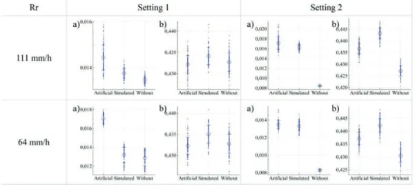
The protocol described in section 3.2 was used to acquire four image sets with different experimental conditions. The simulator is validated using three images: an image without rain, an image with artificial rain, and an image of the simulated rain. To obtain statistically reliable results100images sets were used. Fig. 7 shows the results for the two settings and two rainfall rates tested. The metric based on the standard deviation (or ZNCC, respectively) is presented in a (or b respectively). Overall, variations in metrics for simulated rain and artificial rain are consistent. The two measurements increase in the presence of artificial rain or when digitally simulated rainfall is added.

However, this change in measurements for artificial rain is not significant for camera setting 1. This setting corresponds to an infinite depth of field with a small aperture and a long exposure time. These parameters are those for which the rain has the least impact on the images Garg and Nayar (2007). This result is consistent but shows that the proposed measurements not permit to conclude that the simulator is valid for all camera settings. Conversely, for setting 2, when the aperture is large and the exposure time short, the effect of the artificial rain is significant for both measurements and both rainfall rates. This is also in keeping with the proposals made by Garg and Nayar (2007).

The results obtained for the rain simulator are also consistent. As far as setting 1 is concerned, the variations in both measurements proposed and for both rainfall rates are not significant, as for artificial rain. In the case of setting 2, which is the one that most highlights the rain, the measurement based on the standard deviation validates the impact of simulated rain as compared with artificial rain. The values of this measurement are indeed very close and they are significantly distant from the measurement for images without rain, for both rain intensities tested. For the measurement based on the ZNCC, the impact of simulated rain turns out to be greater than that of artificial rainfall for both rainfall rates. This impact still remains consistent since the measurement increases.

To conclude, although the two proposed metrics (based on standard deviation and based on the ZNCC) do not make it possible to measure the impact of the rain for certain camera settings (setting 1), the validity of the simulator has been shown for these metrics in the case of camera setting 2. This setting is the one that most highlights the rain.

5. Test methodology for an image feature

5.1. Objective of validating features in adverse weather conditions

In the road environment, features are used in a number of applications both on infrastructure and in vehicles. On infrastructure, for example, they are used in pedestrian detection Viola et al. (2003), Zhao et al. (2008), or vehicle detection Tan and Baker (2000), Cucchiara et al. (2000), algorithms. On board vehicles, they are used for pedestrian detection, Ess et al. (2009), Bertozzi et al. (2007), vehicle detection Leibe et al. (2007), Franke et al. (2013), lane detection Lee and Cho (2010), Jung and Kelber (2005), visual odometry, Royer et al. (2007), or traffic sign detection García-Garrido et al. (2011), Ruta et al. (2011). These image features are commonly used; they are tested on many databases. However, most databases are composed of images acquired in favourable weather conditions. Adverse weather conditions such as fog, rain or snow are not considered in the literature for the evaluation of these features. The rain simulator can help to begin to answer the question of the validity of these features, which are essential for algorithms, in rainy conditions. To do this, a method for evaluating the robustness of the features in rainy conditions has been established, based on the images obtained by the simulator. This method is described in the next section. 5.2. Method for evaluating the robustness of features in rainy conditions

To evaluate the robustness of features in rainy conditions the following protocol is proposed. An image set without rain is acquired by a camera. These images are used to create images for different rainfall rates by means of the digital simulator presented and validated previously. The camera settings entered into the simulator are the same as those used for acquisition. The image feature to be analysed is then applied to the image set without rain and to image sets with at different rainfall rates. For each set of different rainfall rates, the similarity between the initial image feature and the image feature with rain is measured. For each rainfall rate, a set of similarity measurement points of the same cardinality as the number of images in each set is thereby obtained. This set, of100 images here, reduces the measurement uncertainty.

The similarity measurement is calculated a second time between the original image and another image without rain. This second image without rain is drawn randomly. This second measure provides a standard value for the camera. It corresponds to the noise of the camera during acquisition.

As shown in equation 14, the similarity measure adopted (SimL2) is the inverse of norm L2between the two images.

Norm L2 is reversed so that the similarity measure increases when two images are alike.

5.3. Test of the method for evaluating robustness in rainy conditions on a well-known feature

The method for assessing the robustness of image features in rainy conditions is now applied to the feature of Harris and Stephens (1988). The Harris feature was chosen because it is a well-known feature which is used in many applications in image processing and analysis. Although it is also used outside the road context, it is included, in this context, in vehicle detection Leibe et al. (2007), pedestrian detection Ess et al. (2009) or visual odometry algorithms

Royer et al. (2007). This feature is in principle used as an interest point detector. It sends high values into corners or into easily identifiable areas in contrast to uniform areas for example. The way it operates and its use in the algorithms are not described here. Only its robustness in rainy conditions was evaluated. The implementation of the OpenCV Harris feature was used for these tests. The images were acquired using camera setting 2. This setting was validated in section 4.3.

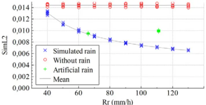
The results of this test (Fig. 8) show that the similarity measurement drops when the rainfall rate increases. The similarity measure of the standard without rain is not infinite and is constant because it corresponds to noise induced by the camera. For40 mm.h-1_{, the similarity measurement is nearly identical with and without rain. For a lower rainfall}

rate, rain has no more impact on the robustness of the Harris feature than the noise of the camera. However, when the rainfall rate reaches a value of 130 mm.h-1_{, the similarity measurement decreases by half as compared to the standard}

without rain. The Harris feature is then strongly impacted by the rain.

Finally, the values of the similarity measurement for the data acquired in artificial rain (at 111 mm.h-1_{and 64 mm.h} -1_{) are quite close to those obtained for simulated rain. This result is therefore in keeping with that obtained during}

validation of the simulator.

6. Conclusion

A digital rain simulator model was proposed. Two methods of validating the simulator involving comparing the images obtained by the latter with images acquired in artificial rain were then implemented. These have shown that the simulator obtained lifelike images for certain camera settings. Validation methods did not, however, enable any conclusions to be drawn for extreme camera settings where rain has a very low impact on the images.

The simulator was then used to implement a method for evaluating the robustness of image features in rainy conditions. This evaluation showed that the Harris feature undergoes a deterioration when the rainfall rate increases.

These first results are therefore encouraging but still require more in-depth study. The range of acceptable settings for the simulator validation method will have to be evaluated. Similarly, although the method for assessing the robustness of the features was used to measure a deterioration in the Harris feature, the limit at which this deterioration becomes too great for the algorithms to operate properly remains unknown. Work on the final functions could therefore be set up. In addition, this robustness evaluation method will have to be tested on other conventional features. When the database of images acquired in natural rain conditions is available, new evaluations of features can be made with the same protocol. These tests under real conditions, although less extensive, will then be of an even greater validity.

Fig. 8. Results of the feature analysis method for the Harris feature. The camera settings correspond to setting 2 mentioned above.

Finally, despite the lack of completeness of the results presented, they have made it possible to present and validate a comprehensive evaluation method of the robustness of image features in rainy conditions. These conditions appear to have a great impact on the first example. This therefore fully justifies the need to take into account adverse weather conditions for computer vision in the road environment. The development of intelligent transport systems (ITS) is expanding and uses this type of image processing tool extensively. These tools must therefore have minimal error rates and cannot afford to ignore validation in all conditions encountered, particularly in varying weather conditions.

Acknowledgements

The authors would like to thank LabEx ImobS3 and ViaMeca innovation cluster thanks to which relations between the Clermont-Ferrand laboratories are even stronger. They would also like to thank the whole team in charge of the Cerema R&D Fog and Rain platform.

References

Bertozzi, M., Broggi, a., Rose, M.D., Felisa, M., Rakotomamonjy, a., Suard, F., 2007. A Pedestrian Detector Using Histograms of Oriented Gradients and a Support Vector Machine Classifier. 2007 IEEE Intell. Transp. Syst. Conf. 143–148. doi:10.1109/ITSC.2007.4357692 Chen, Y., Hsu, C., 2013. A Generalized Low-Rank Appearance Model for Spatio-temporally Correlated Rain Streaks. ICCV 2013 IEEE. Colomb, M., Hirech, K., André, P., Boreux, J.J., Lacôte, P., Dufour, J., 2008. An innovative artificial fog production device improved in the

European project “FOG.” Atmospheric Res. 87, 242–251. doi:10.1016/j.atmosres.2007.11.021

Cucchiara, R., Piccardi, M., Mello, P., 2000. Image analysis and rule-based reasoning for a traffic monitoring system. Syst. IEEE Trans. Ess, A., Leibe, B., Schindler, K., Van Gool, L., 2009. Robust multiperson tracking from a mobile platform. Pattern Anal. Mach. Intell. 31, 1–14. Feng, Z., Tang, M., Dong, J., Chou, S., 2006. Real-time rain simulation. Comput. Support. Coop.

Franke, U., Pfeiffer, D., Rabe, C., Knoeppel, C., Enzweiler, M., Stein, F., Herrtwich, R.G., 2013. Making bertha see. Proc. IEEE Int. Conf. Comput. Vis. 214–221. doi:10.1109/ICCVW.2013.36

García-Garrido, M. a., Ocaña, M., Llorca, D.F., Sotelo, M. a., Arroyo, E., Llamazares, a., 2011. Robust traffic signs detection by means of vision and V2I communications. IEEE Conf. Intell. Transp. Syst. Proc. ITSC 1003–1008. doi:10.1109/ITSC.2011.6082844

Garg, K., Nayar, S.K., 2007. Vision and Rain. Int. J. Comput. Vis. 75, 3–27. doi:10.1007/s11263-006-0028-6 Garg, K., Nayar, S.K., 2003. Photometric Model of a Rain Drop. Rain.

Gunn, R., Kinzer, G., 1949. The terminal velocity of fall for water droplets in stagnant air. J. Meteorol. Harris, C., Stephens, M., 1988. A combined corner and edge detector. Alvey Vis. Conf.

Jung, C.R., Kelber, C.R., 2005. A lane departure warning system using lateral offset with uncalibrated camera, in: IEEE Conference on Intelligent Transportation Systems, Proceedings, ITSC. pp. 348–353. doi:10.1109/ITSC.2005.1520073

Lee, J., Cho, J., 2010. Effective lane detection and tracking method using statistical modeling of color and lane edge-orientation.

Leibe, B., Cornelis, N., Cornelis, K., Gool, L.V., 2007. Dynamic 3D Scene Analysis from a Moving Vehicle. Proc. IEEE Comput. Soc. Conf. Comput. Vis. Pattern Recognit. CVPR 1–8. doi:10.1109/CVPR.2007.383146

López, C.C., 2011. Real-time Realistic Rain Rendering.

Manning, R., 1993. Stochastic Electromagnetic Image Propagation Through the Atmosphere. McGraw-Hill, Inc. Marshall, J., Palmer, W., 1948. The distribution of raindrops with size. J. Meteorol.

Potmesil, M., Chakravarty, I., 1982. Synthetic image generation with a lens and aperture camera model. ACM Trans. Graph. TOG.

Rousseau, P., Jolivet, V., Ghazanfarpour, D., 2006. Realistic real-time rain rendering. Comput. Graph. Pergamon 30, 507–518. doi:10.1016/j.cag.2006.03.013

Royer, E., Lhuillier, M., Dhome, M., Lavest, J.-M., 2007. Monocular Vision for Mobile Robot Localization and Autonomous Navigation. Int. J. Comput. Vis. 74, 237–260. doi:10.1007/s11263-006-0023-y

Ruta, A., Porikli, F., Watanabe, S., Li, Y., 2011. In-vehicle camera traffic sign detection and recognition. Mach. Vis. Appl. 22, 359–375. doi:10.1007/s00138-009-0231-x

Starik, S., Werman, M., 2003. Simulation of rain in videos. Texture Workshop ICCV.

Tan, T.N., Baker, K., 2000. Efficient image gradient based vehicle localization. IEEE Trans. Image Process. Publ. IEEE Signal Process. Soc. 9, 1343–56. doi:10.1109/83.855430

Viola, P., Jones, M., Snow, D., 2003. Detecting pedestrians using patterns of motion and appearance. Comput. Vis. 2003. Wang, L., Lin, Z., Fang, T., Yang, X., 2006. Real-time rendering of realistic rain. ACM SIGGRAPH 2006.

Wang, T., Clifford, S.F., 1975. Use of rainfall-induced optical scintillations to measure path-averaged rain parameters. J Opt Soc Am 65, 927–937. doi:10.1364/JOSA.65.000927

Zhao, T., Nevatia, R., Wu, B., 2008. Segmentation and tracking of multiple humans in crowded environments. IEEE Trans. Pattern Anal. Mach. Intell. 30, 1198–1211. doi:10.1109/TPAMI.2007.70770