Forecasting
Daniel Waller
Submitted for the degree of Doctor of
Philosophy at Lancaster University.
Retail forecasting is a diverse and dynamic research area encompassing a variety of different topics. The advent of online channels, the increasing complexity of product ranges, and the shortening lifespan of many items are as examples of some of the new challenges that maintain the importance of improving forecasting in this domain. This thesis aims to address questions in retail forecasting that are closely linked with relevant problems faced in the industry. As such, the problems have been identified through a combination of reviewing the academic literature, discussion, and engage-ment with practitioners.
This thesis starts by considering the situation where demand series are influenced by multiple seasonal and calendar effects. This is a challenge which is widespread due to high frequency sampling and decision making in retailing. We develop a new model to accommodate flexibility in modelling complex seasonal patterns, which also aids with mitigating the effect of short demand histories on forecasting performance. The new model is embedded in an innovations state-space formulation and it is demon-strated empirically using wholesale food data to provide competitive forecasting ac-curacy to established benchmarks.
Next, the dual problems of SKU-level model parameter estimation and forecast-ing are considered. For retailers experiencforecast-ing frequent promotional activities, this is a principal issue. The parameter estimates provide insights about the elasticity of different factors on demand for the SKU, and therefore inform marketing planning. Accurate forecasts, for both promotional and baseline periods, support other func-tions such as replenishment and inventory management. First, a geometric parameter inheritance procedure is proposed, which uses aggregate information within a prod-uct hierarchy to improve parameter estimates under certain assumptions. At brand level, it is typically easier to better estimate elasticity effects, making this strategy preferable. Second, a debiasing approximation is derived for the forecasting proce-dure, which is demonstrated to reduce bias, whilst remaining competitive in terms of forecast accuracy, as shown in a simulation study. The debiasing approximation is then evaluated with an inventory simulation study, which examines the conditions under which improvements in inventory performance can be gained. The conclusions give useful insights for inventory managers, and demonstrate that bias is a significant factor in inventory performance.
Firstly, I gratefully acknowledge the financial support of the EPSRC, through the STOR-i Centre for Doctoral Training, and of Aimia, in co-sponsoring this work. I’d like to thank all those at Aimia that have helped shape this research.
I’d like to thank the directors of STOR-i, and the administrative staff, along with anyone else who has been involved in running the centre, for their tireless efforts behind the scenes in making STOR-i what it is. It’s hard to imagine a better place to do a PhD. I would also like to thank everyone in the community of STOR-i students that has come and gone during my time here for your friendship. The people at STOR-i really are the best there are.
I would like to give great thanks to both of my supervisors, John Boylan and Nikolaos Kourentzes, for all the time and effort they have spent to guide me in this project. It would have been simply impossible without their consistent, invaluable advice, patience and encouragement. I also thank the members, past and present, of the Centre for Forecasting, who have always been generous in sharing their knowledge. Last but not least, I would like to thank my family, and my girlfriend Anne, for their love and support throughout this time.
I declare that the work in this thesis has been done by myself and has not been submitted elsewhere for the award of any other degree.
Daniel Waller
Abstract I
Acknowledgements III
Declaration IV
Contents VIII
List of Figures XI
List of Tables XIII
1 Introduction 1
2 Multiple seasonality in retail 7
2.1 Introduction . . . 8
2.2 Literature review . . . 10
2.2.1 Types of seasonality . . . 10
2.2.2 Multiple seasonality . . . 11
2.2.3 Exponential smoothing based methods . . . 14
2.3 A mixed-representation parsimonious seasonal model . . . 24
2.3.1 Innovations state-space model . . . 26
2.3.2 Estimation . . . 29 2.3.3 Model specification . . . 30 2.4 Empirical evaluation . . . 31 2.4.1 Dataset . . . 31 2.4.2 Methods . . . 32 2.4.3 Error measures . . . 33 2.4.4 Results . . . 34 2.5 Conclusions . . . 39
3 Sources of bias in loglinear models for retail 42 3.1 Introduction . . . 43
3.2 Literature review . . . 45
3.2.1 Sales response models . . . 45
3.2.2 Aggregation in retail modelling . . . 46
3.2.3 Bias in loglinear models . . . 51
3.3 Geometric parameter inheritance . . . 52
3.4 Bias in loglinear models . . . 55
3.4.1 Bias quantification . . . 55
3.4.2 Correction approximations . . . 59
3.4.3 Combination of parameter inheritance and bias approximations 60 3.5 Simulations . . . 61
3.5.1 GPI simulations . . . 61
3.5.2 Forecast approximation simulations . . . 66
3.5.3 Combined simulations . . . 74
3.6 Conclusions . . . 77
4 The inventory performance of bias-corrected sales forecasts 79 4.1 Introduction . . . 80
4.2 Methods . . . 83
4.2.1 Sales model . . . 83
4.2.2 Forecasting methods . . . 84
4.3 Inventory setup . . . 86
4.3.1 Type of inventory process . . . 86
4.3.2 Service target and calculation of safety stock . . . 87
4.4 Simulation setup and results . . . 90
4.5 Results . . . 95
4.5.1 Safety stock calculation method . . . 95
4.5.2 Varying parameter combinations . . . 98
4.5.3 Tradeoff between service level difference and average OHI . . . 103
4.5.4 Connection with forecast bias/variance . . . 106
4.6 Conclusions . . . 111
5 Outcomes and further work 117 5.1 Thesis summary . . . 117
5.3 Future directions . . . 122
A Multiple seasonality in retail - appendices 126
A.1 Model specification for PES . . . 126 A.2 Multiplicative PES . . . 129 A.3 MAPE results . . . 130
B The inventory performance of bias-corrected sales forecasts -
ap-pendix 134
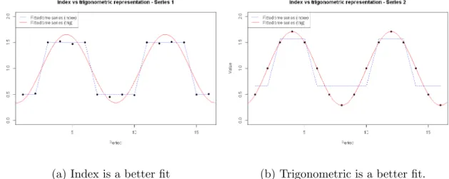
2.3.1 An illustration that both the trigonometric and index representations of seasonality can fit better to different series. . . 25
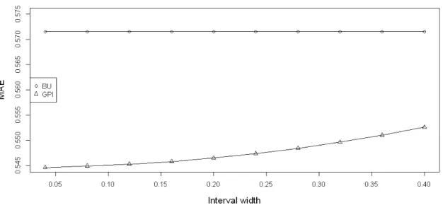
3.5.1 Lineplot showing the MAE of parameter estimates as the sampling interval widens. . . 65 3.5.2 Surface plots showing the ratio of MAE between different forecasting
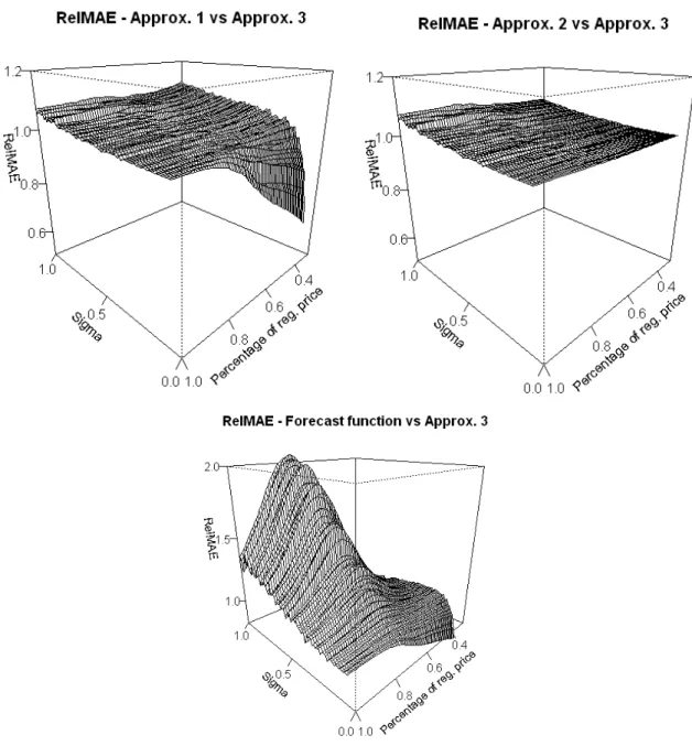
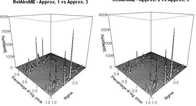
functions, using Approximation 3 as the benchmark, varying over price cuts and variance. From top (i) Approximation 1 (ii) Approximation 2 (iii) Base forecast function. The geometric means of the RelMAE surfaces are: (i) 1.019 (ii) 1.018 (iii) 1.198 respectively. . . 68 3.5.3 Surface plots showing RelAbsME between different forecasting
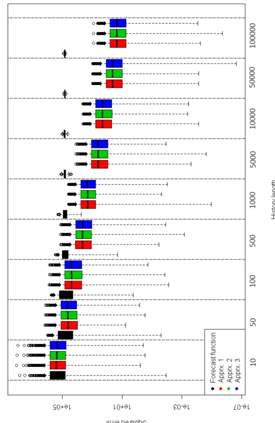
func-tions, using Approximation 3 as the benchmark, varying over price cuts and variance. From top (i) Approximation 1 (ii) Approximation 2 (iii) Base forecast function. The geometric means of the surfaces are (i) 1.039 (ii) 1.042 (iii) 7.534 respectively. . . 69 3.5.4 Boxplots showing the distribution of squared forecast errors when P =
0.5 for varying history lengths. . . 71
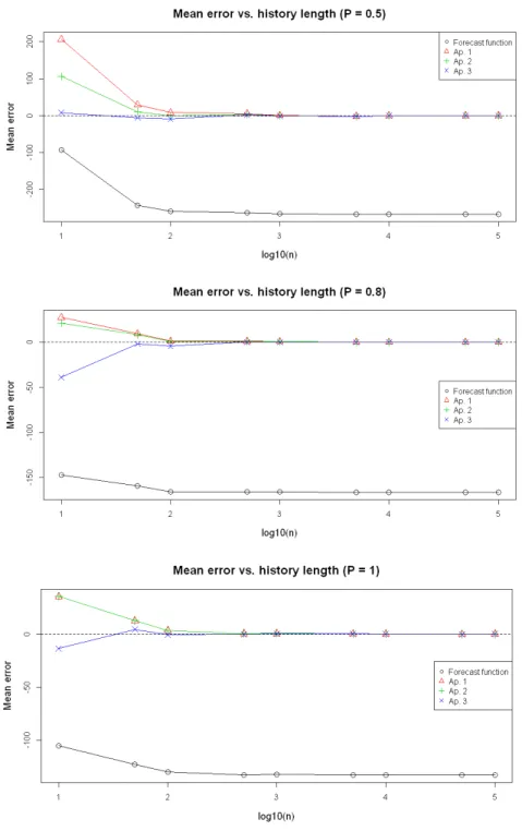
3.5.5 Line plots showing the mean error of each of the three approximations and the forecast function, compared to the theoretical average, varying over length of data history. From top (i) Price 1
2 of regular price (ii)
Price 45 of regular price (iii) Full regular price. . . 72
4.5.1 Aggregate performance over all 243 parameter sets of the 9 forecast method/safety stock calculation method combination. . . 97 4.5.2 Lineplots illustrating the performance in terms of (i) CSL, and (ii)
Av-erage OHI, as history length varies of the forecasting methods. Results here are for a 95% target CSL. . . 101 4.5.3 Tradeoff between achieved service level and average OHI. The
param-eter set is β = −2, σ = 0.5, promotional frequency = 0.1 and history length = 20. . . 104 4.5.4 Scatterplot displaying relative av. OHI vs. service level difference for
all parameter combinations. . . 105 4.5.5 Forecast bias vs. (i) RelAvOHI (ii) Service level difference, for all
parameter combinations. . . 112 4.5.6 Forecast variance vs. (i) RelAvOHI (ii) Service level difference, for all
parameter combinations. . . 113 4.5.7 Forecast accuracy vs. (i) RelAvOHI (ii) Service level difference, for all
parameter combinations. . . 114
A.1.1Daily sales to the education sector. . . 127 A.1.2Daily sales to the education sector during the 6 weeks of summer holidays.129
A.3.1Beanplot showing the one-step-ahead percentage forecast error distri-bution on the first series, for 3 selected methods. . . 132
2.4.1 Benchmark methods . . . 33
2.4.2 AvgRelMAE figures, individual horizons. . . 35
2.4.3 AvgRelMAE figures, cumulative horizons. . . 37
2.4.4 AvgRelMAE figures, 1-7 day cumulative horizon, special days vs. no special days. . . 39
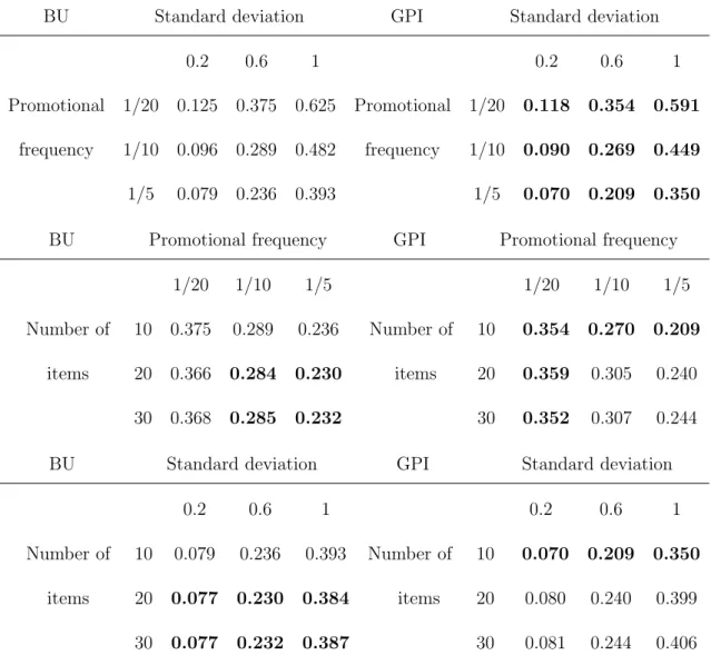
3.5.1 Parameter MAE figures for the BU and GPI methods under varying standard deviation, price cut frequency and number of items in the group. . . 63
3.5.2 Ratios of MSE and components as standard deviation varies. . . 75
3.5.3 Ratios of MSE and components as history length varies. . . 76
4.3.1 Choices for the components of the inventory system . . . 90 4.4.1 Showing the four different dimensions across which we vary parameters
in the simulation study. The origin represents the parameter combi-nation sitting in the middle of the range in each direction, whilst the other rows show the higher and lower alternatives for each dimension 92
4.5.1 Service level difference and relative average OHI simulation results for
Miller and EBC under varying conditions. . . 98
4.5.2 Bias/RMSE/variance ratio of EBC approx. to Miller approx., alongside percentage inventory saved and service level lost. . . 109
5.2.1 Summary of managerial implications. . . 121
A.3.1MAPE figures, individual horizons. . . 131
Introduction
The quality of retail forecasting has been widely demonstrated to have a significant impact on retailers’ performance. Both academic researchers and forecasting practi-tioners have directed a lot of attention to improving and developing forecasting models for many years (Fildes et al., 2019); it continues to be a crucial research focus, con-sidering the changing environment in the industry today. In a recent article, Seaman (2018) presents some of the considerations that retail forecasters should take into ac-count and how forecasts can be used differently, depending on the objectives. One of the important challenges touched upon is forecasting for highly seasonal and pro-motional items, particularly around the holiday period. Commenting on this article, Boylan (2018) provides more background on recent trends. A surge in competition, as well as changes in the mix of store types and a shift towards offering more diverse product ranges have all pushed retailers towards data analytics as a means to gain an advantage over rival firms. Boylan (2018) also cites how shorter supplier lead times have led to retail data being captured in shorter time buckets than ever before.
This increased granularity of data has revealed seasonal patterns that were previously unobservable due to their high frequency, leading directly to a growing importance of modelling complex seasonality. Furthermore, a proliferation of data, partly influ-enced by the rise of loyalty programmes, has placed an emphasis back on extracting signals from noisy, disaggregate information. The dual problems of parameter esti-mation and forecasting are important challenges for this data type, particularly in the context of promotional modelling; they influence many retail functions, including inventory replenishment and promotional strategy.
In this thesis, we are motivated to provide solutions to real issues in retail forecast-ing that are faced by practitioners. In particular, part of the motivation for the thesis is from co-sponsorship by Aimia, a loyalty analytics company. In dealing with retail data from a wide range of different sources, the company is well-placed to recognise the problems that are faced within the sector, and many of the problems that moti-vate this research have come from discussions with them and other practitioners in the area. Additionally, real-world data that has been shared by the company have been invaluable in helping to provide both intuition and motivation for the work. Chap-ter 2 sees the most direct example of this, where various methods for multi-seasonal forecasting are applied on one of these datasets in an empirical study; nonetheless, insights gained from the real datasets have influenced all chapters. Meanwhile, this work has also aimed to contribute to various different areas in the academic literature. As the contents and structure of the thesis is laid out in the following paragraphs, we try to describe the process by which a practical problem was taken as motivation and then abstracted into a research question that addresses gaps in the academic
literature in each case.
In Chapter 2, the motivation to study the issue of multiple seasonality was formed through both an appraisal of demand series from real retail datasets from varying sources, and also through conversations with forecasting practitioners, who identified the interaction between special events and other more regular calendar-based season-alities as a difficult phenomenon to forecast. To examine this issue in an academic setting, the general methodology of dealing with seasonalities in time series forecast-ing was reviewed. It was found that, whilst recent work (eg. Taylor and Snyder, 2012; De Livera et al., 2011) proposed methods to reduce the number of parameters need-ing to be estimated, no approach specifically accounted for the short demand histories typical of retail, whilst still accommodating flexible modelling of seasonalities and the interaction between them. A new model is developed, the mixed parsimonious model, which addresses this problem, and an empirical evaluation, carried out on real-world data from a food wholesaler, yields promising results for the proposed model.
Having overcome modelling challenges associated with multiple seasonal periodic-ities in retail data, the focus turns to modelling promotional events, which is another major complication for forecasting in the sector. In Chapter 3, the initial problem identified is the estimation of the typically-seen-in-practice loglinear regression-model parameters, for forecasting at the stock keeping unit (SKU) level. This is a problem for practitioners because SKU-level data series often have short histories and are very noisy, resulting in parameter estimates that are inaccurate, which has knock-on effects for both forecasting and other analytics carried out by the retailer; alternatively, in-sights into products can be gained by clustering SKUs within a subcategory eg. brand
or target market. By contrast, parameter estimation and forecasting at higher levels of the retail hierarchy is much easier; thus, we are motivated to explore using hierar-chical information at higher levels of aggregation to alleviate problems at lower levels. We found that potential gaps existed to exploit the abundance of SKU-level data available in recent times to better use hierarchical information, with much research taking place before such data was available (eg. Christen et al., 1997). Furthermore, the bias in the forecasting procedure had not been fully explored eg. Miller (1984). Two methodological developments were made: (i) a geometric parameter inheritance scheme to estimate a common parameter at an aggregate level without incurring bias, and (ii) a forecast debiasing approximation which corrects for bias incurred in the parameter estimation process. The performance of both of these developments, along with the combination of the two, is examined through a simulation study.
In Chapter 4, the impact of the forecast approximation developed in the previous chapter on inventory management is examined. Linking improvements in forecasting procedure through to their consequences in stock and service levels is important for practitioners (Gardner, 1990); inventory performance metrics are often much closer to the real factors that influence operational decisions than more abstract forecast accuracy measures (Kourentzes, 2013). We found this relationship to be important, and underdiscussed in the academic literature despite the earlier references. Fur-thermore, issues around bridging promotional modelling and inventory management, such as calculating safety stock for promotional periods, are also gaps needing further research. This chapter contains details of a simulation study, which demonstrates the performance of our approach under a variety of conditions. We also examine the
relationship between different properties of the forecasts, such as bias, accuracy and variance, and dimensions of inventory performance such as average on-hand inventory and service level, to further understand the drivers of inventory performance.
We summarise the findings of the thesis in Chapter 5, outlining the main contri-butions that have been made. The implications for practitioners are discussed, along with comments on the limitations of the work, and then we expand on some possible directions for future research.
Before presenting the main body of the thesis, we summarise the contributions. The first contribution is a new method for modelling complex seasonal patterns, em-bedded in an innovations state-space model. The new method is found through an empirical study to improve forecasting accuracy over existing methods in all periods, including where calendar effects are present, and for cumulative forecast horizons. The second contribution is a geometric parameter inheritance scheme for estimating SKU-level parameters, which avoids bias normally present when estimating param-eters at a higher aggregation level. The procedure is examined through simulations and found to improve the accuracy of parameter estimates over individual estima-tion, under the assumption that the SKUs share a parameter in common. Third, an approximation for debiasing forecasts is derived and found through simulations to significantly reduce bias, whilst yielding similar accuracy compared with existing forecast approximations. A combined method implementing geometric parameter in-heritance and the debiasing approximation is also demonstrated to reduce bias in the forecasts in return for a modest increase in forecast mean squared error. Lastly, the debiasing approximation is shown through simulations to reduce holding costs, albeit
at expense of a slightly reduced service level, in an inventory management system. Examining the forecast properties in terms of bias, accuracy and variance, the situa-tions in which stock holding costs are decreased the most are found to be somewhat associated with those where the bias is reduced most.
Multiple seasonality in retail
Abstract
In retailing, there are often time series where the value in a period is influ-enced by more than one seasonal effect. A typical example is that of a daily time series of sales, fluctuating due to both the weekly and annual patterns, in addition to any calendar effects. These complex seasonal patterns are more common with the increasing granularity of data, and present a challenge to forecast. In this paper, we examine how multiple seasonal forecasting meth-ods mainly originating from the short-term energy forecasting literature, can be implemented in the retail domain. The features of retail data are discussed, and short data histories are found to be particularly problematic for existing forecasting methods. To address this issue, a novel approach is developed for modelling multiple seasonality. The new method, embedded in an innovations state-space framework, is based on mixing two alternative representations of seasonality to make best use of the limited data. It is tested against current methods in an empirical study, using data from the food wholesale sector, and
the results show that our approach outperforms other methods in most cases. We discuss reasons behind the observed improvements, and suggest how the logic behind our model might be extended to a more general setting.
2.1
Introduction
Seasonal variation in time series is a common and wide-ranging phenomenon which has been extensively studied in many guises. Exponential smoothing forecasting mod-els have treated times series as a composition of three components: trend, seasonality and error (Hyndman et al., 2008); these models are studied and adapted to cope with new challenges in measuring seasonal demand in retail by using aggregate sales information to estimate seasonal indices (Dekker et al., 2004) or by using regressors for calendar effects to facilitate temporal aggregation (Kourentzes and Petropoulos, 2016). ARIMA models are built by considering autocorrelations, where the seasonal variant contains additional components of this type associated with seasonal differ-ences (Box et al., 2015). Multivariate time series methods, such as regression, often encode seasonality via a set of dummy variables, while machine learning approaches typically follow one of these approaches (Barrow and Kourentzes, 2018). These ap-proaches are widespread in both research and practice.
The seasonality of a series is often defined as a predictable, periodic variation in the series mean (Ord et al., 2017). Implicit in this definition is the idea of a single seasonality, repeating over time. The development of models able to account for multiple seasonalities is much newer (Taylor, 2003).
With the availability of more granular sales data, modelling multiple seasonality and calendar effects is a problem which is becoming more important for the retail sec-tor. Many product sales vary by weekly and annual patterns of seasonality; calendar effects such as Christmas also have a strong influence. Understanding these influ-ences is vital for producing accurate forecasts, and subsequently for making inventory management decisions. (Ramos et al., 2015)
So far in the academic literature, there is a significant gap in the application of multiple seasonal forecasting methods in retailing contexts. The multiple seasonality literature is motivated by applications in sectors such as short-term energy/utility forecasting and call centre forecasting, among others. One of the contributions of this paper is to consider this body of methods in the context of retail, and demonstrate their benefits and drawbacks.
It is obvious that retail forecasting throws up other hurdles that are not present in other domains. One significant issue is that data histories in retail are typically much shorter, often lasting two to three years, or even less; the unavailability of long histories can either be down to a lack of storage capability or the lack of a process to store data for that length of time. This places limitations on the complexity of the model that can be estimated, which in turn limits the applicability of many existing methods. Another issue is the interaction of different seasonal effects; for example, the pattern of spending around Christmas differs according to which day of the week Christmas Day itself falls on. The contribution of this paper is a new model which is an adaptation of previous models to address theses hurdles.
on multi-seasonal forecasting, examining methods from a retail perspective. Section 3 describes the proposed model, which we term themixed parsimonious model. Section 4 sets out two empirical studies, in different areas of retail forecasting, that assess how the methods can be implemented in this setting and assess their performance. Section 5 concludes and hints at future research.
2.2
Literature review
2.2.1
Types of seasonality
We clarify a few definitions related to seasonality for ease of future reading. First, seasonality may be thought of as being either deterministic or stochastic. Determin-istic seasonality is defined as behaviour where the unconditional mean of the process varies throughout the period, but the seasonal profile is stable over time (Ghysels and Osborn, 2001). For instance, a deterministic representation of a series yt might look like: yt = S X s=1 zsδst+εt , (2.2.1)
where zs is the conditional mean for season s, δst are dummy variables and εt is a weakly stationary, zero-mean, IID stochastic process. Stochastic seasonality describes a process where the seasonal shape depends on previous disturbance values, therefore allowing the seasonal profile to vary over time. For example, in a stochastic seasonal AR(1) process, the seasonal indices are defined as:
where t is the current season. Note that the stochastic seasonal process requires s initial seasonal valueszs,0, wheres is the length of the seasonality.
The second dichotomy we present is in the representation of deterministic sea-sonality; both a dummy variable representation and trigonometric representation are possible. The dummy variable representation is shown in (2.2.1); the trigonometric one is yt=µ+ S/2 X k=1 h αkcos 2πkt S +βksin 2πkt S i +εt , (2.2.3)
whereαkandβkare coefficients. The two representations can be used interchangeably (Ghysels and Osborn, 2001).
2.2.2
Multiple seasonality
Approaches to forecasting with multiple seasonalities can broadly be classified into four approaches: exponential smoothing; seasonal ARIMA; regression; and machine learning. All these approaches share many common features and typically rely on one, or more, of the definitions provided in the above section. In this paper we focus on exponential smoothing based approaches, but we first review the four approaches in the literature and compare benefits and drawbacks.
Starting with machine learning, we find that the most common approach by far to forecasting multi-seasonal data has been with neural networks. We assess that the general performance of these in past studies has been extremely mixed, but there is evidence that, if best practices are adopted, they can produce highly accurate forecasts. Crone and Kourentzes (2010) and Kourentzes et al. (2014) discuss various
issues in the training and specification of neural networks, as well as remedies for common problems. The poor neural network performance reported by Taylor (2010b) and Taylor and Snyder (2012) can be partly attributed to not following many of the practices outlined there. This can explain the stark contrast to the results of the literature review by Hippert et al. (2001) that finds neural networks to be particularly suited to electricity load forecasting. Note that in the electricity load forecasting literature it is very common to separate a multiple seasonal time series into multiple time series, to reduce the number of seasonalities. For example, one could construct seven separate time series, one for each day of the week and model only the annual seasonality, instead of modelling simultaneously both seasonalities, as the methods reviewed here do. Hippert et al. (2001) report that this is very common practice. However, Crone and Kourentzes (2011) evaluate this practice and find it to be always inferior to modelling the original time series directly.
Barrow and Kourentzes (2018) evaluate multi-seasonal exponential smoothing, ARIMA, and neural networks in forecasting call centre demand. Single seasonal ver-sions of the same models, as well as other statistical models such as seasonal moving average are also considered. Interestingly, the authors find that ARIMA models that focus only on the single longer seasonal cycle are substantially more accurate than dou-ble seasonal ARIMA models, and comparadou-ble to doudou-ble seasonal exponential smooth-ing models; this is attributed to the ease of specifysmooth-ing ssmooth-ingle seasonal ARIMA models. Other studies have reported the superiority of double seasonal Holt-Winters (DSHW) over ARIMA on high frequency datasets; Taylor and McSharry (2007) forecast half-hourly electricity data, and Taylor (2008) examines minute-by-minute observations;
in both cases DSHW is shown to outperform double-seasonal ARMA models specified by following the Box-Jenkins methodology. Notably, the simplistic seasonal moving average method, when tuned to capture the longest seasonal cycle, is not substantially worse than the more complex ARIMA and exponential smoothing models, echoing the results by Barrow (2016). Finally, Barrow and Kourentzes (2018) find neural networks to outperform all statistical contenders. They use a very parsimonious trigonometric encoding of seasonality that is feasible only due to the nonlinear nature of neural networks. Nonetheless, neural networks require a substantial training sample that is often not available for retail time series. Moreover, the computational cost of neural networks can make them prohibitively slow (or equivalently expensive) to use in re-tailing, due to the large number of forecasts required. Furthermore, quantities such as price elasticities and promotional uplifts are often important for retailers to know, alongside the forecasts; neural networks cannot provide any interpretable information on these quantities.
Another family of techniques that lend themselves to modelling seasonality is wavelets. For instance, Pindoriya et al. (2008) uses an adaptive wavelet neural network for short term price forecasting in the electricity market, and wavelet methods have also been applied to analysing periodic behvaiour of radon concentration within soil (Siino et al., 2019). Much remains to be explored in this area.
A recent example of regression for multi-seasonal data is Trapero et al. (2015), where the objective is to forecast solar irradiance time series of hourly granularity for horizons of up to a day ahead. The authors evaluate dynamic harmonic regression, which is harmonic regression with time-varying coefficients. The motivation for using
this model was that the shape of daily solar irradiance varies across the year, depen-dent on daylight hours. This is not a principal problem for retailing; therefore, we do not consider this model further. In the retail domain, Arunraj and Ahrens (2015) develop a seasonal ARIMA with explanatory variables (SARIMAX) model for daily food sales, where covariates were used to incorporate additional seasonal effects on top of the day-of-week effect, such as month of year and calendar effects. The addi-tion of the seasonally-related explanatory variables was found to reduce out-of-sample forecast errors from those of the single-seasonal SARIMA model.
2.2.3
Exponential smoothing based methods
Multi-seasonal Holt-Winters
Taylor (2003) proposed the double seasonal Holt-Winters (DSHW) model. This was motivated by the desire to capture information from both intra-week and intraday sea-sonal patterns in half-hourly electricity demand data. The method extends the single seasonal Holt-Winters method by introducing a second seasonal vector and a corre-sponding smoothing equation to capture two separate stochastic seasonal processes simultaneously, along with stochastic level and trend components. The assumption is that both seasonal processes are regular and periodic. Both additive and mul-tiplicative representations of the seasonality can be adopted; the additive seasonal representation (without trend) is presented below:
ˆ yt+h =lt+s1t+h−m1 +s2t+h−m2+φhet et =yt−(lt−1+s1t+h−m1 +s 2 t+h−m2) lt =α(yt−st−m) + (1−α)lt−1 (2.2.4) s1t =γ(yt−lt−1−s2t−m2) + (1−γ)s 1 t−m1 (2.2.5) s2t =ω(yt−lt−1−s1t−m2) + (1−ω)s 2 t−m1 (2.2.6) Here, ˆyt+h is theh-step ahead forecast made at the current timet; ltis the current level; s1t is the seasonal index for the first seasonal pattern; s2t is the seasonal index for the second seasonal pattern; m1 and m2 are the seasonal periods for the first and
second patterns; andα, γ and ω are smoothing parameters, bounded between 0 and 1. φ is a parameter representing an adjustment due to first order autocorrelation of the residuals, a well-documented phenomenon (see eg. Chatfield, 1978). φ is bounded between -1 and 1.
The method has been extended to the triple seasonal case by Taylor (2010b) to capture intrayear seasonality in electricity demand, and models underpinning the processes have been shown to fit within the framework of an innovations state space model (Hyndman et al., 2008). Theoretically, it is possible to capture any number of seasonal patterns by extension in the same way. Applicability of the model is not restricted to intraday, intraweek and intrayear seasonality; seasonal periods of any length may be included, even if the periods do not nest within each other.
An important limitation of the DSHW model is the number of parameters and initial terms (for the level, and seasonal components) that require estimation, which is
m1+m2+ 5. Taylor (2003) uses 385 parameters and initial terms to model the British
electricity data series. For this application this issue is mitigated by the relatively long training set of 8 weeks, with the weekly seasonality being the longer one. We see this as a significant issue for retail issues, where even optimistically only 2 to 3 years worth of historical data might be available. It may not even be possible to distinguish between stochastic and deterministic seasonality in this case. Note that as the additive seasonal exponential smoothing model has an ARIMA equivalent, DSHW is closely connected to ARIMA. However, the latter is often much more difficult to specify than DSHW; this leads to DSHW often being found to perform better (eg. Taylor, 2008).
Intraday cycle exponential smoothing
Gould et al. (2008) proposed relaxing the assumption of DSHW that the intraday seasonal pattern would have the same components for each day of the week. This was achieved by dropping the intraweek seasonal vector and allowing different intraday seasonal patterns for each day of the week. Days that exhibited similar patterns were permitted to share the same intraday component. This model, termed Intra-day Cycle Exponential Smoothing (ICES), takes the following innovations state space form:
yt =lt−1+bt−1+ r X i=1 xitsi,t−m+εt lt =lt−1+bt−1+αεt bt =bt−1+βεt sit =si,t−m+ Xr j=1 γijxjt εt xjt =
1 if time period t occurs during a day of type j
0 otherwise
(2.2.7)
wherelt is the current level at time t; bt is the current trend;si,t the current seasonal index for day type i; m the intraday seasonal period; α, β and γij are smoothing parameters, bounded between 0 and 1; and εt ∼ N(0, σ2) is the innovations term. Taylor and Snyder (2012) recommend also retaining an adjustment for first order residual autocorrelation.
ICES is more parsimonious than DSHW, as clustering allows for a reduction in the number of seasonal components to be estimated. The method can be extended to more general situations. When no two days are considered to exhibit the same pattern, the method reverts to the DSHW method, which is a special case.
BATS and TBATS
De Livera et al. (2011) consider a different generalisation of the DSHW method. They propose supplementing the multiple seasonal components with two additional features, namely an ARMA error structure and a Box-Cox transformation of the data. The
resulting model is termed BATS (Box-Cox, ARMA errors, Trend, Seasonal). BATS takes arguments ω (the Box-Cox parameter), α, β and γi (smoothing parameters bounded by 0 and 1), φ (the damping parameter, between 0 and 1), p and q (the orders of the ARMA errors) andm1,. . . , mT (the periods of the T seasonal patterns). The BATS methodology begins with a possible Box-Cox transform:
yt(ω) = yω t−1 ω , ω6= 0 log yt, ω = 0 and the model then takes the following form:
yt(ω) =lt−1+φbt−1+ T X i=1 s(ti−)mi+dt lt=lt−1+φbt−1+αdt bt= (1−φ)b+φbt−1+βdt st(i) =s(t−i)mi+γidt dt= p X i=1 Φidt−i+ q X i=1 θit−i+εt
whereltis the current level at time t;btis the current trend; sitis the i-th seasonal component;dtrepresents an ARMA process andεt∼ N(0, σ2) is the innovation term. We note that DSHW is represented by the BATS(1,1,1,0,m1,m2) model.
As a generalisation of DSHW, the BATS model also suffers from heavy parameter-isation. De Livera et al. (2011) try to mitigate this by replacing the seasonal vectors with a trigonometric representation of seasonality, shown by the following sum of harmonic terms:
s(ti) = ki X j=1 s(j,ti) (2.2.8) sj,t(i) =s(j,ti)−1 cosλ(ji)+sj,t∗(i−)1 sin λj(i)+γ1(i)dt (2.2.9) sj,t∗(i) =−sj,t(i)−1 sinλ(ji)+s∗j,t(i−)1 cos λj(i)+γ2(i)dt (2.2.10) (2.2.11)
Here, γ1(i) and γ2(i) are smoothing parameters, λ(ji) = 2mπj
i represent the different
frequencies, s(j,ti) represents the stochastic level of the i-th seasonal component, s(j,ti) represents the stochastic growth of this level, and s(ti) represents the i-th seasonal component itself. ki represents the number of harmonics that is required for thei-th seasonal component.
The BATS model with this trigonometric seasonal representation is known as TBATS. Although the trigonometric representation of seasonality is used, it is con-sidered as stochastic, allowing for the shape of the seasonality to evolve over time. The number of harmonic terms is selected via a heuristic that starts with none and grad-ually adds in additional frequencies. The heuristic considers one seasonal component at a time, keeping the others fixed. Significance testing is used to determine whether the additional harmonic term is kept or discarded at each stage. The trigonometric representation also allows handling some special cases, such as seasons of fractional length.
The TBATS model is a significant improvement on BATS in terms of parsimony. A limitation of the method is its computational speed when the seasonal lengths m1, . . . , mT are not specified, as the optimisation routine used to determine these is
slow. Pre-specifying these parameters speeds computation up considerably.
The application studies in De Livera et al. (2011) compare BATS and TBATS only; the latter is shown to have better performance, with the argument made that the BATS approach encompasses all traditional exponential smoothing models. A further comparison with DSHW would have been of interest; one point it might have illustrated would be if the extra complexity involved specifying the BATS model was worth it in terms of more accurate forecasts.
Parsimonious exponential smoothing
The first allusion to a ‘parsimonious’ seasonal exponential smoothing model comes from Hyndman et al. (2008), p.49-50. They consider a simple hypothetical example involving sales which are similar in all months, except December when they peak. In this case, it may not be necessary to rigorously define different seasonal states for every period in a season. If certain periods in a season can be assumed to follow the same generating process, then they should take the same seasonal component. Hence, in this example, the use of just two ‘seasons’ is appropriate, with all but December being classed as periods in season 1, and December observations being classed as season 2.
The logic can easily be extended to multiple seasonalities. These may have differ-ing strength; for example, a daily time series might exhibit a very strong day-of-week pattern, with a weaker week-of-year effect showing prominently in only a few spe-cial weeks. The parsimonious approach allows us to model only the parts of each seasonality that are pronounced enough to merit it, thus achieving parsimony.
As the name suggests, Parsimonious Exponential Smoothing (PES) is focussed on reducing the number of seasonal terms needed to model the data, so as to achieve a balance between model simplicity and complexity. PES was introduced by Taylor and Snyder (2012) and fully extends the idea of Gould et al. (2008) by considering not only that days can be clustered into similar profiles, but also that different periods from different days can be clustered as well. In this way, PES encompasses ICES, and allows for the unconstrained clustering of periods into groups, which are consideredseasons
in this model. However, the encoding of seasonality is fundamentally different. PES completely removes the assumption that seasons occur at regular, periodic intervals and allows them to occur at any time, at the discretion of the modeller.
We present below the general form of the model. The authors consider various refinements that are specific to intraday/intraweek seasonalities. Although this is given in fully additive form, a fully multiplicative version is easily obtainable; the formulation for this is provided in A.2.
yt= M X i=1 Iitsi,t−1+φet−1+εt et=yt− M X i=1 Iitsi,t−1 sit=si,t−1+ (α+ωIit)et i= 1,2, . . . , M . Iit=
1, if period t occurs in season i 0, otherwise
Hereyt is the value of the series at time t, M is the total number of distinct seasons chosen in the model,sit is the seasonal state of seasoniat timet. t∼N(0, σ2) is the
independently distributed error process, whilst α and ω are smoothing parameters taking values between 0 and 1;φ is the parameter of a residual autoregressive term.
Unlike the previous models, the level is absorbed into the seasonal vector st. This
more concise formulation also makes for a simpler initialisation of the states. It is also possible to include a trend component, but this is omitted here for clarity.
We note that the entire vector of seasonal components is updated at each step by αet, except the component corresponding to the current season, which is adjusted by (α +ω)et instead. This allows for updating of seasonal components outside of the periods for which they occur. We also note again the presence of an autoregressive parameter, capturing the first-order autocorrelation in the residuals.
The parsimonious approach complicates model selection; a particular configuration of seasons must be chosen for each application of the model. Taylor and Snyder (2012) consider judgemental and statistical approaches. The judgemental approach is to produce average plots of the smaller seasonal cycles (eg. the intra-day cycles), taking note of where they appear to overlap and where they diverge. This approach gives clusters which are interpretable. However, a major limitation is that it is not an automatic procedure and cannot be used for large numbers of series. The authors note that attempts to use basic statistical clustering techniques, such as hierarchical and k-means were not successful. We see automation of model selection as an open question which is quite relevant to retailing, owing to a common need for forecasts for a large number of series. A criticism of PES is that, despite its attempted parsimony, the number of seasonal terms can still be large (Dudek, 2016), making initialisation a potential problem. On the other hand, PES provides an framework where the user
can actively control the level of parsimony.
Alternative methods
Taylor (2010a) present some alternative approaches for modelling intraday/intraweek seasonalities, such as the double-seasonal total and split exponential smoothing, which extends a model presented in Taylor (2011) to multiple seasonalities. This smooths both the weekly total sales and the proportional split of sales between each period in both the week and day are smoothed. Since this method (and others described in the paper) are more case-specific, we choose not to focus on them in this paper.
Conclusions
Concluding the examination at exponential smoothing-based methods, we draw to-gether the criticisms of the methods we have seen. Firstly, it is opined that most of the above methods suffer from the need to estimate a large number of parameters, a limitation acceptable in the electrical load forecasting domain where they are ap-plied, but not in retailing, where short demand histories are a defining characteristic. Additionally, whilst the TBATS and PES methods do make some attempt to reduce the number of parameters, the TBATS method is slow computationally, whilst PES requires manual model selection. Neither method allows for both dummy variable and trigonometric representations of seasonality to be used simultaneously. Addition-ally, there is no empirical evidence using data with short histories, which is vital for demonstrating applicability of multiple seasonal methods in this new area.
2.3
A mixed-representation parsimonious seasonal
model
Drawing on our conclusions from the literature review, we propose a new model for multiple seasonal forecasting, gearing our approach specifically to the case of daily data with weekly and annual seasonal effects. The model is novel in that it mixes a trigonometric representation of a seasonal component for day-of-year seasonality with a seasonal index representation for the day-of-week seasonality. Both seasonal representations allow for parsimony. The justification for this is that the day-of-year seasonality gradually changes over the day-of-year, particularly in the retailing context, which seems more akin to a sinusoidal function than a piecewise constant function. The day-of-week seasonality, by contrast, is more changeable over the course of its period, and it seems less natural to model this using harmonic terms than simply seasonal indices, when parsimony is the objective. Since we anticipate being unable to distinguish between deterministic and stochastic seasonality for a yearly pattern due to limited sample size, the trigonometric seasonal component of the model is deterministic, while the seasonal index component is kept stochastic as there are plenty of examples of the higher frequency seasonality.
Although using seasonal dummies to represent seasonality is equivalent to using a sum of harmonic terms, this does not hold once terms are removed, since the repre-sentations become sparse in different ways. Figure 2.3.1 illustrates how the different representations might be more appropriate in different situations. Both panels display a seasonal data series of length 16 with seasonal period 8. For both series, an attempt
(a) Index is a better fit (b) Trigonometric is a better fit.
Figure 2.3.1: An illustration that both the trigonometric and index representations of seasonality can fit better to different series.
has been made to model the series using just 2 seasonal parameters, trying both rep-resentations. It can be clearly seen that, on the left hand side, the index approach (dotted line) is more suitable, whereas on the right hand side the trigonometric (solid line) is superior.
Given our reasoning, for the lower frequency annual seasonal component we esti-mate a harmonic regression of the form:
ys,t = S 2 X k=0 h akcos 2πkt S +bksin 2πkt S i +εt (2.3.1)
In this equation, ak and bk are the coefficients of the trigonometric functions, and k is the frequency of the harmonic.
The parsimony here will be introduced by a number of the αk and βk terms be-ing set equal to 0. A good analogy is the decomposition of a signal via a Fourier transform into its component frequencies. Infinitely many components of different frequencies may be sequentially added to build up a closer and closer approximation
of a continuous signal. However, diminishing returns occur with the addition of each one. At some point we stop, as the accuracy gained from adding another term is disproportionate to the cost in complexity. The same principle applies in our case.
Our idea is to estimate the full regression with all harmonic coefficients at first, and then gradually eliminate terms using the Akaike Information Criteria (AIC) in a backward fashion, so as to strike a good balance between parsimony and model fit.
For the high frequency intraweek seasonality, we use the conventional binary dummy-based seasonal representation. We do that for two reasons: i) our data suggests that this seasonality is more discontinuous, thus not lending itself towards increased parsimony by trigonometric encoding; and ii) we want to retain the advan-tages of PES, that is to capture parsimoniously non-regular seasonal elements with ease.
2.3.1
Innovations state-space model
We propose an innovations state-space model to produce the required forecasts. This model framework has been advocated as a way to underpin forecasting methods in recent times and is commonly referred to as single-source-of-error (SSOE) models, due to all the error sources being perfectly correlated. The main alternative to the SSOE formulation is a multiple-source-of-error (MSOE) formulation, where the error sources are independent. Both formulations have their strengths, but we choose the SSOE form primarily to facilitate easier comparison between our model and the others discussed in the previous section, due to SSOE being the choice of model form there throughout. Further discussion of SSOE vs. MSOE can be found elsewhere (see eg.
Hyndman et al., 2008).
Another advantage in employing a state-space model to underpin our method is that theoretical expressions of variance are possible to obtain, allowing the provision of probabilistic forecasts. We do not investigate this here but instead include it as further research in Chapter 2.5.
The general form for a linear innovations state space model is given by:
yt=wTxt−1+εt (2.3.2) xt=Fxt−1+gεt (2.3.3)
The first equation is known as the measurement equation, where the observation yt is described as the sum of the states xt−1, multiplied by coefficients w, plus the
innovations termεt ∼ N(0, σ2). The second equation is thetransition equation, where the states are updated. The state vectorxt−1 is multiplied by a transition matrix F,
and the error term is included in places via the vector of coefficients g.
We set t = et = yt −yˆt|t−1 and set out our list of states: stochastic seasonal
indices s1, . . . , sM, deterministic harmonic seasonal components w1, . . . , wS and the autoregressive stateet. Substituting εt into our measurement equation, we obtain
yt= M X
i=1
Iitsi,t−1+wt−S+φet−1 +εt (2.3.4)
and the vector of coefficients win our measurement equation takes the form
wt= (IT?t,1,0S−1, φ) (2.3.5)
We notice that wt is time-varying, since it depends on a different row of the matrix
We move now to deal with the transition equations. Starting with the autoregres-sive term et, we use the measurement equation just described to see that
et=yt− M X i=1 Iitsi,t−1 −wt−S (2.3.6) = ( M X i=1 Iitsi,t−1 +wt−S+φet−1+t)− M X i=1 Iitsi,t−1−wt−S (2.3.7) =φet−1+t (2.3.8)
Our deterministic seasonal values wt−S, . . . , wt−1 do not change, but we do rotate
them by 1 step to get the correct values in place for the next time period. That is, the value atwt−1 moves to wt−2, and so on, with the value fromwt−S which was used in the last measurement equation moving towt−1.
For the stochastic seasonal indices, we use the equation for the autoregressive term to see that
sit=si,t−1+ (α+ωIit)et (2.3.9) =si,t−1+ (α+ωIit)(φet−1+t) (2.3.10) =si,t−1+ (α+ωIit)φet−1+ (α+ωIit)t (2.3.11)
Hence we can see that our transition matrix Ftakes form
F= 1M xM 0S (α+ωI?t)φ 0M 1(c) 0 0M 0S φ , (2.3.12)
and the coefficients vector g takes form
g= ((α+ωI?t),0S,1) (2.3.13)
2.3.2
Estimation
Maximum likelihood estimation
We use maximum likelihood estimation to parameterisewand x0, the vector of initial
states. This is undertaken in the time domain, as the procedure is already worked out and fairly straightforward; however, with harmonic terms prominent in the model, estimation in the frequency domain would have been a sensible alternative. For the proposed additive state-space model, the likelihood function can be reduced to (Hyn-dman et al., 2008): L(θ,x0, σ2|{y1, . . . , yT}) = 1 (2πσ2)n2 ·exp − 1 2σ2 T X t=1 2t (2.3.14)
The variance parameterσ2 is concentrated out by substituting in its maximum
like-lihood estimator ˆ σ2 = 1 T T X t=1 2t (2.3.15)
a result achieved by partial differentiation of the previous equation. Once this is done, then it follows that the MLEs of the other parameters are achieved by simply minimisingPTt=12
t, the sum of squared errors.
Initial seed vector
Our method contains 3 smoothing parameters, M stochastic seasonal indices and S deterministic seasonal values, which is a large number of parameters to be optimised simultaneously. Accordingly, when starting the optimisation from a randomised initial seed vector, it was found that the outcome was heavily dependent upon the starting conditions and often converged to local minima, giving poor out-of-sample accuracy.
As a result, we facilitate the optimisation process by starting from a reasonable initial x0computed via the following heuristic, which we have found to work well in practice.
We start by estimating the deterministic part of the seasonality. A moving average is used to smooth the data, in order to fit the harmonic regression. In our case, a good length for the moving average was a couple of times the length of the shorter seasonal period we are trying to smooth out, for example two weeks. We then run the harmonic regression to obtain initial states for the deterministic seasonal component. Then we subtract the estimated seasonality and run the usual estimation procedure for PES on the resulting series. This produces a full initial x0 from which the optimisation
starts.
2.3.3
Model specification
To select the number of harmonics for the model, we propose to use a backwards regression procedure. We start with a model with all harmonic terms. As noted, estimating this model would be equivalent to estimating a seasonal-index based model, as the number of degrees of freedom is equal to the number of points. Using the AIC values we evaluate models with one less term, until we cannot improve any further. As the search is one-directional, it is relatively fast.
For the stochastic seasonality, we rely on the conventional PES procedure, for which A.1 provides guidelines; this cannot be fully automated without a heuristic, since there is a huge number of possible models and no clear order of progress, but we can use AIC to compare potential alternatives. Moreover, the use of AIC improves upon the purely judgemental model selection procedure of Taylor and Snyder (2012),
exploiting a key advantage of the state-space model formulation.
2.4
Empirical evaluation
2.4.1
Dataset
We undertake an empirical study to compare the performance of our new model against the existing methods discussed in the literature review. The data comes from a food wholesaler and has 12 daily series describing sales of assorted food products to clients within a particular sector over 3 years from 1/1/14 to 31/12/16. The 12 series represent aggregated sales over clients from different sectors of the economy; examples include the education sector (schools, colleges, universities), pubs, fast food restaurants and hotels. The wholesaler experiences distinct complex seasonal patterns of incoming orders from each sector; this characteristic in the data is one primary motivation behind choosing it for this evaluation. Individual product level sales were not available, and so the sales are aggregated by transaction value. The sales series are used as proxy for the total demand that exists; no information is available on unobservable lost sales, but we do not expect that the data characteristics would be different in nature if those lost sales were factored in due to our expectation that the wholesaler is able to meet the vast majority of demand. We use the first 2 years for estimation and the remaining data as a test set for forecast evaluation. We examine a range of forecast horizons, from 1 day through to 28 days, to assess both short-term and medium-term forecasting accuracy. This reflects a realistic range of supplier lead times that are encountered in practice. For inventory decisions, cumulative forecasts
are required, thus we also examine the cumulative forecast horizons of 7, 14 and 28.
2.4.2
Methods
The performance of the proposed method is evaluated against a set of simple bench-marks and established methods from the literature, listed in Table 1. The benchbench-marks are basic statistical methods which capture only the highest frequency seasonality. These are as follows: i) the seasonal naive yt = yt−s +εt, where s is the seasonal period, simply sets the forecast equal to the observed value last period (here, a week). ii) the well-known Holt-Winters, also known as single-seasonal exponential smoothing (ES), embedded in a state-space framework Hyndman et al. (2008) is fitted on the weekly seasonality, allowing us to assess the need for double seasonality. iii) a simple regression model with binary dummiesyt=α+Piβidi,t+εt provides a deterministic seasonality benchmark. The established models are as described in Section 2; for the PES models, we specify seasonality as in A.1. Both the additive version Taylor and Snyder (2012) and a multiplicative variant described in A.2 are implemented. We evaluate existing forecasting approaches on the retailing case to demonstrate their relative merits and highlight the benefits of the proposed model, and the inclusion of simple models allows us to assess any gains due to the additional complexity of multiple seasonality.
Custom implementations of the DSHW method, both PES methods, and our new model were created in R Core Team (2013) for the evaluation. For TBATS, we used
the tbats function found in the forecast package for R (Hyndman et al. (2007)),
Table 2.4.1: Benchmark methods
Method Seasonality
Seasonal naive 7
Single-seasonal ES 7
Regression with seasonal dummies 7, special days
TBATS 7, 365
DSHW 7, 365
PES(additive) 7, special days PES(multiplicative) 7, special days
(Svetunkov (2017)).
2.4.3
Error measures
We use two different scale-independent error metrics to assess forecast accuracy: Mean Absolute Percentage Error (MAPE) and Average Relative Mean Absolute Error (Av-gRelMAE), introduced by Davydenko and Fildes (2013). We use MAPE as it is a common metric in industrial practice, whilst AvgRelMAE has favourable statistical properties and is easy to interpret. An AvgRelMAE of less than 1 indicates the eval-uated approach outperforms the benchmark, and vice versa. Gains can be expressed as a percentage by calculating (1−AvgRelM AE)×100%.
Letting et = yt−yˆt be the forecast error as the difference between the observed value yt at period t and the forecast ˆyt, the formulae for the error metrics are given
below: M AP E = 1 T T X t=1 100 et yt , (2.4.1) M AE = 1 T T X t=1 |et|, (2.4.2) AvgRelM AE= T Y t=1 rt T1 , rt= M AEyˆ M AEb (2.4.3)
where M AEyˆ is the Mean Absolute Error (MAE) of the forecasting method being
evaluated, and M AEb is the MAE of a benchmark method. For this evaluation, the seasonal naive method is used as the benchmark. Note that there is no reference to horizon in the accuracy notation, since both metrics may be applied in any specific case.
2.4.4
Results
We start by examining forecast accuracy for individual horizons. Table 2.4.2 presents the AvgRelMAE results for each method/horizon combination, averaged across the 12 series. The best forecast in each column is highlighted in bold. We focus on AvgRelMAE for the discussion; the MAPE results can be found in A.3, and lead to similar conclusions.
The simple benchmark methods, on average, do not perform the best. Overall, the single seasonal ES performs the best of the three and is competitive with more sophisticated methods. We also note that the stochastic seasonality of the seasonal
Table 2.4.2: AvgRelMAE figures, individual horizons. Forecast Horizon 1 7 14 28 Seasonal naive (7) 1.000 1.000 1.000 1.000 Single-seasonal ES (7) 0.985 0.836 0.821 0.864 Regression 1.644 1.311 1.333 1.318 TBATS (7,365.25) 1.284 1.070 1.050 1.050 DSHW (7,365) 1.020 0.979 1.050 1.048 PES (additive) 0.956 0.913 0.931 0.953 PES (multiplicative) 0.966 0.924 0.978 1.020 Mixed parsimonious 0.932 0.848 0.856 0.859
naive is better than the deterministic regression. Among the multiple seasonal meth-ods, the parsimonious methods are proving to be most accurate, and TBATS and DHSW are performing rather poorly. This is in line with our expectations. It was noted in Section 2 that DSHW may suffer from being over-parameterised when short data histories are in effect; this seems to be the case here. We justify the TBATS results due to i) the TBATS model is difficult to estimate with a limited sample due to its complexity, and ii) TBATS lacks the flexibility of the PES methods in modelling seasonality that does not fit the regular patterns. The good performance of the PES methods is somewhat expected given that parsimony is a significant benefit when dealing with short data histories. The additive version is overall marginally better than the multiplicative; this is due to a lack of strong trend in the data, which would make multiplicative seasonality more prominent. However, it is interesting to note that at horizons longer than 1 step ahead, the much simpler single-seasonal ES per-forms better than all the multi-seasonal methods. This can be attributed to limited history available in our data.
The new mixed parsimonious method is the most accurate method for 1-step and 28-steps ahead forecasts, and quite competitive for 7-steps and 14-steps ahead, where it comes second to the single-seasonal ES. The consistent performance meets our expectations due to the benefits of parsimony, and justifies our modelling decision to represent seasonality in different ways.
We also consider cumulative accuracy figures for three different horizons: 7, 14 and 28 (ie. 1, 2 and 4 weeks ahead). The cumulative forecasts represent the sum of all demand from the origin up until the horizon. Their accuracy is important for demand
Table 2.4.3: AvgRelMAE figures, cumulative horizons. Forecast Horizon 1-7 1-14 1-28 Seasonal naive (7) 1.000 1.000 1.000 Single-seasonal ES (7) 1.324 1.348 1.357 Regression 0.952 0.996 1.023 TBATS (7,365.25) 1.343 1.401 1.452 DSHW (7,365) 0.932 0.921 0.941 PES (additive) 0.911 0.921 0.922 PES (multiplicative) 0.962 0.965 0.961 Mixed parsimonious 0.902 0.906 0.911
planners, as they may make replenishment orders based on covering demand over relevant lead times, rather than a single period. Table 2.4.3 presents the AvgRelMAE results for the three cumulative horizons previously mentioned. We observe that, in general, the methods that see the lowest drop-off in individual forecast accuracy as the horizon increases also see the biggest improvements (or smallest declines) in accuracy as the cumulative forecast horizon is extended.
The mixed parsimonious model is consistently the best performer for all horizons, with substantial gains overall. Comparing Table 2.4.3 with the previous Table 2.4.2, we can observe that the multi-seasonal methods perform relatively better, while that is no longer the case for the single seasonal benchmarks. The difference is most striking at the longest cumulation, 1-28 days where with the exception of TBATS, all
DSHW and PES variants perform only second to the proposed model. Although on single periods, the gains provided by better overall tracking of the time series shape through the second seasonality is not evident, with cumulative errors the benefits become clear.
Lastly, we want to be confident that our model will work both for intervals con-taining ‘special days’ and otherwise, as special events are very frequent in retailing; for a definition of what we consider special days, see A.1. This is a vital consideration for demand planners who are seeking a robust forecasting system that will produce ade-quate results under all circumstances. To assess this, we look again at the cumulative forecast accuracy, assessing periods which contain at least 1 special day separately to those which only contain ‘usual’ days. Table 2.4.4 shows the AvgRelMAE figures for the 1-7 day case; the results for the other horizons are generally similar.
Again, we conclude that the mixed parsimonious method compares favourably with all other methods. The improvement shown over other methods seems strongest for those intervals which contain at least 1 special day. We note particularly the sub-stantial difference in the performance of single-seasonal ES, which performs relatively well on special days but not on normal ones. This explains further the cumulative results in Table 2.4.3; it also agrees with findings in Barrow and Kourentzes (2018), where this effect is also observed. Since we report AvgRelMAE, the errors when at least 1 special day occurs are higher as absolute values, but appear lower in Table 2.4.4 since they are expressed relative to the seasonal naive. Our results clearly demon-strate the value in representing different types of seasonality in different ways and in the focus on model parsimony, since the parsimonious methods perform the best.
Table 2.4.4: AvgRelMAE figures, 1-7 day cumulative horizon, special days vs. no special days.
Horizon No special days At least 1 special day Seasonal naive (7) 1.000 1.000 Single-seasonal ES (7) 1.327 0.924 Regression 0.953 0.944 TBATS (7,365.25) 1.361 1.050 DSHW (7,365) 0.945 0.921 PES (additive) 0.912 0.871 PES (multiplicative) 0.964 0.890 Mixed parsimonious 0.909 0.844
2.5
Conclusions
The use of multiple seasonal forecasting methods for forecasting in retail has been investigated in this paper. The results show that these methods, many of which have hitherto been applied mainly in the short-term energy forecasting domain, are not directly applicable in the retailing context, due to the particular properties exhibited by those time series. It is noted that price and promotion influences are often crucial for forecasting SKU-level items; however, we do not address this here, as these are additional to the seasonal effects. In addition, the model is not fully automated in its current form, and as such the issue of forecasting thousands of time series is not addressed. However, the model does allow great flexibility for the user to
model seasonality manually; and recent research (Petropoulos et al., 2018) has shown judgmental model building to perform strongly when compared directly to automated model selection.
We introduced a new approach for complex seasonal forecasting, the mixed parsi-monious method. The novel feature of this approach is the mixture of trigonometric and seasonal dummy parsimonious representations of seasonality. It was shown that the two representations are sparse in different ways; this logic, in combination with retail-specific demands such as flexibility and short data history, was used as the justification for the construction of the mixed model.
The empirical studies showed that the mixed parsimonious method generally out-performed benchmark methods and other methods dealing with complex seasonal forecasting. Importantly for the demand planner, the model was consistently best in the situation where cumulative horizons of differing lengths were considered, which is directly relevant to inventory related decisions, a critical function in retailing. The improvement in accuracy also held when special days were introduced into the fore-cast period, demonstrating that the model is robust to such situations which occur frequently in practice. Note that one key advantage of the proposed model is the ability to calculate expressions for the variance through the state-space framework, which is also important to support these decisions. This is a viable alternative to empirical methods, which are often problematic due to limited sample sizes.
The process of modelling seasonality using mixed parsimonious representations was moulded very specifically to the case of daily aggregate data in this research. A logical next step would be to generalise this approach to all types of multiple
seasonal series, with one possible approach being to establish a decision rule which would dictate which combination of seasonal representations should be used in a given situation. The current framework provides a natural route for such extensions.
One of the advantages of underpinning our new forecasting method with a state-space model that has not been touched upon much is the ability to compute theoretical variance expressions, which would allow the provision of prediction intervals alongside point forecasts. Probabilistic forecasts of this form have received attention in related areas (see eg. Hong et al., 2016) and there is a natural benefit to demand planners in the context of inventory management, where safety stock calculations rely on quantiles of expected demand as inputs. Conducting further research in this direction would thus be useful to practitioners and topical from an academic standpoint.
Additionally, the problem of automatic model selection was touched upon. Al-though we do not provide a fully automated specification for PES (and by extension, the proposed model) the ability to calculate AIC values for alternative representations makes the process much simpler and more quantitative. Further research in this area could look at efficient heuristics for searching within the model space.
Sources of bias in loglinear models
for retail
Abstract
All retailers face the essential task of producing forecasts of sales at the individual item or stock keeping unit (SKU) level, which facilitate a variety of inventory management and supply chain decisions. Log-linear regression models are often used for this task since they yield parameters that take a useful interpretation, such as price elasticity of demand and promotional uplift. However, both the parameter estimation and forecast generation processes in these models can be subject to bias, affecting performance. This paper addresses both facets of this problem. Firstly, we layout a straightforward procedure for improving parameter accuracy at the disaggregate level through the inheritance of estimates from a higher level of aggregation, avoiding aggregation-related bias. Secondly, we investigate the forecast bias theoretically, and propose an