A novel deep mining model for effective knowledge discovery from omics data

A Novel Deep Mining Model for Effective Knowledge

Discovery from Omics Data

Abeer Alzubaidia, Jonathan Tepperb, Ahmad lotfia

a_{A. Alzubaidi and A. Lotfi, Science and Technology, Nottingham Trent University,}

Clifton Lane, Nottingham, NG11 8NS, United Kingdom. (e-mail: abeer.alzubaidi2014@my.ntu.ac.uk and ahmad.lotfi@ntu.ac.uk)

b_{J. Tepper, Perceptronix Ltd, Hilton, Derbyshire, DE65 5AE, United Kingdom. (e-mail:}

jtepper@perceptronix.net).

Abstract

Knowledge discovery from omics data has become a common goal of cur-rent approaches to personalised cancer medicine and understanding cancer genotype and phenotype. However, high-throughput biomedical datasets are characterised by high dimensionality and relatively small sample sizes with small signal-to-noise ratios. Extracting and interpreting relevant knowledge from such complex datasets therefore remains a significant challenge for the fields of machine learning and data mining. In this paper, we exploit recent advances in deep learning to mitigate against these limitations on the ba-sis of automatically capturing enough of the meaningful abstractions latent with the available biological samples. Our deep feature learning model is proposed based on a set of non-linear sparse Auto-Encoders that are deliber-ately constructed in an under-complete manner to detect a small proportion of molecules that can recover a large proportion of variations underlying the data. However, since multiple projections are applied to the input sig-nals, it is hard to interpret which phenotypes were responsible for deriving such predictions. Therefore, we also introduce a novel weight interpretation technique that helps to deconstruct the internal state of such deep learning models to reveal key determinants underlying its latent representations. The outcomes of our experiment provide strong evidence that the proposed deep mining model is able to discover robust biomarkers that are positively and negatively associated with cancers of interest. Since our deep mining model is problem-independent and data-driven, it provides further potential for this research to extend beyond its cognate disciplines.

Keywords: Knowledge Discovery, Data Mining, AI, Deep Learning, Omics Data Analysis, Predictive Modelling, Precision Medicine.

1. Introduction

Advances in molecular sciences have led to an exponential growth in vol-ume, variety, and complexity of biological information. As a result, diverse types of high-throughput omics data have been provided such as genomic, transcriptomic, proteomic and metabolomic. Current omics data analysis approaches aim for deriving relevant knowledge from such datasets for an-swering serious etiologic questions about cancer and developing effective pro-cedures to prevent, detect, manage, and treat this heterogeneous complicated disease. The knowledge domain addressed by this omics data analysis re-search is that of clinically relevant ‘biomarkers’ for cancers of interest. A biomarker is formally defined as “a biological characteristic that is objec-tively measured and evaluated as an indicator of normal biologic processes, pathogenic processes, or pharmacologic responses to a therapeutic interven-tion” [1]. Biomarker identification from omics data has become a key goal to approach precision medicine that aims to exploit the explosion of molecular data together with individual patient characteristics to optimise therapeutic benefits [2]. Therefore, the next frontier in the move towards personalised cancer medicine is to develop sophisticated knowledge discovery models that can detect molecular markers that could act as risk factors for cancer and un-derlie the variations of control (i.e. individuals without disease) and cancer (i.e. individuals with disease) groups.

Omics datasets are characterised by high dimensionality, complexity, rel-atively small sample sizes and the amount of noise. These characteristics have significantly challenged traditional statistical techniques and machine learning methods due to a range of subsequent issues such asthe curse of di-mensionality, bias-variance trade-off, model robustness, interpretability and computational cost. This has motivated the development of more sophisti-cated feature mining models to support knowledge extraction for prediction purposes, which has become a core process in the construction of high dimen-sional biomedical data classification models. However, omics data has the additional problem of small sample sizes such that the number of variables vastly exceeds the number of observations putting even more pressure on data mining methods for extracting relevant, robust and reproducible molec-ular markers. This is evidenced by the limited success these methods have

had in detecting robust and reliable biomarkers for cancers and other compli-cated diseases. This could also explain why the discovery of true biomarkers from omics data remains a major challenge, and illustrate the lack of finding generic biomarkers among the identified published genes for identical diseases or clinical conditions. As a result, the problem of biomarker discovery from High Dimensional Small Sample Size (HDSSS) omics data is complicated and requires more sophisticated mining models that can address these challenging issues and infer useful knowledge from human molecular data for modelling reliable prediction systems.

The research interest has recently transformed towards feature learning algorithms for discovering useful knowledge from the raw high dimensional data without the need for hand designed features that require domain exper-tise or ad-hoc specific methodologies and techniques. The question is what are the required elements of a feature learning algorithm to be able to exploit large and noisy spaces of omics data effectively and discover robust biomark-ers? Given the fact that omics data are more likely to be non-linear in nature [3], there is a necessity for nonlinear feature learning that avoids the linear assumptions of traditional statistical techniques in order to discover enough of the meaningful intricacies underlying these high-throughput biomedical data. Since it has been shown that learning models with a single stage of input transformation (i.e. shallow) can lead to poor levels of generalisation unless a huge number of samples and resources are provided [4], therefore, there is a significant requirement for feature learning based on deep architec-tures. Shallow architectures are more likely to capture low-level features of the input, encoding more noise, and lacking the variance in training data to constrain the weights and thus representations. With deep architectures, the dimensionality can be substantially reduced, thus the problem can be further abstracted by learning high-level abstract features from low-level represen-tations, allowing better generalisation performance and knowledge transfer [5, 6]. This necessitates the need for deep feature learning models that con-sist of multiple levels of input transformation of increasing abstractions in order to mitigate against the curse of dimensionality of omics data.

Knowledge discovery from omics data has the additional challenge of small sample sizes such that the number of features is much greater than the num-ber of samples. For a small training set, it has been shown that deep feature learning based on an unsupervised pre-training approach produces consis-tently better generalisation performance and prevents the risk of overfitting [7]. Therefore, the unsupervised pre-training approach is considered in this

research as an essential characteristic of the deep non-linear feature learn-ing model to be able to exploit more subtle patterns in HDSSS omics data. However, as discussed previously, the dimensionality of omics data is high (i.e. tens of thousands of molecules), and that means, there is an exponential number of possible input configurations. Therefore, the available biological samples become even increasingly sparse making the process of discovering plausible and robust input configurations a very difficult task. Moreover, in genomic datasets, very few genes are expressed reliably at biologically significant levels and distinguishably from noise and measurement variation [8]. Consequently, a new feature learning model is introduced based on a set of non-linear sparse Auto-Encoders that are deliberately constructed in an under-complete manner to force the network to find progressively the complex featural representations necessary to capture enough of the impor-tant variations underlying the biological samples. The proposed deep feature learning model is utilised to discover and interpret important signals from omics data that aid prediction relevant to precision medicine.

The proposed deep feature learning model applies multiple levels of pro-jections to the input features to abstract the problem and capture high-level dependencies for achieving a high-level of generalisability. This would be a powerful feature learning model for high dimensional classification problems. However, for the problem of knowledge discovery, it is hard to interpret which subsets of genes were responsible for deriving such predictions. To overcome the inherent issue of poor explanatory power associated with the deep learn-ing paradigm, a new weight interpretation method is presented that aids the researcher in opening up the so-called black box of the network to ascertain which genes were dominant within its internal representations. The proposed weight interpretation method will also aid researchers in bioinformatics to discover important biomarkers from the newly discovered representations of such DL models. A model that is able to state which phenotypes are key factors is a crucial element of prediction systems used by health practitioners and decision-making professionals. It is therefore very important we are able to provide some explanatory capability to our deep feature learning model.

The paper is structured as follows: Section 2 discusses the fundamental concepts of deep learning methods and provides relevant current state-of-the-art research of employing deep learning models for solving different problem domains, including the knowledge extraction from omics data; Section 3 introduces the framework for deep feature learning model proposed for the extraction of knowledge from HDSSS datasets in a way that is transparent

and supports the endeavour of precision medicine; Section 4 proposes a new weight interpretation method called Deep Mining for opening the black-box of such deep learning models and reveal key determinants underlying its latent representation to aid feature selection; Section 5 explains the datasets used to perform omics data modelling and analysis and the experimental methodologies and evaluation metrics applied to estimate the robustness of the discovered biomarkers; Section 6 presents and discusses the obtained outcomes of our experiments. A conclusion is introduced in Section 7.

2. Deep Learning for Biomarker Discovery

In the neural network literature, the emphasis has been made on the com-position of multiple levels of nonlinearity and the transformation of the input signal from low-level features into high-level abstractions [9, 10]. This type of automated deep feature learning has provided superior performance over traditional learning approaches by handling the curse of dimensionality, im-proving the generalisability, and making meaningful use of the data in a wide range of problem domains. Deep learning (DL) can be defined as deep feature learning methods that consist of multiple layers of non-linear functions that are connected in a hierarchical fashion, where the output values of the units in one layer feed as input into a unit in the next or preceding layers so that complex functions can be constructed using the well-known stochastic gra-dient descent algorithm, back-propagation [11]. These automated learning algorithms have been incorporated in diverse areas of Bioinformatics (e.g. [12, 13, 14, 15, 16]). Furthermore, the deep neural network models have been applied across different problem domains in healthcare area like clinical imaging (e.g. [17, 18, 19, 20]), electronic health record (e.g. [21, 22, 23]), wearable sensor (e.g. [24, 25, 26]). Moreover, DL models have provided a su-perior performance over traditional methods in a wide range of domains such as computer vision (e.g. [27, 28]), natural language processing (e.g. [29, 30]), speech recognition (e.g. [31, 32, 33]), and remote sensing (e.g. [34, 35]).

In many of these problem domains, a large number of samples are typically available to train a deep network model where the signal-to-noise ratio is quite high. The key challenge is to capture generic factors of variations that underlie the unknown structure of the data in a way that can significantly enhance the generalisation to unseen observations. This is, however, not the case in bioinformatics research where high-throughput biomedical datasets are characterised by a relatively small number of biological samples, which

in turn have a low signal-to-noise ratio. Therefore, for omics data analysis, the problem is more likely to be that the number of variations underlying the data is not adequately exploited due to an insufficient number of biological samples. As a result, it may seem somewhat counterintuitive to use deep neural network models for HDSSS datasets, as found in omics data, due to the fact that these learning models typically require substantial data to constrain their parameters and learn a useful hypothesis. Applications of deep neural network methods for knowledge discovery from HDSSS omics data remain scarce. This necessities further investigations for the goal of introducing new deep learning-inspired paradigms that can approximate enough of the relevant variations represented by those biological samples.

The most popular form of DL is the supervised learning approach where the desired response of the system is known during the learning process. When the desired outcomes are known, the learning process relies on fitting the model to reduce the distance between the desired outcomes and the actual outputs and thus to adjust the internal parameters to shorten that distance according to some cost function (e.g. sum of the squared errors or log likeli-hood). Supervised learning procedures do not typically allow for self-taught learning where the model is free to identify and exploit more subtle patterns in high dimensional spaces [36]. Therefore, the proposed deep feature learn-ing model is trained uslearn-ing the unsupervised pre-trainlearn-ing approach in order to exploit the unknown structure of HDSSS omics data for identifying ro-bust genomic or proteomic patterns that can differentiate the patients with cancer from those without cancer effectively. The unsupervised pre-training approach presented by renown researchers in 2006 to advance the traditional method of training DL models: Restricted Boltzmann Machines (RBMs) [37] by Geoffrey Hinton, Auto-Encoder Variants [38] by Yoshua Bengio, Sparse Coding Variants [39] by Yann LeCun. The unsupervised pre-training ap-proach is based on very interesting notions. Mainly, a deep neural network model can be learned based on the unsupervised pre-training hidden layer by hidden layer ‘sequentially’, where within each layer, the network attempts to discover a useful representation of its input (which may be a previous hidden layer of activations). This greedy recursive approach to transforming the data starting from the input layer, to form a hidden layer, which is then provided as input to a process to form another hidden layer provides a powerful means to alleviate against the curse of dimensionality and create high-level abstract representations from detailed low-level representations. Moreover, previously learned knowledge by the greedy layer-wise approach can be passed as input

to a supervised classifier model, such as an SVM or perceptron. That means, the learning task can be conducted using a semi-supervised approach, with the goal of learning to discover a good representation that shapes the input distribution, which is also relevant in part to discover the response group. Therefore, the discovered features by the DL models can be shared between tasks. The identification of relevant invariant features that makes sense for several tasks is a highly desirable property to approach Artificial Intelligence (AI).

As a result, our feature learning model is introduced based on multiple levels of unsupervised learning constructed on sparse under-complete repre-sentations of increasing complexity to forces the neural network to discover meaningful aspects of the training samples that resemble the salient features necessary to fully recover the data. These types of abstract expressive rep-resentations have the potential to distil the high-level and invariant signals from the noise effectively making them highly non-linear functions of the input.

2.1. Interpretation Methods for Deep Learning

The latent representations discovered by such deep learning methods that are resulted from multiple levels of input transformation are combinations of the original features, different and more likely smaller. Therefore, for a biomarker discovery problem, it is hard to recognise which subsets of genes constituted these abstract representations and were responsible for playing a significant role in deriving such predictions. In addition to knowledge dis-covery, the identification of a robust set of molecular markers can boost the explainability of diagnosis and prognosis systems and contribute to develop-ing a reliable and trustable prediction model that can be employed in clin-ical practice. Furthermore, stating which phenotypes underlie the variation of cancer and control groups increases the certainty in the decision-making process. However, the difficulty of deconstructing DL methods remains a major obstacle for employing these advance feature learning techniques in omics data analysis for the goal of biomarker identification.

In the literature, few attempts have investigated going beyond the pre-diction to understand the machinery of such DL models and interpret its outcomes. Tan et al. in [40] and later in [41] have examined the significance of each neuron by computing its activity value in a single layer Auto-encoder and for each sample. Such models are considered shallow Auto-Encoder mod-els as they typically only contain one hidden layer in-between the input and

output layer. For example, the shallow network in [40] contains 100 hidden neurons and [41] auto-Encoder contains 50 hidden neurons in order to allow the manual interpretation of these nodes, which cannot be generalised to the deep network models with higher capacities. More complex hierarchical rep-resentations can be formed by recursively autoencoding the hidden layer of the original shallow autoencoder - this is known as stacking the autoencoder. Danaee et al. [42] map back the lower dimensional representations of the Stacked Denoising Autoencoder (SDAE) to the original data to detect what they called Deeply Connected Genes (DCGs). The interpretation method of SDAE results in a 500×G matrix, where G is the number of genes in the gene expression data and 500 seems to be the code dimension - (i.e the hidden layer with the lowest number of dimensions). The authors state that genes with the largest weights in the detected matrix are the DCGs. How-ever, it is not clear how they defined the DCGs especially when each gene has 500 values and there is no evidence whether they have considered the largest weights in the positive or the negative direction.

In this research project, a new interpretation method called deep mining is introduced to decode the mechanism of the proposed deep feature learning model so that a reduced set of highly predictive and reliable biomarkers can be derived effectively.

3. Deep Feature Learning Model

A new deep feature learning model called a Stacked Sparse Compressed Auto-Encoder is proposed in this paper to infer useful knowledge from HDSSS omics data for modelling reliable prediction systems. The Stacked Sparse Compressed Auto-Encoder is utilised to mitigate against the sparsity of the data in these large spaces in which it reduces the number of samples required to discover relevant variations underlying high throughput omics datasets. Furthermore, it endeavours to promote the notion that different aspects are characterised by different features so that a small set of different groups of hidden neurons allocated to different subsets of features. As a result, a small proportion of potentially relevant and insensitive determinants is utilised to represent various inputs through multiple levels of the deep feature learn-ing model. Consequently, the learnlearn-ing process proceeds successfully uslearn-ing the available samples addressing the problem of high dimensionality, small sample sizes and signal-to-noise ratios of omics data. Furthermore, training the deep neural network model based on sparse compressed representations

of increasing complexity contributes to employing a less number of hidden neurons and a small fraction of parameters. Therefore, the computational and statistical challenges arising from handling the large and noisy spaces of genomic and proteomic data are tackled, and a high level of efficiency is achieved.

3.1. Auto-Encoder

An Auto-Encoder (AE) is a neural network model that is trained to map an input xinto a code representationyusing an encoding function f, where

g is a decoding function that transforms yto construct zas closely as possi-ble to x (thus modelling the identity function). The encoder is a non-linear sigmoid function s that transforms the input vector x into the hidden rep-resentation y, which is expressed as fθ(x) = s(Wx+b) with parameters

θ = {W, b}. The weight matrix W is d0 ×d, where d corresponds to the dimension of x and d0 corresponds to the dimension of y, and b is an bias vector of dimensionality d0. The decoder is a non-linear sigmoid function, s, that transforms back the hidden representationyto construct the vectorzof dimensional d, which is expressed as z= gθ(y), where gθ(y) =s(W0y+b0)

with the parameters θ0 ={W0, b0}. The learning process relies on finding the parameters θ that significantly minimise the cost function, which measures the discrepancy between the original data x and its reconstruction z.

3.2. Sparse Compressed Auto-Encoder

A Sparse Compressed Auto-Encoder (SCAE) is an AE that adds spar-sity penalty to the compressed representations to capture distinctive generic features from HDSSS data. Sparsity refers to render the units of hidden layers to be at or near zero so that most factors become irrelevant and few are relevant and insensitive to irrelevant variations. Under-complete or com-pressed representations corresponds to that the code dimensions (i.e. code refers to the hidden layer with the lowest number of dimensions that captures the most abstract features encoded) tend to be smaller than input dimen-sions. For the SCAE, z is not supposed to be an exact reconstruction of

x, but rather it is meant to be a rough approximation (within an allowable error tolerance) that is less sensitive to variations from the training data leading to avoid the risk of overfitting where very low bias and high vari-ance might be obtained. Moreover, generating a rough approximation will force the network to learn some kind of meaningful relationships between variables. Furthermore, placing constraints on the compressed AE leads to

activate hidden neurons in response to given input contributing to distilling effectively enough of the interesting complexity underlying the representative samples that can approximate the input distribution.

Let ˆρi = _n1 Pn_j=1aixj be the activation of hidden neuroniover a collection

of training examples. Neuron iis considered active if the average activation value over all the training examples is close to 1, or inactive if the average value over all the training examples is close to 0. Enforcing the constraint

ˆ

ρi =ρ, whereρ is the sparsity parameter, which takes a small values close to

zero (e.g. ρ = 0.05). As explained previously, a low activation value means that the hidden neuron reacts to a small number of the training examples, which means different sets of hidden neurons assigned to different statistical features. These patterns of activation can be statistically more efficient since a large number of possible sets of features can be activated in response to given input. Therefore, a regulariser is added to the cost function to enforce the values of ˆρi to be low as follows:

Ωsparsity = d0 X i=1 ρlog(ρ ˆ ρi ) + (1−ρ) log(1−ρ 1−ρˆi ) (1)

In order to reduce the magnitude of the weights and avoid the risk of over-fitting so that the learned representations rely on the input features rather than the deep network structure, L2 regularisation term on the weights is added to the cost function as follows:

Ωweights = 1 2 L X l n X j k X i (W_jil)2 (2)

where L is the number of hidden layers, n is the number of examples, and

k is the number of variables. The cost function of training the SCAE is a mean squared error (MSE) function, which is formulated as follows:

M SE = 1 N N X n=1 K X k=1 (xkn−zkn)2 +λ×Ωweights+β×Ωsparsity (3)

whereλcontrols the impact of the weight regulariser in the cost function, and

β controls the impact of the sparsity regulariser in the cost function. When handling high dimensional datasets, the optimisation techniques should be

applicable to these large-scaled problems. Several studies [43, 44, 45, 46] have shown the feasibility of the Scaled Conjugate Gradient descent (SCG) method to handle such problems in an effective way. Therefore, the SCAE is trained with SCG backpropagation method [47].

3.3. Stacked Sparse Compressed Auto-Encoder

The Stacked Sparse Compressed Auto-Encoder (SSCAE) can be devel-oped using a series of SCAEs. The encoding procedure of the SSCAE that has L layers can be expressed as follows: y = fl(...fi(...f1(x))), where fi is

the encoding function of the module i, while the decoding procedure can be defined as: z = gl(...gi(...g1(y))), where gi is the decoding function of the

level i. The intensity values of mass spectrometry data and the expression values of mRNA samples were represented in the input layer to be trans-formed into high-level features of increasing abstractions by the last layer. A series of cross validation experiments were conducted to assess the per-formance of the selected models and identify the best performing one based on the validation performance. Therefore, the SSCAE is designed with four layers of dimensions 500, 200, 100, 50 so that the key complexity of the in-put distribution represented by the biological samples is modeled effectively. Then, the 50 dimensional feature vectors are employed to train the softmax classification layer for forcing the output of the SSCAE to sum to 1, thus forcing backpropagation to be aware of the whole output layer. The SCG method [47] is also employed to optimise the learning process of the SoftMax neural network layer that is trained in a supervised fashion based on the Cross-Entropy (CE) function:

CE= 1 n n X j=1 k X i=1 tijlnyij + (1−tij) ln(1−yij) (4)

where nis the total number of the training examples, k is the number of the response groups, tij is the ijth element of the response group matrix, which

is k ×n matrix, and yij is the ith output from the SCAE when the input

vector is xj. The response groups of the utilised datasets were represented

in the output layer coded as 0 for Normal and 1 for Cancer for ovarian can-cer dataset. For METABRIC dataset with Estrogen Receptor, the response groups were encoded in the output layer as 0 for Negative Estrogen Receptor (ER-) and 1 for Positive Estrogen Receptor (ER+). For METABRIC dataset with Progesterone Receptor, the response groups were encoded in the output

layer as 0 for Negative Progesterone Receptor (PR-) and 1 for Positive Pro-gesterone Receptor (PR+). The SSCAE is trained in a supervised fashion based on the CE function of Equation 4 and the SCG optimisation method using the full training set and then it is validated using the full correspond-ing validation set. To account for variance in the performance estimation, the SSCAE is trained using variant sets of training samples and the average predictive performance is reported. Furthermore, the performance of each trained SCAE module is examined using the MSE between the validation set and its reconstruction, which is predicted by the SCAE that was trained on the corresponding training set.

The capability to form deep feature hierarchies by stacking the unsuper-vised modules with the SoftMax classifier results in forming highly abstract molecules that preserve the key determinants within the original data. How-ever, it is hard to understand which genes were dominant within the latent representations of the SSCAE, which is the aim of omics data analysis study. We now propose a new technique called deep mining to sculpt inside the SS-CAE in order to deconstruct its internal state for biomarker identification.

4. Deep Mining: A New Weight Interpretation Method

Several hypotheses that have been proposed in the literature to justify why learning based on the unsupervised pre-training approach works well have highlighted the importance of finding the appropriate weights in guiding the learning process towards discovering a good representation similar to the optimisation [11] and regularisation [7] hypotheses. The learning process of DL models can be described as fitting weight parameters in a way that can significantly minimise the loss function. For a shallow AE, the weight of each variable reflects its contribution on the node’s activity so that the signal with a larger weight has a greater impact. However, given the deep architecture of the SSCAE model, how can we quantify the contribution of each feature? When the SSCAE model is constructed on the training set, the classification error is back-propagated through the layers of the SSCAE to the input layer to estimate the individual contribution of each variable. That means, the impact of each variable on the classification accuracy is forward-propagated from the input layer through the layers of the Deep network. Since the weight is the main indicator of variable’s importance, the relevancy of each feature can be detected through leveraging the Input Weight matrix (IW) of the SSCAE with its Layers Weight (LWs) matrices. As a result, the

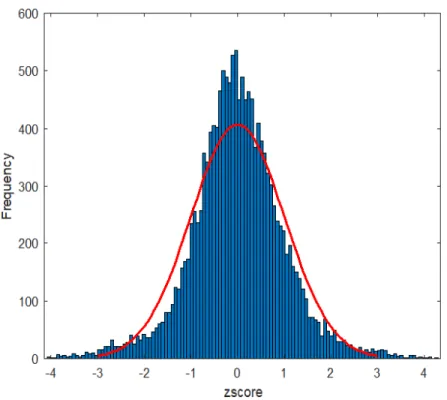
Figure 1: Histogram of z-scores of the weight vector.

integrated impact of each gene in the data over the depth of the SSCAE can be formulated as follows: DM=IW> L Y i=1 LW>_i . (5)

which results in a d×1 weight vector called DM, where d corresponds to the number of features in the original datasets so that each feature has a weight score that reflects its contribution. The weight vector DMresembles a normal distribution as shown in Figure 1 of ovarian cancer dataset at fold 1 of the cross validation procedure. A small percentage of features in theDM

exhibit High Positive (HP) or High Negative (HN) weight as shown in Figure 1. Two lists of features with a length of the bottleneck code (i.e. 50): 1) with HP weight and 2) with HN weight are detected from DM. To examine the consistency of feature selection of the proposed SSCAE over variant training

datasets,kweight vectorsDMsare obtained over cross validation iterations, thus k lists of genes with HP weights and k lists of genes with HN weights are generated. The positive lists are compared to find the most frequently selected predictors with HP weight and the negative lists are examined to identify the most consistently detected predictors with HN weight.

5. Experimental Methodology

This section focuses on the datasets and the experimental methodolo-gies used for model fitting and selection and therefore to validate the out-comes of the proposed SSCAE together with the deep mining model. The datasets used for the evaluation are initially described followed by experimen-tal methodologies adopted, including the applied validation and evaluation metrics.

5.1. Dataset

The development of the breakthroughs for extracting useful knowledge from high-throughput omics data is at the core of personalised and precision medicine. However, we are able to benefit from these biological data only if they are publicly available. Recently, there is increasing pressure from funding providers and the patient community to gain the maximum benefit from produced data by sharing it with the research community regardless whether biomedical studies are funded publicly or privately [48]. Analysing omics data over several research studies can help to control the risk of false positives, offer possibilities to innovative discoveries, and to report signif-icant and reliable findings [49]. Therefore, two publicly available HDSSS Mass Spectrometry and Microarray datasets are used for the experimental evaluation. They are:

• Ovarian Cancer. This dataset is publicly available on the FDA-NCI Clinical Proteomics Program Databank website1. The high-resolution ovarian cancer dataset was generated using the WCX2 protein array to identify serum (blood-derived) proteomic patterns that differentiate the serum of patients with ovarian cancer from that of women without ovar-ian cancer. It contains 216 samples and 15000 features. Each patient sample has one of the response groups: Normal or Cancer, 121(56%)

observations are derived from cancer patients, where 95(44%) obser-vations are from the normal group. The features of Mass Spectrome-try data represent the ion-intensity levels of the patients at particular mass-charge value.

• METABRIC Breast Cancer. This dataset [50] was generated from METABRIC [51, 52] and downloaded from cBioPortal [53]. The cancer study identifier is (brca metabric), and the name is (METABRIC, Na-ture 2012 & Nat Commun2016). Two response groups that are iden-tified in this research are the status of Estrogen Receptor (ER) and Progesterone Receptor (PR). If breast cancer cells have high ER, the cancer is described as ER-positive (ER+), and if breast cancer cells have high PR, the disease is specified as PR-positive (PR+) cancer. ER and PR expressions have been utilised as robust indicators for the evaluation of breast cancer. All newly diagnosed invasive breast cancer patients and breast cancer recurrences should be examined for both ER and PR according to the recommendations of the American Society of Clinical Oncology and the College of American Pathologists [54]. How-ever, it has been shown that the expression of ER and PR receptors changes during the development of breast cancer and in response to systemic therapies [55]. Several expression profiling studies have illus-trated that the expression of hormone receptors is linked with diverse genetic variations [56, 57, 58]. That means several mutated genes can affect the development and progression of breast cancer and contribute to its heterogeneity [59]. As a result, investigating molecular charac-teristics of the tumours that could act as risk factors of breast cancer is considered a serious aetiologic question [60]. This research project aims to identify key genes that underlie the biological processes of ER and PR receptors.

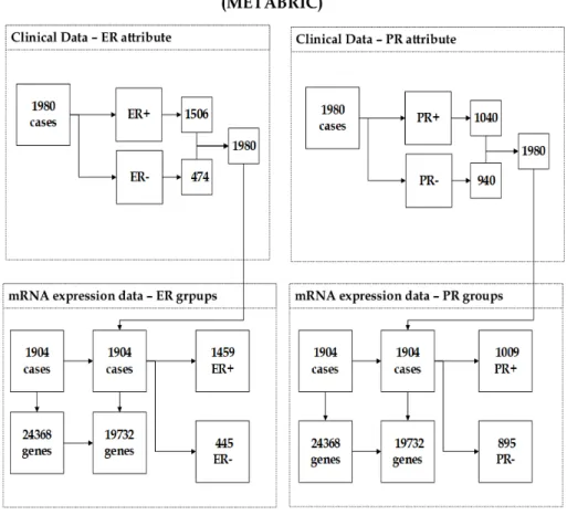
METABRIC dataset contains diverse biomedical modalities including clinical data and two genomic datasets: gene expression, and copy number alterations. The focus of this research is on mRNA expression dataset that was carried out using Illumina Human v3 microarray and contains 24368 genes and 1904 samples as shown in Figure 2. The in-tegration between mRNA expression dataset and ER clinical attribute, which has 1980 cases generated a dataset of 1904, 1459(76.63%) tu-mours were derived from patients with ER+, and 445(23.37%) tumours were derived from ER- samples. Where the unification between mRNA

Figure 2: The description of (METABRIC) dataset showing the unification between clin-ical data and mRNA expression data.

expression dataset and PR clinical data that contains 1980 observations resulted in a dataset of 1904 cases. The number of observations with PR- is 895, so the percentage of PR-negatives is 47.01%, comparing to 1009(52.99%) observations came from patients with PR+ tumours. Gene expression datasets typically contain thousands of genes, not all of these information are relevant. In the microarray literature, several studies have revealed the potential of filtering out genomic datasets from genes with unreliable measurements to enhance the detection of differentially expressed genes [61, 62, 63, 64]. Genes that seem to gen-erate uninformative signals can be considered as noise. A gene with

small profile variance across the samples would not differ significantly among response groups, thus genes with a variance less than the 10th percentile were removed from the analysis in this research. Further-more, gene expression datasets could have genes whose range of values may not well distributed. Therefore, genes with low entropy expres-sion values (i.e less than the 10th percentile) were removed from the analysis in this research. A more detailed discussion of these rudimen-tary filtering methods can be found in [65]. After eliminating the least promising genes from the analysis, the number of remaining features of both response groups ER and PR is 19732 gene profiles as illustrated in Figure 2. This figure provides a summary of the number of samples and genes of mRNA expression dataset before and after the pre-processing step.

5.2. Experimental Methodology

The aim of proposing the SSCAE together with the weight interpretation method is to derive cancer markers whose behaviour differs across conditions, thus they can be used to model reliable prediction systems. Consequently, the generalisability of a machine learning model built on a dataset contain-ing only the informative genes is employed. For small cancer datasets, two powerful but not so adaptable classification models are utilised, which are Support Vector Machine (SVM) [66], and Bagging Decision Tree (BDT) [67] to evaluate the quality of the discovered biomarkers. These learning tech-niques are selected due to their empirical power and success in the same or similar domains. Generalisability of classification models can be defined as its ability to correctly estimate the response groups of unobserved sample cases – (that were not included in the training data). The Area Under the Curve (AUC) of the Receiver Operating Characteristics (ROC) is utilised for estimating the predictive performance of the learning methods. AUC is more reliable than accuracy and more discriminative than other estimation measures and can be measured over the range of TPR and FPR [68, 69]. AUC resides in the range of [0, 1] if the AUC value is equal to 1, it means the predictive performance is perfect (i.e. the classification model correctly assigned all the unseen new cases). If AUC = 0.5 refers to classification by chance (random guessing), and AUC = 0 refers to an inverted perfect clas-sification. In this work, the AUC metric measures the overall quality of the prediction systems with 0.99 confidence level.

Estimation of the predictive performance of learning models is an essen-tial step, since it guides the process of model selection, and evaluates the goodness of the chosen model. For model selection and evaluation, a re-peated 5-fold cross validation procedure is utilised. The 5−fold CV method is empirically established due to achieving a good compromise when at-tempting to address the Bias-Variance trade-off for small cancer datasets. Each dataset is partitioned into 5 non-overlapping subsets of equal size

P ={p1, p2, , p3, p4, p5}. The data subsets are stratified so that each fold

con-tains approximately the same proportions of response groups as in the origi-nal data, and there is evidence that this can enhance the estimation process [70]. The SSCAE is repeated 5 iterations, at each iteration i∈ {1,2,3,4,5}, the SSCAE is applied on P \pi. Over iterations, a set of subsets of

fea-tures F S ={f s1, f s2, f s3, f s4, f s5} is produced. When F S is obtained, the

consistency of feature preferences of the proposed SSCAE is examined by comparing the subsets of features in F S to define the most frequently se-lected features. The consistency of selection is more likely correlated with the predictive power of features so that the most consistency selected fea-tures should be most relevant, whereas the least consistency selected feafea-tures should be less relevant.

6. Results and Discussion

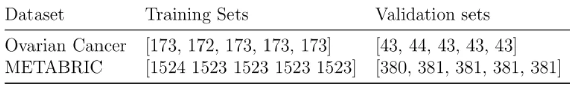
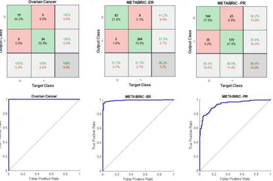
This section evaluates the performance of the proposed SSCAE and deep mining model applied to ovarian and METABRIC breast cancer datasets. Initially, the stratified 5−fold cross validation procedure was utilised to divide each dataset randomly into training sets and validation sets as shown in Table 1. At each iteration, the SSCAE model was trained using the training set and validated using the corresponding validation set as shown in Figure 3 -represented by the confusion matrices and the ROC curve plots for the final iteration. The average predictive performance of that deep feature learning model quantified by AUC is shown in Table 2.

Table 1: The sizes of the training-validation sets of ovarian and METABRIC datasets

Dataset Training Sets Validation sets

Ovarian Cancer [173, 172, 173, 173, 173] [43, 44, 43, 43, 43] METABRIC [1524 1523 1523 1523 1523] [380, 381, 381, 381, 381]

Figure 3: The validation performance of the SSCAE at the final iteration for ovarian cancer, METABRIC with ER groups, and METABRIC with PR groups.

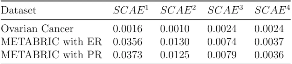
The outcomes of our experiments reveal that the SSCAE was able to learn highly abstract and invariant features from cancer datasets, and thus highly accurate and reliable prediction models were formed. Furthermore, the performance of each trained SCAE module was examined at each cross validation iteration using the MSE between the validation set and its re-construction, which was predicted by the SCAE that was trained on the corresponding training set. Over iterations, the average performance of each SCAE quantified by the MSE is shown in Table 3.

Table 2: The average performance of the SSCAE of ovarian and METABRIC datasets.

Dataset AUC

Ovarian Cancer 0.9843

METABRIC with ER 0.9884 METABRIC with PR 0.9380

Table 3: The average MSE of each SCAE of ovarian cancer and METABRIC datasets.

Dataset SCAE1 SCAE2 SCAE3 SCAE4

Ovarian Cancer 0.0016 0.0010 0.0024 0.0024

METABRIC with ER 0.0356 0.0130 0.0074 0.0037

METABRIC with PR 0.0373 0.0125 0.0079 0.0036

Simultaneously, the proposed deep mining model was applied at each iteration to define two lists of features with HP and HN weight. Over the cross validation iterations, the five identified groups of features with HP weight were compared to provide a subset of stable predictors and by the same way, a subset of stable predictors with HN weight was produced. The experimental results of applying the ensemble deep mining model to ovarian cancer dataset will be discussed first in the following section followed by the outcomes of METABRIC breast cancer dataset with ER and PR groups.

6.1. Results of Ovarian Cancer Dataset

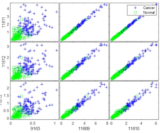
The examination of the ten obtained lists of candidate features of ovarian cancer dataset resulted in finding 6 robust biomarkers with HP weight as shown in the matrix of scatter plots of these biomarkers in Figure 4. The biomarkers were plotted in X-axis and Y-axis ascendingly using their index as illustrated in Figure 4. It can be observed from this figure that the in-tensity distributions of the proteins with HP weight differ significantly for the cancer patients from those from the normal group. Moreover, 13 robust biomarkers were detected from comparing the identified groups of candidate proteins with HN weight as shown in Figure 5. As mentioned previously, the biomarkers were plotted in X-axis and Y-axis ascendingly using their index. It can also be observed from this figure that the intensity distributions of the proteins with HN weight for the observations in the cancer group differ significantly from those in the normal group. Typical biomarkers identifi-cation models adopt the principle that the expression levels of genes or the intensity values of proteins that exhibit the greatest variations across the differentiated groups can be considered as potential biomarkers for a disease or clinically relevant outcome. Therefore, the detected proteins with HP and HN weight could act as potential biomarkers for ovarian cancer.

The discovered subsets of robust biomarkers with HP and HN weight were utilised individually and collectively to develop prediction models using

Figure 4: Scatter plots matrix of the discovered biomarkers (index) with HP weight of ovarian cancer dataset.

the SVM and BDT classifiers. The average predictive performance of both classification models is presented in Table 4. The outcomes of our experiment show that the ensemble subset of HP and HN weighted proteins (i.e. All) contributed to constructing highly accurate and reliable prediction systems.

Table 4: The average performance of the SVM and ENS models built on the subsets of biomarkers of ovarian cancer dataset.

The subset of SVM BDT

HP biomarkers 0.8886 0.8726 HN biomarkers 0.8975 0.8828 All biomarkers 0.9227 0.8964

Figure 5: Scatter plots matrix of the discovered biomarkers (index) with HN weight of ovarian cancer dataset.

Our findings demonstrate first the efficiency of the proposed SSCAE to capture intrinsic structure in serum (blood)-derived proteomic data. Sec-ondly, it is a strong indicator that the proposed deep mining model was able to deconstruct the SSCAE and interpret its weight matrices effectively so that the proteomic patterns that can differentiate the patients with ovarian cancer from the women without ovarian cancer were detected in two forms.

6.2. Results of METABRIC Breast Cancer Dataset

This section evaluates the performance of the proposed deep mining model applied to analyse the weight matrices of the SSCAE built on METABRIC dataset with ER and PR groups for the goal of discovering robust biomarkers that are positively and negatively associated with the hormone receptors.

Figure 6: Scatter plots matrix of the discovered biomarkers with HN weight of METABRIC dataset with ER groups.

6.2.1. Results of ER Groups

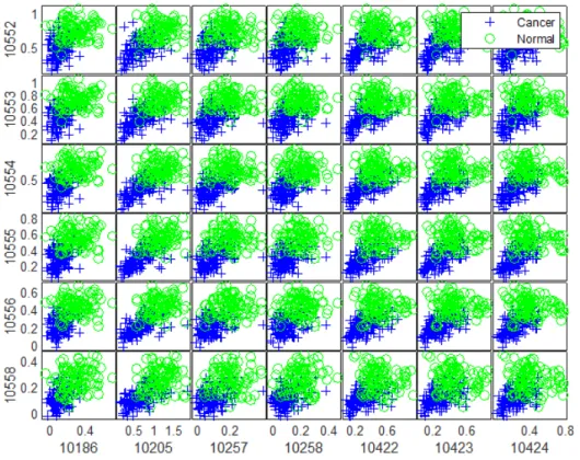
The application of the ensemble deep mining model to METABRIC dataset with ER groups resulted in defining 25 robust biomarkers with HP weight as shown in Figure 7. Furthermore, 7 robust biomarkers were detected from the identified subsets of candidate genes with HN weight as shown in Figure 6. The mRNA markers were plotted in X-axis and Y-axis alphabetically using their names as shown in Figures 6 and 7. It can be observed in both figures that the expression levels of the recognised genes for the patient with ER+ tumours differ significantly from the samples with ER- tumours. Therefore,

the detected mRNA markers with HP and HN weight could act as potential biomarkers for breast cancer and ER positivity.

Figure 7: Scatter plots matrix of the disco v ered biomark ers with HP w eigh t of MET ABRIC dataset with ER groups.

Figure 8: Scatter plots matrix of the discovered biomarkers with HP weight of METABRIC dataset with PR groups.

6.2.2. Results of PR Group

The application of the ensemble deep mining model to METABRIC data with PR groups led to identifying 6 robust biomarkers with HP weight as shown in Figure 8. Furthermore, 5 mRNA markers were found to be neg-atively associated with PR positivity as shown in Figure 9. The discov-ered mRNAs were plotted in X-axis and Y-axis alphabetically using their names as illustrated in Figures 8 and 9. As shown clearly in these figures, the mRNA markers exhibit distinct expression levels for the patient with PR+ tumours from the samples with PR-negative tumours. Therefore, the discovered mRNA markers with HP and HN weight could act as potential biomarkers for breast cancer and high PR level.

Figure 9: Scatter plots matrix of the discovered biomarkers with HN weight of METABRIC dataset with PR groups.

models individually and as an ensemble using the SVM and BDT methods. The average predictive performance of both classifiers is presented in Table 5. For ER groups, the outcomes of our experiment reveal that the HP weighted biomarkers of METABRIC dataset built highly accurate and robust classi-fication models than HN weighted genes. Furthermore, the integration of the subsets of mRNA markers has improved the predictive performance of the SVM model only and very slightly. Similar findings were also obtained from the METABRIC dataset with PR groups where the predictive perfor-mance of the classification models built on the HP weighted biomarkers is significantly higher than its performance when trained using mRNAs with HN weight. Moreover, the ensemble subset of the discovered biomarkers has improved the performance of the BDT model only and very slightly.

Table 5: The average performance of the SVM and ENS models built on the subsets of biomarkers of METABRIC datasets.

The subset of SVM BDT

HP biomarkers with ER 0.9820 0.9853 HN biomarkers with ER 0.9023 0.8838 All biomarkers with ER 0.9855 0.9850 HP biomarkers with PR 0.9825 0.9815 HN biomarkers with PR 0.7290 0.7143 All biomarkers with PR 0.9815 0.9824

6.3. Discussion

The outcomes of our experiments for ovarian cancer dataset have shown how the intensity values of the detected proteins with HP weight differ signif-icantly from the intensity values of the discovered proteins with HN weight for the cancer and normal samples. More specifically, the intensity values of the selected proteins with HP weight for the patients who suffer from cancer are more likely to be higher than most of the normal samples as shown in Figure 4. Contrary to the intensity distributions of the discovered proteins with HN weight, where their intensity values for the normal observations are more likely to be higher than most of the cancer samples as illustrated in Figure 5. Firstly, this is strong evidence that validates the effectiveness of the SSCAE to capture the interesting complexity in serum (blood)-derived proteomic data. Secondly, it is a strong indicator that demonstrates the ca-pability of the proposed deep mining model to deconstruct the internal state of the SSCAE effectively so that the salient and robust proteomic signals that are positively and negatively associated with ovarian cancer were discovered robustly.

The experimental results of METABRIC dataset with ER groups have shown how the expression levels of the discovered genes with HP weight differ significantly from the expression levels of the HN weighted mRNA markers for ER+ and ER- samples. More specifically, our findings reveal that the expression levels of HP weighted mRNA markers are more likely to be higher for the patients with ER+ tumours compared to most of the ER-negatives as shown in Figure 7. In contrast, the identified mRNAs with HN weight exhibit higher expression levels for the observations from the ER- group in comparison to the ER-positive patients as shown in Figure 6. This provides

another great evidence that verifies the efficacy of the proposed SSCAE to discover useful knowledge from this HDSSS genomic data as well as the potential of the deep mining model to interpret the weight matrices of the SSCAE and recognise robust biomarkers that are positively and negatively associated with breast cancer and ER positivity.

The experimental outcomes of METABRIC dataset with PR groups have explained the significant differences in the expression levels of the discovered biomarkers with HP weight from the HN weighted mRNAs for PR+ and PR- samples. It has been shown in this research that the patients with PR+ tumours are more likely characterised with high expression levels of the selected mRNAs with HP weight compared to the samples from the PR-group as presented in Figure 8. In contrast, mRNA markers with HN weight exhibit low expression levels for patients with PR+ tumours in comparison to most of the PR- samples as explained in Figure 9. This is a strong indicator that verifies the capability of the SSCAE to learn high-level abstract features from this HDSSS genomic dataset. Moreover, this is significant evidence that supports the validity of the presented deep mining model to open the black box of that deep feature learning model and discover interesting patterns that are associated with breast cancer and high PR levels positively and negatively.

Our findings reveal conclusive evidence of a positive or a negative asso-ciation between each single biomarker and its response group. The positive association was observed between the discovered genes or proteins with HP weight and the positive response group (i.e. Cancer, ER+, PR+) as shown in Figures 4, 7, 8. The positive correlation corresponds to the gains in the expression/intensity levels of these biomarkers and its contribution to cancer-ous of ovarian or ER/PR positivity. The inverse correlation was recognised between the identified genes or proteins with HN weight and the positive response group (i.e. Cancer, ER+, PR+) as shown in Figures 5, 6, 9. The negative correlation refers to the declines in the expression/intensity levels of these biomarkers and its contribution to ovarian cancer and ER/PR posi-tivity. This provides very strong evidence that validates the potential of our deep mining model to interpret the weight matrices of the SSCAE by finding generic features that exhibit HP and HN weight scores. In addition, this also reflects the capability of the SSCAE in assigning correctly HP weight to the biomarkers that are highly expressed for the positive patients compared to the negative samples, and HN weight to the biomarkers that are lowly expressed for the positive patients in comparison to the negatives.

Our computational study that aims for knowledge discovery from omics data focuses mainly on data modelling, analysis, and validation that allow new sets of biomarkers for ovarian and breast cancers to be discovered effi-ciently and validated reliably. The discovered molecular markers could an-swer different biological questions of interest and contribute to developing more personalised treatment or monitoring planning by investigating further the mechanism underlying the association of expression patterns of these biomarkers and the cancers of interest. Our novel deep mining model pro-vides yet another arrow within the quiver of bioinformaticians for discovering and evaluating new biomarkers that may help further the endeavor of pro-ducing more effective and personalised medicine.

7. Conclusions

The process of inferring useful knowledge from HDSSS omics data poses several critical issues that arise due to experimental, statistical and compu-tational challenges. The limitations of existing approaches established by the literature review drive us to critically assess the usefulness of deep neural network methods for the problem of knowledge discovery from high through-put omics data. The critical evaluation has resulted in defining the key requirements for a deep feature learning model to be able to capture enough of the important variations underlying the representative biological samples. Consequently, we introduce the proposal of the SSCAE for the extraction and analysis of reliable knowledge from human molecular data for modelling robust prediction systems.

The deep mining model is proposed to open the black-box of the SSCAE and find robustly which genes were dominant within its internal represen-tations. The detailed evaluation of the deep mining model demonstrates its capacity to recognise the biomarkers that exhibit HP or HN weight scores over the depth of the network. HP weighted biomarkers are the molecules that have a strong positive correlation with the positive group, where HN weighted biomarkers are the molecules that have an inverse association with the positive group. This explains the internal mechanism of the SSCAE in assigning HP weight to the features that are highly expressed for the posi-tives in comparison to most of the negaposi-tives. In contrast, HN weights were allocated by the SSCAE to the features that are lowly expressed for most of the positives in comparison to the negatives. The validation process reveal that the discovered biomarkers demonstrate computational and biological

relevance as well as the capability to construct highly accurate and reliable prediction models. This provides significant evidence that the deep mining model was very effective in offering explainability to the deep learning model and detecting key determinants underlying its latent representations.

In the next publication, the capacity of the proposed deep feature min-ing model to detect generic biomarkers for breast cancer from a wide range of independently generated cancer genomic samples that are collected from completely different studies is investigated so that the highest evidence that a tool validates can be provided. As mentioned previously, our deep min-ing model is problem-independent and data-driven, thus, it provides further potential for this research to extend beyond its cognate disciplines.

Conflict of interest statement

There is no conflict of interest.

References

[1] B. D. W. Group, A. J. Atkinson Jr, W. A. Colburn, V. G. DeGruttola, D. L. DeMets, G. J. Downing, D. F. Hoth, J. A. Oates, C. C. Peck, R. T. Schooley, et al., Biomarkers and surrogate endpoints: preferred defini-tions and conceptual framework, Clinical Pharmacology & Therapeutics 69 (3) (2001) 89–95.

[2] D. C. Collins, R. Sundar, J. S. Lim, T. A. Yap, Towards precision medicine in the clinic: from biomarker discovery to novel therapeutics, Trends in pharmacological sciences 38 (1) (2017) 25–40.

[3] F. Vafaee, C. Diakos, M. B. Kirschner, G. Reid, M. Z. Michael, L. G. Horvath, H. Alinejad-Rokny, Z. J. Cheng, Z. Kuncic, S. Clarke, A data-driven, knowledge-based approach to biomarker discovery: application to circulating microrna markers of colorectal cancer prognosis, NPJ sys-tems biology and applications 4 (1) (2018) 20.

[4] Y. Bengio, Deep learning of representations for unsupervised and trans-fer learning, in: Proceedings of ICML Workshop on Unsupervised and Transfer Learning, 2012, pp. 17–36.

[5] H. Larochelle, D. Erhan, A. Courville, J. Bergstra, Y. Bengio, An em-pirical evaluation of deep architectures on problems with many factors of variation, in: Proceedings of the 24th international conference on Machine learning, ACM, 2007, pp. 473–480.

[6] Y. Bengio, et al., Learning deep architectures for ai, Foundations and trendsR in Machine Learning 2 (1) (2009) 1–127.

[7] D. Erhan, Y. Bengio, A. Courville, P.-A. Manzagol, P. Vincent, S. Ben-gio, Why does unsupervised pre-training help deep learning?, Journal of Machine Learning Research 11 (Feb) (2010) 625–660.

[8] V. E. Bichsel, L. A. Liotta, et al., Cancer proteomics: from biomarker discovery to signal pathway profiling., Cancer journal (Sudbury, Mass.) 7 (1) (2001) 69–78.

[9] G. E. Hinton, Connectionist learning procedures, in: Machine Learning, Volume III, Elsevier, 1990, pp. 555–610.

[10] D. E. Rumelhart, J. L. McClelland, Parallel distributed processing: ex-plorations in the microstructure of cognition. volume 1. foundations. [11] Y. LeCun, Y. Bengio, G. Hinton, Deep learning, nature 521 (7553)

(2015) 436.

[12] J. Zhou, O. G. Troyanskaya, Predicting effects of noncoding variants with deep learning–based sequence model, Nature methods 12 (10) (2015) 931.

[13] D. R. Kelley, J. Snoek, J. L. Rinn, Basset: learning the regulatory code of the accessible genome with deep convolutional neural networks, Genome research.

[14] C. Angermueller, H. Lee, W. Reik, O. Stegle, Accurate prediction of single-cell dna methylation states using deep learning, BioRxiv (2017) 055715.

[15] P. W. Koh, E. Pierson, A. Kundaje, Denoising genome-wide histone chip-seq with convolutional neural networks, Bioinformatics 33 (14) (2017) i225–i233.

[16] B. Alipanahi, A. Delong, M. T. Weirauch, B. J. Frey, Predicting the sequence specificities of dna-and rna-binding proteins by deep learning, Nature biotechnology 33 (8) (2015) 831.

[17] T. Brosch, R. Tam, A. D. N. Initiative, et al., Manifold learning of brain mris by deep learning, in: International Conference on Medical Image Computing and Computer-Assisted Intervention, Springer, 2013, pp. 633–640.

[18] S. Liu, S. Liu, W. Cai, S. Pujol, R. Kikinis, D. Feng, Early diagnosis of alzheimer’s disease with deep learning, in: Biomedical Imaging (ISBI), 2014 IEEE 11th International Symposium on, IEEE, 2014, pp. 1015– 1018.

[19] Y. Yoo, T. Brosch, A. Traboulsee, D. K. Li, R. Tam, Deep learning of image features from unlabeled data for multiple sclerosis lesion seg-mentation, in: International Workshop on Machine Learning in Medical Imaging, Springer, 2014, pp. 117–124.

[20] J.-Z. Cheng, D. Ni, Y.-H. Chou, J. Qin, M. Tiu, Y.-C. Chang, C.-S. Huang, D. Shen, C.-M. Chen, Computer-aided diagnosis with deep learning architecture: applications to breast lesions in us images and pulmonary nodules in ct scans, Scientific reports 6 (2016) 24454. [21] R. Miotto, L. Li, B. A. Kidd, J. T. Dudley, Deep patient: an

unsuper-vised representation to predict the future of patients from the electronic health records, Scientific reports 6 (2016) 26094.

[22] T. Tran, T. D. Nguyen, D. Phung, S. Venkatesh, Learning vector repre-sentation of medical objects via emr-driven nonnegative restricted boltz-mann machines (enrbm), Journal of biomedical informatics 54 (2015) 96–105.

[23] T. Pham, T. Tran, D. Phung, S. Venkatesh, Deepcare: A deep dynamic memory model for predictive medicine, in: Pacific-Asia Conference on Knowledge Discovery and Data Mining, Springer, 2016, pp. 30–41. [24] N. Y. Hammerla, S. Halloran, T. Ploetz, Deep, convolutional, and

re-current models for human activity recognition using wearables, arXiv preprint arXiv:1604.08880.

[25] J. Zhu, A. Pande, P. Mohapatra, J. J. Han, Using deep learning for energy expenditure estimation with wearable sensors, in: E-health Net-working, Application & Services (HealthCom), 2015 17th International Conference on, IEEE, 2015, pp. 501–506.

[26] A. Sathyanarayana, S. Joty, L. Fernandez-Luque, F. Ofli, J. Srivastava, A. Elmagarmid, T. Arora, S. Taheri, Correction of: sleep quality pre-diction from wearable data using deep learning, JMIR mHealth and uHealth 4 (4).

[27] A. Krizhevsky, I. Sutskever, G. E. Hinton, Imagenet classification with deep convolutional neural networks, in: Advances in neural information processing systems, 2012, pp. 1097–1105.

[28] C. Szegedy, W. Liu, Y. Jia, P. Sermanet, S. Reed, D. Anguelov, D. Er-han, V. Vanhoucke, A. Rabinovich, Going deeper with convolutions, in: Proceedings of the IEEE conference on computer vision and pattern recognition, 2015, pp. 1–9.

[29] R. Collobert, J. Weston, L. Bottou, M. Karlen, K. Kavukcuoglu, P. Kuksa, Natural language processing (almost) from scratch, Journal of Machine Learning Research 12 (Aug) (2011) 2493–2537.

[30] I. Sutskever, O. Vinyals, Q. V. Le, Sequence to sequence learning with neural networks, in: Advances in neural information processing systems, 2014, pp. 3104–3112.

[31] G. Hinton, L. Deng, D. Yu, G. E. Dahl, A.-r. Mohamed, N. Jaitly, A. Senior, V. Vanhoucke, P. Nguyen, T. N. Sainath, et al., Deep neural networks for acoustic modeling in speech recognition: The shared views of four research groups, IEEE Signal processing magazine 29 (6) (2012) 82–97.

[32] O. Abdel-Hamid, A.-r. Mohamed, H. Jiang, L. Deng, G. Penn, D. Yu, Convolutional neural networks for speech recognition, IEEE/ACM Transactions on audio, speech, and language processing 22 (10) (2014) 1533–1545.

[33] L. Deng, X. Li, Machine learning paradigms for speech recognition: An overview, IEEE Transactions on Audio, Speech, and Language Process-ing 21 (5) (2013) 1060–1089.

[34] S. Wang, D. Quan, X. Liang, M. Ning, Y. Guo, L. Jiao, A deep learn-ing framework for remote senslearn-ing image registration, ISPRS Journal of Photogrammetry and Remote Sensing.

[35] Q. Zou, L. Ni, T. Zhang, Q. Wang, Deep learning based feature selection for remote sensing scene classification., IEEE Geosci. Remote Sensing Lett. 12 (11) (2015) 2321–2325.

[36] P. Vincent, H. Larochelle, I. Lajoie, Y. Bengio, P.-A. Manzagol, Stacked denoising autoencoders: Learning useful representations in a deep net-work with a local denoising criterion, Journal of machine learning re-search 11 (Dec) (2010) 3371–3408.

[37] G. E. Hinton, S. Osindero, Y.-W. Teh, A fast learning algorithm for deep belief nets, Neural computation 18 (7) (2006) 1527–1554.

[38] Y. Bengio, P. Lamblin, D. Popovici, H. Larochelle, Greedy layer-wise training of deep networks, in: B. Sch¨olkopf, J. C. Platt, T. Hoffman (Eds.), Advances in Neural Information Processing Systems 19, MIT Press, 2007, pp. 153–160.

[39] C. Poultney, S. Chopra, Y. L. Cun, et al., Efficient learning of sparse representations with an energy-based model, in: Advances in neural information processing systems, 2007, pp. 1137–1144.

[40] J. Tan, M. Ung, C. Cheng, C. S. Greene, Unsupervised feature construc-tion and knowledge extracconstruc-tion from genome-wide assays of breast cancer with denoising autoencoders, in: Pacific Symposium on Biocomputing Co-Chairs, World Scientific, 2014, pp. 132–143.

[41] J. Tan, J. H. Hammond, D. A. Hogan, C. S. Greene, Adage-based in-tegration of publicly available pseudomonas aeruginosa gene expression data with denoising autoencoders illuminates microbe-host interactions, MSystems 1 (1) (2016) e00025–15.

[42] P. Danaee, R. Ghaeini, D. A. Hendrix, A deep learning approach for cancer detection and relevant gene identification, in: PACIFIC SYM-POSIUM ON BIOCOMPUTING 2017, World Scientific, 2017, pp. 219– 229.

[43] R. Fletcher, Practical methods of optimization, John Wiley & Sons, 2013.

[44] M. R. Hestenes, Conjugate direction methods in optimization, Vol. 12, Springer Science & Business Media, 2012.

[45] M. J. D. Powell, Restart procedures for the conjugate gradient method, Mathematical programming 12 (1) (1977) 241–254.

[46] P. E. Gill, W. Murray, Safeguarded steplength algorithms for optimiza-tion using descent methods, Naoptimiza-tional Physical Laboratory, Division of Numerical Analysis and Computing, 1974.

[47] M. F. Møller, A scaled conjugate gradient algorithm for fast supervised learning, Neural networks 6 (4) (1993) 525–533.

[48] N. V. Kovalevskaya, C. Whicher, T. D. Richardson, C. Smith, J. Grajcia-rova, X. Cardama, J. Moreira, A. Alexa, A. A. McMurray, F. G. Nielsen, Dnadigest and repositive: connecting the world of genomic data, PLoS biology 14 (3) (2016) e1002418.

[49] F. S. Collins, L. A. Tabak, Nih plans to enhance reproducibility, Nature 505 (7485) (2014) 612–613.

[50] B. Pereira, S.-F. Chin, O. M. Rueda, H.-K. M. Vollan, E. Provenzano, H. A. Bardwell, M. Pugh, L. Jones, R. Russell, S.-J. Sammut, et al., The somatic mutation profiles of 2,433 breast cancers refine their genomic and transcriptomic landscapes, Nature communications 7 (2016) 11479. [51] C. Curtis, S. P. Shah, S.-F. Chin, G. Turashvili, O. M. Rueda, M. J. Dunning, D. Speed, A. G. Lynch, S. Samarajiwa, Y. Yuan, et al., The genomic and transcriptomic architecture of 2,000 breast tumours reveals novel subgroups, Nature 486 (7403) (2012) 346.

[52] S.-J. Dawson, O. M. Rueda, S. Aparicio, C. Caldas, A new genome-driven integrated classification of breast cancer and its implications, The EMBO journal 32 (5) (2013) 617–628.

[53] J. Gao, B. A. Aksoy, U. Dogrusoz, G. Dresdner, B. Gross, S. O. Sumer, Y. Sun, A. Jacobsen, R. Sinha, E. Larsson, et al., Integrative analysis of complex cancer genomics and clinical profiles using the cbioportal, Sci. Signal. 6 (269) (2013) pl1–pl1.

[54] M. E. H. Hammond, D. F. Hayes, M. Dowsett, D. C. Allred, K. L. Hagerty, S. Badve, P. L. Fitzgibbons, G. Francis, N. S. Goldstein, M. Hayes, et al., American society of clinical oncology/college of amer-ican pathologists guideline recommendations for immunohistochemi-cal testing of estrogen and progesterone receptors in breast cancer (unabridged version), Archives of pathology & laboratory medicine 134 (7) (2010) e48–e72.

[55] A. J. Lowery, N. Miller, A. Devaney, R. E. McNeill, P. A. Davoren, C. Lemetre, V. Benes, S. Schmidt, J. Blake, G. Ball, et al., Microrna sig-natures predict oestrogen receptor, progesterone receptor and her2/neu receptor status in breast cancer, Breast cancer research 11 (3) (2009) R27.

[56] C. M. Perou, T. Sørlie, M. B. Eisen, M. Van De Rijn, S. S. Jeffrey, C. A. Rees, J. R. Pollack, D. T. Ross, H. Johnsen, L. A. Akslen, et al., Molecular portraits of human breast tumours, nature 406 (6797) (2000) 747.

[57] T. Sørlie, C. M. Perou, R. Tibshirani, T. Aas, S. Geisler, H. Johnsen, T. Hastie, M. B. Eisen, M. Van De Rijn, S. S. Jeffrey, et al., Gene ex-pression patterns of breast carcinomas distinguish tumor subclasses with clinical implications, Proceedings of the National Academy of Sciences 98 (19) (2001) 10869–10874.

[58] T. Sørlie, R. Tibshirani, J. Parker, T. Hastie, J. S. Marron, A. Nobel, S. Deng, H. Johnsen, R. Pesich, S. Geisler, et al., Repeated observation of breast tumor subtypes in independent gene expression data sets, Pro-ceedings of the national academy of sciences 100 (14) (2003) 8418–8423. [59] S. M. Bernhardt, P. Dasari, D. Walsh, A. R. Townsend, T. J. Price, W. V. Ingman, Hormonal modulation of breast cancer gene expression: implications for intrinsic subtyping in premenopausal women, Frontiers in oncology 6 (2016) 241.

[60] M. Garcia-Closas, S. Chanock, Genetic susceptibility loci for breast can-cer by estrogen receptor status, Clinical Cancan-cer Research 14 (24) (2008) 8000–8009.

[61] R. Gentleman, V. Carey, W. Huber, R. Irizarry, S. Dudoit, Bioinfor-matics and computational biology solutions using R and Bioconductor, Springer Science & Business Media, 2006.

[62] J. N. McClintick, H. J. Edenberg, Effects of filtering by present call on analysis of microarray experiments, BMC bioinformatics 7 (1) (2006) 49.

[63] W. Talloen, D.-A. Clevert, S. Hochreiter, D. Amaratunga, L. Bijnens, S. Kass, H. W. G¨ohlmann, I/ni-calls for the exclusion of non-informative genes: a highly effective filtering tool for microarray data, Bioinformatics 23 (21) (2007) 2897–2902.

[64] D. Tritchler, E. Parkhomenko, J. Beyene, Filtering genes for cluster and network analysis, BMC bioinformatics 10 (1) (2009) 193.

[65] I. S. Kohane, A. J. Butte, A. Kho, Microarrays for an integrative ge-nomics, MIT press, 2002.

[66] B. E. Boser, I. M. Guyon, V. N. Vapnik, A training algorithm for opti-mal margin classifiers, in: Proceedings of the fifth annual workshop on Computational learning theory, ACM, 1992, pp. 144–152.

[67] L. Breiman, Bagging predictors, Machine learning 24 (2) (1996) 123– 140.

[68] C. X. Ling, J. Huang, H. Zhang, Auc: a better measure than accuracy in comparing learning algorithms, in: Conference of the canadian society for computational studies of intelligence, Springer, 2003, pp. 329–341. [69] C. X. Ling, J. Huang, H. Zhang, et al., Auc: a statistically consistent

and more discriminating measure than accuracy, in: IJCAI, Vol. 3, 2003, pp. 519–524.

[70] I. H. Witten, E. Frank, Data mining practical learning tools and tech-niques with java implementations (2000).