JOINT MODELING OF BIVARIATE TIME TO EVENT
DATA WITH SEMI-COMPETING RISK
Ran Liao
Submitted to the faculty of the University Graduate School in partial fulfillment of the requirements
for the degree Doctor of Philosophy
in the Department of Biostatistics, Indiana University
Accepted by the Graduate Faculty, Indiana University, in partial fulfillment of the requirements for the degree of Doctor of Philosophy.
Doctoral Committee
September 8, 2016
Sujuan Gao, Ph.D., Chair
Barry Katz, Ph.D.
Ying Zhang, Ph.D.
Shanshan Li, M.D.
c 2017 Ran Liao
DEDICATION
ACKNOWLEDGMENTS
While a completed dissertation bears the single name of the student, the pro-cess that leads to its completion is always accomplished in combination with the dedicated work of other people. I owe my gratitude to all those people who made this dissertation possible and because of whom my doctoral experience has been one that I will cherish forever.
First and foremost I want to thank my advisor and committee chair, Profes-sor Sujuan Gao, who continually and convincingly conveyed a spirit of adventure in regard to research and scholarship. Without her guidance and persistent help, this dissertation would not have been possible. It has been an honor to be her Ph.D. student. She has taught me, both intentionally and unintentionally, how good a bio-statistician and a researcher could be. I appreciate all her contributions of time, ideas, and funding to make my Ph.D. experience productive and stimulating. The joy and enthusiasm she has for her research and projects was appealing and motivational for me, even during tough times in the Ph.D. pursuit. I am also thankful for the excellent example she has provided as a successful female biostatistician and researcher. Her guidance will accompany me along my life, especially my journey in biostatistics, and I will continue to benefit from it.
I would like to gratefully and sincerely thank my committee members: Dr.Barry Katz, Dr. Ying Zhang, Dr.Shanshan Li and Dr. Jianjun Zhang. First, I would like to give my special thanks to Dr. Barry Katz, Chair of Biostatistics Department and Dr. Ying Zhang, Director of Biostatistics Program, for their constant effort in improving our program and providing so many wonderful opportunities for students
and junior researchers. Additionally, I want to thank Dr. Katz for his instruction and advice during classes and discussion. He showed me the way to make significant contributions to society by conducting biostatistics research that is critical in fighting disease. Thanks to Dr. Ying Zhang for his extensive knowledge in survival analysis and counting process; our discussion regarding likelihood, frailty model, and twostage model gave me a clear picture of methodologies in these areas. Thanks to Dr. Shan-shan Li for her creative and cutting edge knowledge in joint modeling of survival data and longitudinal data analysis, and also in dynamic prediction. It has been great opportunity for me to learn these methodologies when I sit in the LiveAD project meeting. Thanks to Dr. Jianjun Zhang who is also my minor advisor; his instructions and knowledge in cancer epidemiology and nutrition epidemiology inspired me and also provoked my interest in oncology, which led me to my future career direction.
It has been wonderful experience to study and work in the Department of Biostatistics at Indiana University. I would like to express my sincere thanks to all the faculty members, biostatisticians and staff in our department, for their input, expertise, valuable discussions, patience, and accessibility. In particular, I would like to thank our department for offering me the chance to collaborate with the Chinese Center of Disease Control and the Regenstrief Institute, which has been a truly precious opportunity for me, where I developed collaboration skills and learned how to apply my knowledge to real world problems. Also I would like to thank Dr. Zhangsheng Yu and Dr.Wanzhu Tu for their assistance and insightful comments to my research work in frailty model. I learned a lot from their previous work and through our research discussions. I also feel thankful for daily help from all the current
and former students in the biostatistics program as well as the students outside the program.
I would like to extend my thanks to Dr.Tianle Hu at Eli Lilly for his support to my “bivariate time to event data association” research. Dr.Hu offered me his insightful knowledge and expertise in this area. I am so honored to work with Dr.Hu and have him as coauthor for some of my research work. And Dr.Hu also enlightened me with the latest progress and methodologies in pharmaceutical industrial and clinical trials, which has been valuable information to direct me in my career path.
I wish to express my thanks to my family and friends. Thanks to my parents and grandparents who raised me up as a positive and energetic person and gave me enough support to let me explore the world. Thanks to my mom Rong Zhang for her unconditional love and endless support. Thanks to my parents in law and grandpar-ents in law for their understanding and encouragement. Thanks to my friends who can accompany me when I am so frustrated with my life and family.
Last, thanks to my dearest husband: Jie Xue. Jie and I are working on our doctorate degree at same time. We went through this journey together; we made each other much braver and stronger in facing challenges and obstacles in life. In the meantime, we are much humbler and more prepared for the uncertainty of the future. And to my daughter, Qixuan Xue (Emma), and possible future kids, let mom share this statistician’s secrete with you: If you determined to get some significance, but it just doesn’t work out. Don’t give up. Try harder and try again, play smarter and play again, you will be pleased by what the persistence and the possibility bring to you during the procedure, and also in the end.
Ran Liao
JOINT MODELING OF BIVARIATE TIME TO EVENT DATA WITH SEMI-COMPETING RISK
Survival analysis often encounters the situations of correlated multiple events including the same type of event observed from siblings or multiple events experienced by the same individual. In this dissertation, we focus on the joint modeling of bivariate time to event data with the estimation of the association parameters and also in the situation of a semi-competing risk.
This dissertation contains three related topics on bivariate time to event mod-els. The first topic is on estimating the cross ratio which is an association parameter between bivariate survival functions. One advantage of using cross-ratio as a depen-dence measure is that it has an attractive hazard ratio interpretation by comparing two groups of interest. We compare the parametric, a two-stage semiparametric and a nonparametric approaches in simulation studies to evaluate the estimation perfor-mance among the three estimation approaches.
The second part is on semiparametric models of univariate time to event with a semi-competing risk. The third part is on semiparametric models of bivariate time to event with semi-competing risks. A frailty-based model framework was used to accommodate potential correlations among the multiple event times. We propose two estimation approaches. The first approach is a two stage semiparametric method where cumulative baseline hazards were estimated by nonparametric methods first
likelihood approach. Simulation studies were conducted to compare the estimation accuracy between the proposed approaches. Data from an elderly cohort were used to examine factors associated with times to multiple diseases and considering death as a semi-competing risk.
TABLE OF CONTENTS
LIST OF TABLES . . . xiv
LIST OF FIGURES . . . xvi
Chapter 1 Introduction . . . 1
1.1 Overview . . . 1
1.2 Covariate Dependent Cross Ratio of Bivariate Survival Times . . 3
1.3 Frailty based Semiparametric Models for Time to Event Data with a Semi-competing Risk . . . 4
1.4 Frailty-based Multi-event Semiparametric Models for Failure Time Data with Semi-competing Risks . . . 6
1.5 Main Contribution and Structure of Dissertation . . . 7
Chapter 2 Covariate Dependent Cross Ratio of Bivariate Survival Times . 9 2.1 Abstract . . . 9
2.2 Introduction . . . 10
2.3 Notation, Definition and Model Setup . . . 13
2.4 Estimation Approaches . . . 17
2.4.1 Bivariate Clayton Copula Approach . . . 18
2.4.2 Two Stage Semiparametric Estimation Approach . . . 22
2.4.3 Nonparametric Pseudo-Partial Likelihood Estimation Approach 25 2.5 Simulation Study . . . 26
2.5.1 Data Setup . . . 27
2.5.3 Simulation Results when the Model is Misspecified . . . . 31
2.6 Data Application: Estimate Gender Effect in Cross Ratio between Time to CAD and Depression . . . 33
2.6.1 Indianapolis-Ibadan African American Cohort . . . 33
2.6.2 Estimate Gender Effect in Cross Ratio between Time to CAD and Depression . . . 35
2.7 Discussion . . . 38
Chapter 3 Frailty-based Semiparametric Models for Time to Event Data with Semi-competing Risk . . . 42
3.1 Abstract . . . 42
3.2 Introduction . . . 43
3.3 Frailty Model in Competing Risk Data and Semi-competing Risk Data . . . 46
3.4 Model and Likelihood . . . 48
3.4.1 Models for Semi-competing Risks Data . . . 48
3.4.2 Likelihood . . . 51
3.5 Estimation Approaches . . . 55
3.5.1 Two Stage Semiparametric Pseudo Likelihood Approach . 55 3.5.2 Penalized Partial Likelihood Estimation . . . 58
3.6 Simulations . . . 62
3.6.1 Simulation Setup . . . 62
3.6.2 Simulation Results . . . 63
3.7 Data Application Example . . . 70
3.9 Event Specific Hazard and Model Setup . . . 72
3.10 Conclusion . . . 73
Chapter 4 Frailty-based Multi-event Semiparametric Models for Failure Time Data with Semi-competing Risks . . . 75
4.1 Abstract . . . 75
4.2 Introduction . . . 75
4.3 Notation and Setup . . . 78
4.4 Review of Current Multi-event and Multi-state Model . . . 79
4.4.1 Parametric and Semiparametric Frailty Model . . . 79
4.4.2 Multi-state Markov Model . . . 80
4.5 Model and Likelihood . . . 81
4.5.1 Path Specific Hazard with Frailty Setup . . . 81
4.5.2 Likelihood . . . 82
4.6 Estimation . . . 89
4.6.1 Two Stage Pseudo-Likelihood Approach . . . 89
4.6.2 Penalized Partial Likelihood Approach . . . 91
4.7 Simulation Study . . . 95
4.7.1 Data Preparation . . . 95
4.7.2 Simulation Results . . . 100
4.8 Application . . . 104
4.9 Conclusion and Discussion . . . 109
Chapter 5 Conclusion and Discussion . . . 110
6.1 More Simulation Results for Covariate Dependent Cross Ratio of
Bivariate Survival Times . . . 114
BIBLIOGRAPHY . . . 118
LIST OF TABLES
2.1 Simulation Result for Covariate Dependent Cross Ratio Estimation
with Correctly Specified Model Scenario: Marginal Survival of T1 and
T2 are Exponential Distribution, the true β = 0.5 . . . 30
2.2 Simulation Result for Covariate Dependent Cross Ratio Estimation
with Mis-specified Model Scenario: Marginal Survival: Marginal
Sur-vival of T1 andT2 are Weibull Distribution with λ= 2, p= 3, the true
β = 0.5. . . 32
2.3 Demographic Characteristic of IIDP Data with Number of Event and
Incidence Rate by Each Gender Group . . . 34
2.4 Median Age Onset for Each Disease by Gender and the Status of the
Other Disease . . . 35
2.5 Estimates of Covariate Dependent Cross Ratio and Gender Effect in
IIDP Data . . . 38
3.1 Results For Comparing Three Estimation Approaches: Based on
Nor-mal Frailty Scenario and The True Parameters are β1 = 1, β2 = 1 and
β3 = 1, The Data were Simulated from Exponential Distribution . . 66
3.2 Results For Comparing Three Estimation Approaches: Based on
Log-Normal Frailty Scenario and The True Parameters are β1 = 1, β2 = 1
and β3 = 1, The Data were Simulated from Exponential Distribution 67
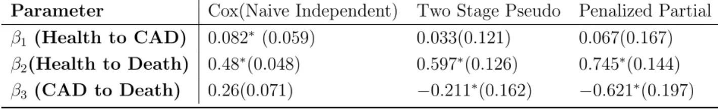
3.4 Data Application Result:Estimation of Gender Effect in Time to CAD
with Death as a Semi-competing Risk . . . 73
4.1 Bivariate Survival Data with a Semicompeting Risk Simulation Result:
σ2
b=0.1/0.5; Sample size=100 . . . 102
4.2 Bivariate Survival Data with a Semicompeting Risk Simulation Result:
σb=0.1/0.5 sample size=200 . . . 103
4.3 Baseline Age, Mean and Median Age of Event Onset By Gender . . 107
4.4 Application result for gender effect in CAD and Depression with death
as semi-competing risk . . . 108
6.1 Clayton Copula Estimation Approach with Data Generated From
Clay-ton Copula with Exponential Distribution as Marginal . . . 115
6.2 Two-stage Semiparametric Estimation Approach with Data Generated
From Clayton Copula with Exponential Distribution Marginal . . . 116
6.3 Pseudo Partial Likelihood Estimation Approach with Data Generated
LIST OF FIGURES
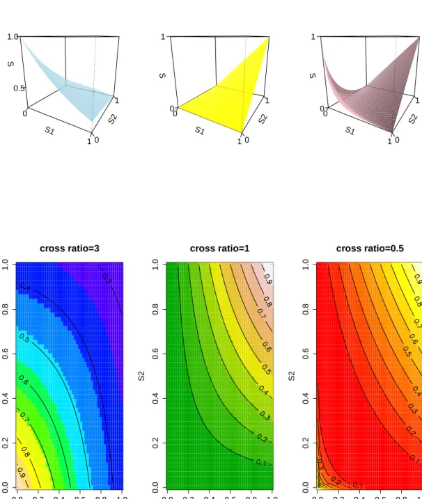
2.1 The Joint Distribution of Bivariate Survival Model Plot under Varying
Cross Ratio: the first row is the 3-D plot, the height represents joint
survival probability and the marginal of survival distribution ofT1 and
T2 are identical; the second row is the contour plot, the number on the
black line represent the value of joint survival probability . . . 16
2.2 Cumulative Hazard Plot of Two Diseases by Gender Group: The first
row is the cumulative hazard of time to CAD by Male and Female group respectively, the red line represents depression group, the back line is non-depression group; the second row is the cumulative hazard of time to depression by Male and Female group respectively, the red
line is CAD group and black line is Non-CAD group. . . 36
3.1 Two events with a Semi-competing Risk . . . 49
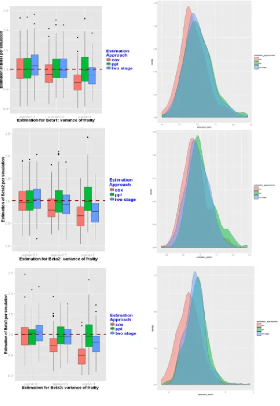
3.2 Simulation Results for the Normal Frailty Scenario Presented in Box
Vixen Plot and Empirical Distribution Plot.The red dash line
repre-sents the true parameter. . . 68
3.3 Simulation Results for the Log-Normal Frailty Scenario Presented in
Box Vixen Plot and Empirical Distribution Plot.The red dash line
represents the true parameter. . . 69
3.4 Survival plots of time to CAD, time to death, time to death in the CAD
group and time from CAD to death, by gender, the red line represented
4.1 Two Non-terminal Events and a Terminal Event as Semi-competing
Risk . . . 77
4.2 Hazard by Each Pathway with Frailty Model Setup in Bivariate Time
to Events Data with Semi-competing Risk . . . 87
4.3 The Summarization of Possible Pathway in Bivariate Time to Events
Data with a Semi-competing Risk . . . 88
4.4 The Multi-state Flow Chart to Composite Joint Likelihood for
Bivari-ate Time to Events with a Semi-competing Risk . . . 88
4.5 The Transition Plot for Component for Nelson-Aalen Estimator in
Multi-state Model From State i to State j . . . 89
4.6 Data Preparation Flaw Chart for Simulation Study: Generating
Bi-variate Time to Events Data with a Semi-competing Risk . . . 100
4.7 IIDP data for CAD and depression bivariate time to event with a
Chapter 1
Introduction
1.1 Overview
This dissertation is devoted to develop new methodologies in survival analysis of joint models of bivariate time to events data with a semi-competing risk. This research work is primarily motivated by some interesting problem emerging from observational study of chronic diseases in aging cohort, in which a better understanding of chronic diseases natural history is needed to better understand and identify risk factor, to learn diseases relations, to design better health care and intervention for optimal treatment.The data support through out this dissertation come from electronic med-ical records (EMRs) in a longitudinal cohort of elderly African Americans enrolled in the Indianapolis-Ibadan Dementia Project (IIDP)(Hendrie et al., 2001).
Multivariate survival data arises when one encounters the situation of corre-lated multiple types of events including the same type of events observed from siblings or multiple events experienced by the same individual. A naive approach analyzing these survival data separately for each survival outcome by ignoring the association among the multiple events may produce biased results. Furthermore, investigating on how these multiple events relate to each other may offer important information on the underlying mechanisms for these events. In this dissertation, we focus on the joint modeling of bivariate time to event data with the estimation of the association parameters and also in the situation of a semi-competing risk.
By studying and reviewing some current and well established techniques in survival analysis realm, the proportional hazards model, proposed by Cox (1972), is certainly one of the most widely, used and studied regression model for time-to-event data, the cox model focus on exploring the relationship between the baseline hazard and treatment effect with the adjustment for the other explanatory variables. Extend from cox model, in order to take into account the heterogeneity due to the unobserved risk factor, Clayton (1978) and Vaupel et al. (1979) proposed to use frailty model or mixed proportional hazards model. The frailty term which can be understand as random effects, if these effects are subject-specific and unobserved heterogeneity stands for overdispersion and the model is called univariate frailty model (Wienke, 2010). In the case when random effects are shared by groups of subjects, a clustering effect is there, i.e. observations belonging to the same group are dependent. This is the case of shared frailty models (Hougaard, 2012).
The integration of frailty and multi-event models can provide powerful survival models to study the risk of many interrelated events while accounting for dependence among multiple events. Many practical situations can be thought of in which such integration is of interest. The main problem motivating our research arises from ob-servational study of elder cohort, in which the participant usually was facing multiple diseases due to aging. Thus, we need to take into account the dependence between events when we conduct analysis and make inference .
The dissertation contains three related topics on bivariate time to event mod-els. The first topic is on estimating the association parameter between bivariate survival functions. The second is on semiparametric pseudo-likelihood and semi-parametric penalized partial likelihood models of univariate time to event with a
semi-competing risk. The third part is on semiparametric models of bivariate times to event with a semi-competing risk.
1.2 Covariate Dependent Cross Ratio of Bivariate Survival Times
Most current methods used in estimating the association parameter in bivariate time to event data have used either the copula approach or a frailty approach where the association parameter is treated as a constant parameter or as a nuisance. Cross-ratio is an association parameter which measures the dependence structure between two correlated failure times. One advantage of using cross-ratio as a dependence measure is that it has an attractive hazard ratio interpretation by comparing two groups of interest. In shared frailty models for bivariate survival data the frailty is identifiable through the cross ratio function, which provides a convenient measure of association for correlated survival variables. The cross ratio function may be used to compare patterns of dependence across models and data sets.
To estimate the cross ratio as a function, Nan et al. (2006) partitioned the sample space of the bivaratiate survival time into rectangular regions with edges par-allel to the time axes and assumed that the cross ratio is constant in each retangular region. Shih and Louis (1995) and Shih and Albert (2010) proposed a two stage semiparametric likelihood based method to estimate constant cross ratio and piece-wise cross ratio under competing risk setup, respectively. In the context of compet-ing risks and nonparametric appraoches,Cheng and Fine (2008), Bandeen-Roche and Ning (2008)and Ning and Bandeen-Roche (2014) proposed a nonparametric method for estimating the piecewise constant time-varying cause-specific cross ratio using the binned survival data based on the same partitioning idea for the sample space,
counted the concurrence events pair and discordinate events pair can formed up a logistics-form of regression procedure for the estimation procedure. Recent years, Li and Lin (2012), Othus and Li (2010) and Hsu and Moodie (2007) characterized the dependence of bivariate survival data through the correlation coefficient of normally transformed bivariate survival times. Such methods, however, require assumptions of specific copula models for the joint survival function, for which appropriate model checking techniques are lacking.
Hu et al. (2011) proposed an estimation approach for time dependent cross ratio using a pseudo-partial likelihood approach. Build on Hu et al. (2011)’s method-ology, we propose a cross ratio set-up which allows the modeling of covariate effects on the association parameter. The advantage of such a model is that covariate effect is linked with cross ratio explicitly. In addition, the non-parametric estimation ap-proach does not require the specification of either the joint or the marginal survival functions and thus is robust against model misspecification. A simulation study is conducted to evaluate the estimation performance of this nonparametric estimation approaches. The proposed estimation approach is used to estimate gender effects on the association between time to coronary artery disease (CAD) and time to depression using data from an elderly cohort.
1.3 Frailty based Semiparametric Models for Time to Event Data with a
Semi-competing Risk
Semi-competing risk often arises in biomedical research, in particular, in studies of aging when individuals at risk of a particular disease die from other causes. As the two-types of events are usually correlated, models for semi-competing risks should
properly take account of the dependence. In the literature, copula models are popular approaches for modeling of such data. However, the copula model postulates latent failure times and marginal distributions for the non-terminal event that may not be easily interpretable in reality. Further, the development of regression models is complicated for copula models. To overcome these issues, the well-known illness-death models have been recently proposed for more flexible modeling of semi-competing risks data.
In the second part of this dissertation, we proposed a frailty model approach for a survival outcome with a semi-competing risk. The standard likelihood based ap-proach for multivariate lognormal frailty models involves multi-dimensional integrals over the distribution of the multivariate frailties, which almost always do not have analytical solutions. Numerical solutions such as Gaussian quadrature rules, Monte Carlo sampling have been routinely used in literature.However, as the dimension in-creases, these approaches still remain computationally demanding.
In order to retain the nice interpretation of frailty model and overcome the computational challenge, two estimation approaches are proposed and compared. The first is a two-stage pseudo-likelihood approach where cumulative baseline hazards were first estimated by a nonparametric method. Parameter estimation is then achieved by maximizing the pseudo-likelihood functions where the estimated cumulative hazards from stage one were used. In the second approach, we propose a penalized partial likelihood function for parameter estimation and inference similarly to the concept
used in the Cox's partial likelihood. An estimation procedure based on penalized
pseudo-partial likelihood is used for estimating covariate effects. The penalized partial likelihood is obtained by Laplace approximation to the true likelihood. Penalized
Cox PH model discussed by Gray (1992); Perperoglou (2014) provided methods of parameter estimation. A simulation study is conducted to compare the estimation performance of these two approaches. The proposed estimation approach is used to estimate gender effects on the time to coronary artery disease (CAD) with time to death as a semi-competing risk.
1.4 Frailty-based Multi-event Semiparametric Models for Failure Time
Data with Semi-competing Risks
The third topic of this dissertation extends the models considered in the second part to bivariate survival outcomes with a semi-competing risk.
In medical research, multi-event and multi-stage data arises when a individual was at risk of multiple disease, or a certain disease progressed in several states. It was crucial to study the inner structure and dependence between multiple diseases or multiple states.
In this part, we propose to use frailty based semparametric model introduc-ing random effects to account for unobserved risk factors, possibly shared by multi-ple diseases or multimulti-ple states. For model estimation, we developed and evaluated parametric, two stage semiparametric estimation and penalized partial likelihood ap-proach.The two stage pseudo-likelihood approach and the penalized pseudo-partial likelihood approach are also be used and compared in simulation studies.
In many epidemiological studies of the elderly population, it has been ob-served that individuals at risk of one chronic condition tend to have increased risk of other medical conditions with a substantial numbers having multiple chronic condi-tions. Studying the co-occurrence of these conditions may identify common biological
pathways linking these disorders and ultimately lead to effective treatment and pre-vention strategies. Another complication facing the studies in aging is death due to other causes which can be indirectly related to the conditions under study through genetic or environmental exposures related to the individual’s susceptibility to both disease and death. The proposed approaches were applied to data from the elderly cohort to determine risk factors associated with CAD (Coronary Artery Disease) and depression with death as the semi-competing risk.
1.5 Main Contribution and Structure of Dissertation
The work presented in this thesis contributes to research in survival analysis in follow-ing areas: modelfollow-ing methodology and data applications, and simulation techniques.
The main contribution to modeling methodology consists of proposing co-variate dependent cross ratio estimation methods, and frailty based semiparametric model in the presence of semi-competing risk data. Up to now, there existed no co-variate dependent association measure for bico-variate time to event data. Capturing the dependent structure between multiple survival events is a challenging topic. Our proposed cross ratio model offered a feasible approach to measure the dependence between bivariate survival times. In addition, we propose to use frailty based model approach to handle semi-competing risk data and multiple event, which captures the transition between multiple events and also account for informative censoring caused by the other event and death.
Two estimation approaches have been developed and investigated in the dis-sertation: a parametric and a semiparametric approach. First, fully parametric infer-ence, based on maximum marginal likelihood, is considered. Then, a semiparametric
estimation approach, based on maximum penalized partial likelihood, is proposed and investigated(Rotolo and Legrand, 2012; Rotolo et al., 2013).
Another contribution of our work is that we developed a general method in multi-event research for simulating data according to a given scenario. Dependence can be added between time variables of grouped subjects, to study the effect of cluster-ing. Moreover, the simulation method is able to introduce, using copulas, dependence between times of different transitions while fixing the marginal distributions accord-ing to a given scenario. This is a useful tool to study, for instance, the robustness of (frailty) multi-event models .
The structure of this dissertation is as follows. In Chapter 2, we focus on the estimation of dependent association parameter: cross ratio between bivariate survival times. In Chapter 3, we present two estimation approaches for semi-competing risk models. In Chapter 4, we extent the semi-competing risk model presented in chapter 3 to bivariate time to event data. Chapter 5 gives concluding marks.
Chapter 2
Covariate Dependent Cross Ratio of Bivariate Survival Times
2.1 Abstract
Cross ratio is formed as the ratio of two conditional hazard rates for one events given the other event. Inherited the nice interpretation of hazard ratio from survival analysis setup, cross ratio can be interpreted as hazard ratio of one event conditional the status of the other event. It is very meaningful to investigate the covariate effect on the cross ratio, which can be a useful tool to explain contribution of the certain component to the dependent between two time to events. In this paper, first, we extended two methodologies in constant cross ratio estimation into covariate adjust cross ratio with multiplicative covariate effect set up, which are Clayton copula model and Shih and Louis(1995) two stage semiparametric model. Then, we conducted a simulation study comparing Hu et al. (2011)’s non-parametric estimator with parametric estimator from copula approach and semi-parametric estimator from Shih and Louis (1995)’s two stage approach. In the mean time, we presented a comprehensive review and discussion of these three methodologies. To illustrate three estimation methodologies, we analyzed data from Indianapolis-Ibadan Dementia Project (IIDP) to investigate the gender effect between cardiovascular event and depression.
2.2 Introduction
Bivariate survival outcomes are often collected in medical studies. In many cases, the two failure times may be correlated. Earlier interests have focused on determin-ing the correlations between disease occurrence times of family members in genetic epidemiology such as the age of onsets to asthma or type I diabetes in twin studies (Hyttinen et al., 2003; Thomsen et al., 2011). However, there is also an increasing interest in examining times to two related diseases observed from the same individ-ual in order to identify common pathways and potential risk factors underlying both diseases. For instance, there have been considerable research efforts focusing on the link between coronary artery disease (CAD) and depression. CAD and depression are both common in late life and have been shown to be associated with increased risk of disability and mortality(Callahan et al., 1998). A “vascular depression hy-pothesis” was first proposed by Alexopoulos et al. (1997) when the authors proposed that cardiovascular disease may predispose, precipitate, or perpetuate some geriatric depressive syndromes. However, the vascular depression hypothesis was recently re-placed by a new model describing the association between CAD and depression as the outcome of ”two intertwined, mutually reinforcing disorders”(de Jonge and Roest, 2012).Evidence supporting this new bi-directional model between CAD and depres-sion includes the increased risk of CAD in people suffering from depresdepres-sion and that late-life depression has been found to be associated with neuroimaging findings for subclinical cerebrovascular disease(de Groot et al., 2000; Hawkins et al., 2014). A gender difference in CAD and comorbid depression has been observed prompting a search for a common immunological basis including the role of inflammation in both
diseases (M¨oller-Leimk¨uhler, 2010; Wright et al., 2014). Therefore, analysis of bi-variate survival outcomes includes estimating the dependence between the two times to events and determining the contributions from common risk factors as the two primary objectives.
The dependence between two survival times has been discussed previously in the literature (Diva et al., 2008; Li and Lin, 2012; Li et al., 2008; Rondeau et al.,
2012) . One naive approach is to use global rank measures such as Kendall’s τ and
Spearman’s coefficientρ(Hougaard, 2012; Kendall, 1948). However, two major issues
were not addressed using these estimators: first, both estimators cannot incorporate censoring information leading to potentially biased and inefficient estimates; second, both estimators do not account for covariate contribution to the association of the two event times.
In contrast to the global rank based association measures, cross ratios, for-mulated as the ratio of two conditional hazard functions, offer a direct measure of dependence between two survival times that can account for censoring and accom-modate potential covariates(Kalbfleisch and Prentice, 2002). There are three broad classes of estimation approaches for cross ratio estimation.
The first is a full parametric approach. Clayton (1978) introduced the Clay-ton copula model as an explicit closed-form bivariate survival function model with a constant cross ratio. Oakes (1982) demonstrated that the Clayton copula model can be derived using a frailty framework, where a common latent variable induces a correlation between events. A parametric approach will require the specification of a bivariate survival model, such as the Clayton model, and the simultaneous estima-tion of the marginal survival funcestima-tions and the cross ratio parameter. The second
is a semi-parametric approach developed by Shih and Louis (1995). The marginal survival functions were first estimated by Kaplan-Meier estimators and used in the bivariate survival function to derive the cross ratio estimate. Shih and Louis (1995) showed that the two stage semi-parametric approach is efficient when the marginal survival functions were unknown. Lawless and Yilmaz (2011) compared a one stage semiparametric maximum likelihood (ML) approach and a two stage semi-parametric pseudo maximum likelihood (PML) approach for the Clayton model and Frank cop-ula. In the one stage semi-parametric ML approach, the marginal functions, and the association parameter were estimated using non-parametric methods simultaneously. Lawless and Yilmaz (2011) concluded that that the two-stage semi-parametric PML was the preferable approach for marginal distribution estimation in most situations that do not involve covariates. When covariates were presented in the marginal dis-tributions, however, the one stage ML method can be substantially better in some settings. When the bivariate survival model is misspecified, Lawless and Yilmaz (2011) showed that the two stage PML can perform worse than the one stage ML for cross ratio estimates. They also pointed out that one stage semiparametric approach was more computationally intensive compare to two stage method.
Both the parametric and the semi-parametric approaches assume a constant cross ratio.Nan et al. (2006) considered a piece-constant cross ratio set up by parti-tioning the sample space of bivariate survival function into rectangles each of which was assumed to have a constant cross ratio. Hu et al. (2011) proposed a nonparamet-ric estimation approach which allowed cross ratio to be modeled as a time varying function. For estimation, Hu et al. (2011) constructed an objective function by mim-icking the partial likelihood in the David (1972) propertional hazard model.
No previously published studies have considered modeling covariate effect in the cross ratio. Given the interpretation of cross ratio as a conditional hazard ratio for one event given the other event, It will be interesting to determine the effect of covariates on the cross ratio in order to account for the change in the association between two events. In this paper, we extend Clayton (1978) ’s copula model and Shih and Louis (1995)’s two stage semiparametric model into covariate adjusted cross ratio setup with multiplicative covariate effect similar to Hu et al. (2011). We present a simulation study comparing Hu et al. (2011) ’s non-parametric estimator with the parametric estimator from the copula approach and a two stage semi-parametric estimator from Shih and Louis (1995). The proposed method is illustrated using data from the Indianapolis-Ibadan Dementia Project (IIDP) to determine gender effect on the associating between time to coronary artery disease (CAD) and time to depression (Gao et al., 1998; Hendrie et al., 2001; Unverzagt et al., 2001).
In the following sections, we present the notations and model set up in Section 2. We describe estimation approaches in Section 3 and results from a simulation study in Section 4. We present results from the IIDP data analysis in Section 5 and conclude the article with a discussion in Section 6.
2.3 Notation, Definition and Model Setup
In this section, we introduce some common notation and definition in survival analysis and cross ratio analysis
Consider a pair of correlated continuous failure times (T1, T2) that are subject
to right censoring by a pair of censoring times (C1, C2). Let (S1, S2) and (f1, f2)
respec-tively. Let (h1, h2) and (H1, H2) denote the corresponding marginal hazard and cu-mulative hazard, respectively. We assume that censoring times are independent of
failure times. Suppose we observe n independent and identically distributed vectors
of (X1, X2,∆1,∆2) , where X1 = min(T1, C1), X2 = min(T2, C2),∆1 = I(T1 ≤ C1)
and ∆2 =I(T2 ≤C2). Here I(·) denotes the indicator function. We further assume
that there are no ties among the two observed times.
Cross ratio function of T1 and T2 at time (t1, t2) is defined as
α(t1, t2) = h2(t2|T1 =t1) h2(t2|T1 > t1) = h1(t1|T2 =t2) h1(t1|T2 > t2) (2.1)
The function can be interpreted as the ratio of the hazard rate of the conditional
distribution of T1, given T2, to that of T1. givenT2 ≥t2.(Oakes, 1989) We have
h(t1|T2 =t2) =− ∂1S1(t1|T2 =t2) S1(t1|T2 =t2) =−∂1,2S(t1, t2) ∂2S(t1, t2) and h(t1|T2 ≥t2) =− ∂1S(t1, t2) S(t1, t2) Then, α(t1, t2) = ∂1,2S(t1, t2)×S(t1, t2) ∂1S(t1, t2)×∂2S(t1, t2) = f(t1, t2)×S(t1, t2) ∂1S(t1, t2)×∂2S(t1, t2)
Where, ∂1f(t1, t2) = ∂f(t1, t2) ∂t1 ∂2f(t1, t2) = ∂f(t1, t2) ∂t2 ∂1,2f(t1, t2) = ∂f(t1, t2) ∂t1∂t2 f(t1, t2) is a function of t1 and t2.
When α(t1, t2) = 1, the two events are independent; when α(t1, t2) > 1, the
two events are positively correlated; whenα(t1, t2)<1, the two events are negatively
correlated. Hu et al. (2011); Oakes (1982, 1986, 1989) Figure (2.1) demonstrate the joint survival distribution of bivariate survival model under different cross ratio using
perspective 3D surface plot and 2D contour plot. Whencrossratio= 3, the two time
to event were positively correlated, the joint survival will increase as two marginal survival increase, the contour plot (Figure (2.1) bottom left) showed concave feature. Whencrossratio= 1, the two events were independent, the joint survival is the direct
product of two marginal survival S = S1(t)·S2(t). When crossratio = 0.5, the two
events were negatively correlated, the joint survival showed twisted structure over the space.
Let W be a set of covariates. Cross ratio function conditional on covariates
can be defined as:
α(t1, t2;w) = h2(t2|T1 =t1, W =w) h2(t2|T1 > t1, W =w) = h1(t1|T2 =t2, W =w) h1(t1|T2 > t2, W =w) (2.2)
Figure 2.1: The Joint Distribution of Bivariate Survival Model Plot under Varying Cross Ratio: the first row is the 3-D plot, the height represents joint survival
proba-bility and the marginal of survival distribution of T1 and T2 are identical; the second
row is the contour plot, the number on the black line represent the value of joint survival probability S1 0 1 S2 0 1 S 0.5 1.0 cross ratio=3 S1 0 1 S2 0 1 S 0 1 cross ratio=1 S1 0 1 S2 0 1 S 0 1 cross ratio=0.5 0.0 0.2 0.4 0.6 0.8 1.0 0.0 0.2 0.4 0.6 0.8 1.0 cross ratio=3 S1 S2 0.0 0.2 0.4 0.6 0.8 1.0 0.0 0.2 0.4 0.6 0.8 1.0 cross ratio=1 S1 S2 0.0 0.2 0.4 0.6 0.8 1.0 0.0 0.2 0.4 0.6 0.8 1.0 cross ratio=0.5 S1 S2
Here, we further assume that the covariateW has a multiplicative effect on the cross ratio:
α(β;t1, t2) =α(β;t1, t2,w) = α0(t1, t2)·exp(w·β) (2.3)
where α0(t1, t2) is the cross ratio for a reference value defined by w, and exp(w·β)
is an exponential function of w. For example, if W = 0 is to be used as a reference
for the effect ofW, then
α0(t1, t2) = h2(t2|T1 =t1, W = 0) h2(t2|T1 > t1, W = 0) = h1(t1|T2 =t2, W = 0) h1(t1|T2 > t2, W = 0) (2.4)
Model (2.3) effectively separates the reference cross ratio function and the covariate effect thus providing an opportunity to model each piece separately.
2.4 Estimation Approaches
In this section, we describe three estimation approaches. The first two approaches are based on the parametric formation of Clayton copula. Thus, these two approaches can only accommodate discrete covariates in order to achieve constant cross ratio within each level of the covariate thus retaining the Clayton copula form. The third approach is nonparametric following the spirit of (Hu et al., 2011) where both discrete and continuous covariates can be handled(Hu, 2011).
2.4.1 Bivariate Clayton Copula Approach
The definition of cross ratio (2.1) is equivalent to the following second-order partial differential equation: ∂2−log(S(t1, t2)) ∂t1∂t2 + (α(β;t1, t2)−1)∂−log(S(t1, t2)) ∂t1 ∂−log(S(t1, t2)) ∂t2 = 0 (2.5)
where S(t1, t2) is the joint survival function of (T1, T2) at (t1, t2).
When α(β;t1, t2) = α is constant, it can be shown that equation (2.5) has a
unique solution of the form
Cα(t1, t2) = [S1(t1)−(α−1)+S2(t2)−(α−1)−1]−
1
α−1 (2.6)
where Cα(t1, t2) is called Clayton copula (Clayton, 1978). The formation of Clayton
copula is differed by the value of cross ratio α.
Cα(t1, t2) = [S1(t1)−(α−1)+S2(t2)−(α−1)−1] − 1 α−1 α >1 S1(t1)·S2(t2) α= 1 max([S1(t1)−(α−1)+S2(t2)−(α−1)−1]−α−11,0) α <1
where S1 and S2 are the marginal survival functions of T1 and T2.
Clayton Copula and Archimedean Family
In fact the Clayton copula belongs to an important family of copulas known as Archimedean copulas which have a simple form with a variety of dependence
struc-tures. The copula function C is generally define as multivariate function which can couples the joint survival function to its univariate margins in a manner completely analogous to the way in which a copula connects the joint distribution function to its margins. (Nelsen, 2007) The support of copula approach is supported by Sklar’s canonical representation theorem.
Theorem 1 (Sklar’s Canonical Representation) Let S be an N-dimensional
survival function with margins S1, . . . , SN. Then, S has a copula representation:
S(t1, . . . , tN) = C(S1(t1), . . . , SN(tN))
The copula C is unique if the margins are continuous.
Archimedean copula model has the following representation:
H(u, v) =φ−1(φ(u) +φ(v)), (u, v)∈[0,1]2
where φ : [0,1]→[0,+∞] is a function satisfying φ(1) = 0, φ(0) =∞, φ0(x)<0 and
φ00(x)>0. Then H(u, v) is a distribution function on[0,1]2 with uniform marginals.
Commonly used Archimedean copula models include:
• Clayton copula, whereφ(u, α) =u−(α−1)−1,
• Frank copula, where φ(u, θ) = log11−−θθu,
Parametric Clayton Copula Likelihood
The joint likelihood of bivariate time to events data can be written as
L=Y
i
f(t1, t2)δ1·δ2·−S12(t1, t2)δ1·(1−δ2)·−S21(t1, t2)(1−δ1)·δ2·S(t1, t2)(1−δ1)·(1−δ2) (2.7)
where S(t1, t2)is the joint survival function and
S12(t1, t2) = ∂S(t1, t2) ∂t1 (2.8) S21(t1, t2) = ∂S(t1, t2) ∂t2 (2.9) f(t1, t2) = ∂ 2S(t 1, t2) ∂t1∂t2 (2.10)
Under the Clayton copula structure. The likelihood can be written as
Li =f(ti1, ti2)∆i1∆i2 ·[− ∂Cα(β;t1,t2)(ti1, ti2) ∂ti1 ]∆i1(1−∆i2) ×[−∂Cα(β;t1,t2)(ti1, ti2) ∂ti2 ](1−∆i1)∆i2·C α(β;t1,t2)(ti1, ti2) (1−∆i1)(1−∆i2) (2.11)
Based on (2.6) and ∂S∂t(t) =−h(t)·S(t), we have
By symmetry, ∂Cα(β;t1,t2)(t1, t2) ∂t2 (2.12) =−S(t1, t2)· {S1(t1)−(α(β;t1,t2)−1)+S2(t2)−(α(β;t1,t2)−1) −1}−1 ·S2(t2)−(α(β;t1,t2)−1)·h2(t2)
Then ∂Cα(β;t1,t2)(t1, t2) ∂t1 (2.13) =−{S1(t1)−(α(β;t1,t2)−1)+S2(t2)−(α(β;t1,t2)−1)−1} − 1 α(β;t1,t2)−1−1 ·S1(t1)−(α(β;t1,t2)−1)·h1(t1) =−S(t1, t2)· {S1(t1)−(α(β;t1,t2)−1)+S2(t2)−(α(β;t1,t2)−1)−1}−1 ·S1(t1)−(α(β;t1,t2)−1)·h1(t1) f(t1, t2) = ∂2C α(β;t1,t2)(t1, t2) ∂t1∂t2 (2.14) = (1 +α(β;t1, t2))·h1(t1)·S1(t1)−(α(β;t1,t2)−1) · {S1(t1)−(α(β;t1,t2)−1)+S2(t2)−(α(β;t1,t2)−1)−1}−α(β;t11,t2)−1−2 ·h2(t2)·S2(t2)−(α(β;t1,t2)−1)
The joint likelihood for all the observation isL=Qn
i=1Li. Letφ = (γ1
0,γ
20,β),
where γ10,γ20 are the parameters in the marginal survival distribution S1(t1) and
S2(t2)), respectively. β is the parameter for the covariate in the cross ratio function.
Uγ10(φ), Uγ20(φ), Uβ(φ) are the score functions which are essentially the first
deriva-tive of the log of (2.11) forγ10,γ20,β. Maximum likelihood estimate ˆφ is the solution
to Uγ10(φ) = 0, Uγ20(φ) = 0, Uβ(φ) = 0. Under Cox and Hinkley (1979) regularity
variance-covariance matrix I−1, where I is the information matrix obtained from the second derivative of likelihood equation (2.11)(Cox and Oakes, 1984). Given full para-metric functions of the marginal survival functions, maximum likelihood estimates of
β as well as parameters in the marginal survival functions can be obtained.
2.4.2 Two Stage Semiparametric Estimation Approach
In the parametric approach described above, the two marginal survival functions are assumed to be fully specified and the joint survival model follows a Clayton copula. In a two-stage semiparametric estimation approach, the marginal survival functions
are estimated by the nonparametric Kaplan-Meier approach as ˆS1 and ˆS2 first. The
cross ratio parameter, ˆβ, is then estimated at the second stage by maximizing the
pseudolikelihood function L( ˆS1,Sˆ2,β).
Write (ui, vi) for the non parametric estimator of (S1(X1i), S2(X2i)). Then
given (ui, vi), j = 1, . . . , n, the likelihood of β is
Lpseudo(β, ui, vi) = Y i fα(β;t1,t2)(ui, vi) ∆1i·∆2i ·∂Cα(β;t1,t2)(ui, vi) ∂ui ∆1i·(1−∆2i) ·∂Cα(β;t1,t2)(ui, vi) ∂vi (1−∆1i)·∆2i ·Cα(β;t1,t2)(ui, vi) (1−∆1i)·(1−∆2i) (2.15) where C(u, v;α(β;t1, t2)) ={u−(α(β;t1,t2)−1)+v−(α(β;t1,t2)−1)−1} −α(β;t1 1,t2)−1 (2.16) ∂C ∂u ={u −(α(β;t1,t2)−1)+v−(α(β;t1,t2)−1)−1}−α(β;t11,t2)−1−1·u−(α(β;t1,t2)−1)−1 (2.17)
∂C ∂v ={u −(α(β;t1,t2)−1)+v−(α(β;t1,t2)−1)−1}−(α(β;t1,t2)−1)−1 ·v− 1 α(β;t1,t2)−1−1 (2.18) ∂2C ∂u∂v =(1 + 1 α(β;t1, t2)−1 ){u−(α(β;t1,t2)−1)+v−(α(β;t1,t2)−1)−1}−(α(β;t1,t2)−1)−2 (2.19) ·u−(α(β;t1,t2)−1)−1·v−(α(β;t1,t2)−1)−1
Letl(β, S1, S2) be the log likelihood function in equation (4.8) andU(β, S1, S2)
the score function of β, then
U(β,Sˆ1,Sˆ2) =
∂l(β,S1,ˆ S2ˆ)
∂β (2.20)
The pseudo likelihood estimator β? is the solution to score function.
To estimate standard error, we extend the results from Theorem 2 in Shih and Louis (1995) by chain rule of derivation.We use the notation from Shih and Louis
(1995). Let cross ratio α be a function of covariate of interest β, i.e. α(β). Then,
according to chain rule, we have
Wβ = ∂l(α(β;t1, t2), u, v) ∂β = ∂l(α(β;t1, t2), u, v) ∂α(β;t1, t2) · ∂α(β;t1, t2) ∂β (2.21) Vβ = ∂2l(α(β;t 1, t2), u, v) ∂β2 = ∂ 2l(α(β;t 1, t2), u, v) ∂α(β;t1, t2)2 ·( ∂α(β;t1, t2) ∂β ) 2+ ∂l(α(β;t1, t2), u, v) ∂α · ∂2α(β;t 1, t2) ∂β2 Vβ,1 = ∂l(α(β;t1, t2), u, v) ∂β∂u = ∂l(α(β;t1, t2), u, v) ∂α(β;t1, t2)∂u · ∂α(β;t1, t2) ∂β Vβ,2 = ∂l(α(β;t1, t2), u, v) ∂β∂v = ∂l(α(β;t1, t2), u, v) ∂α(β;t1, t2)∂v · ∂α(β;t1, t2) ∂β
The estimator for standard error can be expressed as ˆ τ = τˆ 2 1 + ˆτ22 ˆ τ4 1 , (2.22) where ˆτ2
1 is the model based variance estimator and can be obtained from the second
derivative of pseudo likelihood
ˆ τ12 = 1 2 n X i=1 −Vβ(β?,Sˆ1(X1i, X2i)), ˆ τ22 = 1 n n X i=1 [ ˆI1(X1i,∆1i,β?) + ˆI2(X2i,∆2i,β?)]2 where ˆ I1(X1k, δ1k,β?) = 1 n X k Vβ,1(β?,Sˆ1(X1k, X2k)) ˆI10(X1k, δ1k)(X1k), ˆ I2(X2k, δ2k,β?) = 1 n X k Vβ,2(β?,Sˆ1(X1k, X2k)) ˆI20(X2k, δ2k)(X2k) and ˆ I10(X1i, δ1i)(X1k) = −Sˆ1(X1k){ IX1i ≤X1k,∆1i = 1 ˆ p1i − X X1l≤X1i,X1k ∆ ˆΛ1(X1l) ˆ p1l }, ˆ I20(X2i, δ2i)(X2k) = −Sˆ2(X2k){ IX2i ≤X2k,∆2i = 1 ˆ p2i − X X2l≤X2i,X2k ∆ ˆΛ2(X2l) ˆ p2l }
∆ ˆΛi(t) is a Nelson’s estimator, which can be calculated as ∆ ˆΛi(t) = I
{Y¯i(t)>0}
¯
Yi(t) d ¯ Ni(t),
where ¯Yi(t) = PjI{Xij ≥ t} and Ni(t) = PjNij(t). β? is the solution for score
equation in (2.20). Shih and Louis (1995) showed that if cross ratioα(β;t1, t2) = αis
2.4.3 Nonparametric Pseudo-Partial Likelihood Estimation Approach
The nonparametric approach from Hu et al. (2011) is motivated by the Cox propor-tional hazards model, which is use to capture the local feature of the dependence structure (Hu, 2011). The idea is to group observations into distinct strata by co-variate values, then using one survival time as exposure and using the other survival time as the outcome in order to construct a pseudo-partial likelihood function.
The procedure to construct the pseudo partial likelihood followed the in-terpretation of conditional hazard ratio in epidemiology terminology. If we treat {j : T1j = t1} and {j : T1j > t1} as“exposure” and“non-exposure” groups,
respec-tively, then from (2.2) , the cross ratio can be interpreted as the hazard ratio of T2
between these two groups within the stratum W =w. Given t1 = X1i, by
mimick-ing the partial likelihood used in the Cox’s models, Hu et al. (2011) proposed the following pseudo-partial likelihood function:
n Y j=1 [ h2(X2j|X1j =X1i,wj =wi) I(X1j=X1i) P X2k≥X2jI(X1k≥X1i)h2(X2j|X1j =X1i,wj =wi) I(X1k=X1i)] I(X1j≥X1i)∆2j∆1i (2.23) n Y j=1 [ h2(X2j|X1j > X1i,wj =wi)·α(X1i, X2j,wj) I(X1j=X1i) P X2k≥X2jI(X1k≥X1i)h2(X2j|X1j > X1i,wj =wi)·α(X1i, X2j,wj) I(X1k=X1i)] Iij (2.24)
Where Iij =I(X1j ≥X1i)∆2j∆1i. With some simplification, the above equation can
be write as n Y j=1 [ α(X1i, X2j,wj) I(X1j=X1i) P X2k≥X2jI(X1k ≥X1i)α(X1i, X2j,wj) I(X1k=X1i)] I(X1j≥X1i)∆2j∆1i (2.25)
Denote (4.9) asL(1)i . Considering the symmetric structure of the definition of θ(t1, t2, w), given t2 =X2i, we have : L(2)i = n Y j=1 [ α(X2i, X1j,wj) I(X2j=X2i) P X1k≥X1jI(X2k ≥X2i)α(X2i, X1j,wj) I(X2k=X2i)] I(X2j≥X2i)∆1j∆2i (2.26)
The finial pseudo-partial likelihood function can be obtained, by multiplying these two objective functions from all subjects,
Ln= n
Y
i=1
L(1)i ·L(2)i (2.27)
The estimator obtained by maximizing (3.28) is then called the pseudo-partial likeli-hood estimator.
Hu et al.(2011) proved that, under some regularity conditions, the maximum
pseudo-partial likelihood estimator β have n12( ˆβ −β) converges in distribution to
a normal random variable with mean zero and variance I(β)−1Σ(β)I(β)−1, where
I(β) = 2E(∆1 ·∆2 ·w2) and Σ(β) is the asymptotic variance for Un(β) = ∂log∂βLn,
which can be estimated using sample variance.
For continuous covariates, the observation with ”relative close” covariate value can be combined into the same ”group”. This can be achieved by replacing the
indicator functionI(Wj =Wi) by a kernel function Kh(Wj−Wi) in (4.9) and (4.10).
2.5 Simulation Study
We conducted a simulation study to evaluate the performance of these three estima-tion approaches under covariate dependent cross ratio setup. Since simulating data
from a bivariate distribution with an arbitrary cross ratio function is most possible because there may not be a corresponding closed form survival function, we simulated data from a Clayton model with piecewise constant cross ratio following Nan et al. (2006). This simulation setup had also been used in He and Lawless (2003).
Two simulation scenarios were considered, the first scenario was used to demon-strate the performance of each estimation approach under model is correctly specified and with identical marginal distribution; the second scenario was used to demon-strate the performance of each estimation approach under model is misspecified. For
all three scenarios both equal and unequal censoring percentage of T1 and T2 were
considered.
2.5.1 Data Setup
Bivariate data (T1i, T2i),i= 1, . . . , n,were generated one component at a time. First,
T1i was generated from the uniform variate ui1 ∼U[0,1] by
Ti1 = [
−log(ui1) λ1
]p11 (2.28)
Then, Ti2 was generated from the independent variate ui2 ∼U[0,1] by
Ti2 = [ 1 −(αi(β;t1, t2)−1) ·log(1−u 1−αi(β;t1,t2) i1 +u 1−αi(β;t1,t2) i1 ·u − αi(β;t1,t2) αi(β;t1,t2)−1 i2 ) λ2 ]p12 (2.29)
In our simulation study, the cross ratio function was setup asαi(β;t1, t2) = α0·
exp(β·wi) andα0 = 3 andβ = 0.5, and we usedwi ∼Bernoulli(0.5). We considered
times Ci1 and Ci2 were generated independently from uniform distributions.C ∼ U nif orm(0,4.8) orC ∼U nif orm(0,4.1), with probability of censoring 10% or 30%,
respectively. For each scenario, we generated 1000 simulate samples; sizes n = 100,
n= 400 and n = 800 were considered.
For each estimation approach, we calculated relative bias, standard error esti-mate, and the estimated coverage probability rates of 95% confidence intervals using the asymptotic normal distribution assumption for each of the estimates. The relative bias were calculated as the difference between estimates and true value divided by
the true value, βˆ−ββ.
2.5.2 Simulation Results when the Model is Correctly Specified
Table (2.1) summarized the simulation results for model is correctly specified scenario, the relative bias, model based standard error, empirical standard error of paramet-ric Clayton copula approach, semiparametparamet-ric two stage approach and nonparametparamet-ric pseudo partial likelihood estimators of the association are given. The data was gen-erated from Clayton copula with two levels of cross ratio and identical exponential distribution as marginal survival. The marginal survival were generated from
iden-tical exponential distribution, Si(t) = exp(−t), where i = 1,2. And the true value
of β was 0.5. The Table (2.1) presented the results for equal percentage censoring
scenario and unbalanced censoring senior.
For no censoring case, the bias of parametric Clayton copula estimates was the smallest among three estimation approach, this results was as expected since the data were generated from Clayton copula and Clayton copula estimation approach can revival all the information in the simulated data by using correct likelihood. We
also found that, as expected, the bias and error estimates were decreasing as sample size increasing for all three estimates.
When censoring percentages were equal, the bias and error estimates were increasing as censoring percentage increasing. We also found that under moderate percentage of censoring Clayton copula approach performed adequately well, but if the censoring percentage were considerable, the performance of Clayton copula ap-proach was not ideal compare to two stage semiparametric apap-proach and nonparamet-ric pseudo partial likelihood approach. And the two stage semiparametic estimates and non-parametric pseudo partial likelihood estimates performed more robust results against censoring compare to Clayton copula approach. But among three estimates, the nonparametric pseudo partial likelihood(PPL) estimates had smallest inflamma-tion percentage of the bias, which indicated that the non parametric PPL estimate was the most robust estimates against censoring.
In unbalanced censoring scenario, we found that nonparametric PPL estimates was the most robust and accurate estimate among three estimates. Both parametric Clayton copula estimate and semiparametric two stage estimate approach were very sensitive to unbalanced censoring scenario. Especially, the performance of these two estimates were quite poor if the censoring percentage was quite different between two event, this drawback may resulted by using the Clayton copula structure during the estimation for these two approaches, since both parametric Clayton copula approach and semiparametric two stage approach were highly relied on Clayton copula struc-ture. From the likelihood formula in (2.11), the unbalanced censoring won’t influence
much on the joint survival S(t1, t2) = Cα(t1, t2), but the ∂S∂t(t11,t2) = ∂Cα∂t(t11,t2) and
∂S(t1,t2)
∂t2 =
∂Cα(t1,t2)
T able 2.1: Sim ulation Result for Co v ariate De p enden t Cross Ratio Estimation with Correctly Sp ecified Mo del S cenario: Marginal Surviv al of T1 and T2 are Exp onen tial Di str ibution, the true β = 0 . 5 P arametric(Cla yton Copula ) Semiparametric(Tw o Stage) Nonp arametric(Pseudo P artial Lik eliho o d) T1 T2 R .B ias β M .S Eβ E .S Eβ M .C Pβ R .B ias β M .S Eβ E .S Eβ M .C Pβ R .B ias β M .S Eβ E .S Eβ M .C Pβ sample size=100 0 censor 0 censor 0.034 0.185 0.177 0.95 -0.019 0.171 0.1 95 0.96 0.064 0.17 3 0.169 0.93 10% censor 10% censor 0.063 0.203 0.216 0.92 -0.009 0.184 0.2 11 0.94 0.087 0.22 4 0.219 0.93 30% censor 30% censor 0.056 0.244 0.251 0.95 0.10 9 0.239 0.238 0.92 0.146 0.530 0.5 18 0.9 0 censor 10% censor 0.054 0.195 0.190 0.94 -0.097 0.180 0.2 09 0.94 0.082 0.19 9 0.195 0.94 10% censor 30% censor 0.052 0.234 0.238 0.92 -0.115 0.213 0.2 34 0.96 0.100 0.37 3 0.385 0.97 30% censor 0 censor 0.066 0.231 0.239 0.92 0.02 9 0.207 0.216 0.96 0.109 0.347 0.3 49 0.95 sample size=400 0 censor 0 censor 0.001 0.091 0.100 0.93 -0.029 0.086 0.0 82 0.96 0.026 0.07 8 0.078 0.95 10% censor 10% censor 0.032 0.100 0.105 0.92 0.01 6 0.097 0.087 0.92 0.039 0.101 0.1 20 0.96 30% censor 30% censor -0.043 0.12 1 0.129 0.97 0.127 0.195 0.114 0.76 0.046 0.242 0.237 0.93 0 censor 10% censor 0.014 0.096 0.101 0.94 -0.060 0.106 0.0 88 0.88 0.032 0.08 9 0.087 0.95 10% censor 30% censor 0.012 0.116 0.132 0.91 -0.036 0.134 0.1 05 0.84 0.051 0.17 2 0.169 0.92 30% censor 0 censor -0.018 0.11 4 0.122 0.94 -0.099 0.131 0.102 0.86 0.03 9 0.159 0.156 0.9 sample size=800 0 censor 0 censor 0.013 0.064 0.064 0.95 -0.028 0.057 0.0 73 0.88 0.001 0.05 3 0.054 0.96 10% censor 10% censor 0.044 0.071 0.074 0.92 -0.021 0.061 0.0 79 0.86 0.014 0.06 9 0.068 0.94 30% censor 30% censor -0.011 0.08 6 0.086 0.95 0.032 0.080 0.101 0.88 0.028 0.165 0.161 0.93 0 censor 10% censor 0.030 0.068 0.066 0.97 -0.129 0.062 0.0 78 0.72 0.006 0.06 1 0.060 0.93 10% censor 30% censor 0.022 0.082 0.076 0.97 -0.117 0.074 0.1 00 0.78 0.022 0.11 8 0.115 0.94 30% censor 0 censor 0.026 0.081 0.087 0.91 -0.137 0.072 0.0 82 0.8 0.017 0.108 0.106 0.95 R.Bias: Relativ e bias M.SE: Mo del based standard error. E.SE: Empirical sta ndard error. M.CP: 95 % co v erage probabilit y based on M.SE.
2.5.3 Simulation Results when the Model is Misspecified
Table (2.2) summarized the simulation results for model is misspecified specified, the relative bias, model based standard error, empirical standard error of paramet-ric Clayton copula approach, semiparametparamet-ric two stage approach and nonparametparamet-ric pseudo partial likelihood estimators of the association are given.The data were gen-erated from Clayton copula model with Weibull distribution as identical marginal,
Si(t) = exp(−2·t
1
3), where i= 1,2.
From the Table (2.2), we found that the compare to the semiparametric two stage estimate and nonparametric PPL estimate, the Clayton copula estimate was more sensitive to the structure of the marginal survival. If the marginal is misspec-ified, the estimate from Clayton copula approach performed poorly compare to the others. The two stage estimation was much less affected by the misspecification of the marginal model in contrast to the parametric approach, since in semiparametric two stage approach, the marginal distributions were estimated in the first stage us-ing nonparametric estimates, so it can handle the misspecification of marginal in the first stage and lead to a relative accurate cross ratio estimate in the second stage. The nonparametric pseudo partial likelihood approach provides superior and robust estimation compare to the other two approaches, since the nonparametric approach was not rely on the information of marginal distribution.
T able 2.2: Sim ulation Result for Co v ariate Dep enden t Cross Ratio Estima tion with Mis-sp ecified Mo del Scenario: Marginal Surviv al: Margina l Surviv al of T1 and T2 are W eibull Distribution with λ = 2 ,p = 3, the true β = 0 . 5. P arametric(Cla yton Copula ) Semiparametric(Tw o Stage) Nonp arametric(Pseudo P artial Lik eliho o d) T1 T2 R .B ias β M .S Eβ E .S Eβ M .C Pβ R .B ias β M .S Eβ E .S Eβ M .C Pβ R .B ias β M .S Eβ E .S Eβ M .C Pβ sample size=100 0 censor 0 censor -0.241 0.16 5 0.183 0.83 -0.087 0.170 0.215 0.9 0.060 0.172 0. 170 0.93 10% censor 10% censor -0.246 0.17 6 0.197 0.87 -0.090 0.184 0.230 0.88 0.07 1 0.209 0.207 0.94 30% censor 30% censor -0.156 0.23 4 0.392 0.9 -0.172 0.250 0.260 0.98 0.105 0.494 0. 488 0.93 0 censor 10% censor -0.243 0.17 0 0.189 0.85 -0.108 0.176 0.248 0.84 0.07 4 0.191 0.189 0.92 10% censor 30% censor -0.255 0.20 2 0.202 0.88 -0.306 0.216 0.268 0.82 0.06 8 0.324 0.340 0.96 30% censor 0 censor -0.231 0.19 7 0.228 0.86 -0.418 0.208 0.261 0.72 0.08 0 0.296 0.292 0.91 sample size=400 0 censor 0 censor -0.284 0.08 2 0.093 0.55 -0.054 0.082 0.072 0.96 0.02 6 0.077 0.078 0.95 10% censor 10% censor -0.285 0.08 7 0.098 0.58 -0.045 0.087 0.075 0.96 0.03 6 0.094 0.093 0.93 30% censor 30% censor -0.275 0.11 4 0.121 0.75 0.070 0.113 0.143 0.9 0.06 3 0.220 0.218 0.94 0 censor 10% censor -0.282 0.08 5 0.094 0.58 -0.093 0.086 0.084 0.94 0.02 9 0.085 0.084 0.93 10% censor 30% censor -0.277 0.10 0 0.113 0.66 -0.307 0.111 0.125 0.6 0.063 0.146 0. 144 0.92 30% censor 0 censor -0.302 0.09 7 0.101 0.62 -0.401 0.104 0.108 0.56 0.03 0 0.132 0.131 0.92 sample size=800 0 censor 0 censor -0.298 0.05 8 0.059 0.28 -0.085 0.186 0.186 0.96 0.00 1 0.053 0.054 0.96 10% censor 10% censor -0.293 0.06 1 0.061 0.31 -0.119 0.200 0.212 0.88 0.00 9 0.064 0.064 0.93 30% censor 30% censor -0.260 0.08 1 0.082 0.63 -0.109 0.270 0.289 0.96 0.03 7 0.150 0.148 0.93 0 censor 10% censor -0.297 0.06 0 0.058 0.3 -0.101 0.192 0.210 0.92 0.006 0.058 0. 058 0.92 10% censor 30% censor -0.287 0.07 0 0.068 0.44 -0.259 0.234 0.306 0.84 0.01 7 0.099 0.099 0.95 30% censor 0 censor -0.285 0.06 8 0.072 0.46 -0.333 0.227 0.258 0.82 0.01 2 0.091 0.091 0.95 R.Bias: Relativ e bias M.SE: Mo del based standard error. E.SE: Empirical sta ndard error. M.CP: 95 % co v erage probabilit y based on M.SE.
2.6 Data Application: Estimate Gender Effect in Cross Ratio between Time to CAD and Depression
In this section, we demonstrate our proposed method in real data application example.
2.6.1 Indianapolis-Ibadan African American Cohort
To illustrate the three estimation approaches in covariate dependent cross ratios, we present a data analysis exploring potential gender differences in the association be-tween time to coronary artery disease (CAD) and time to depression using data from the Indianapolis-Ibadan Dementia Project (IIDP). The Indianapolis-Ibadan demen-tia project (IIDP) was a 20 year National Institute on Aging funded a longitudinal study of dementia and its risk factors in elderly community-dwelling African Ameri-cans living in Indianapolis, Indiana and elderly community-dwelling Yoruba living in Ibadan, Nigeria. Recently, data from the African-American participants in the study were merged with data from the Indiana Network for Patient Care, a regional health information exchange, allowing us to examine medical conditions such as CAD and depression, using electronic medical records(EMR) obtained in the routine care of older adults.
For our analysis, the study population consisted of African American partici-pants of the IIDP. All were age 65 or older residing in Indianapolis, Indiana. Recruit-ment was conducted at two-time points. During the first recruitRecruit-ment in 1992, 2212 African Americans age 65 or older living in Indianapolis were enrolled in the study. In 2001, the project enrolled 1893 additional African American community-dwelling participants 70 years and older. All participants agreed to undergo regular follow-up
cognitive assessment and clinical evaluations. Details on the assembling of the orig-inal cohort and the enrichment cohort were described elsewhere.Hall et al. (2009); Hendrie et al. (2001) Electronic medical records from 1992 to December 31, 2014, were retrieved as a re-identified data set to examine cardiovascular diseases and other risk factors. There were 4105 participants enrolled. After excluding 854 participants who did not have EMR and 28 participants who had CAD or depression before en-rollment, there were 3223 participants free of CAD and depression at baseline. Mean age at baseline was 75.6 (standard deviation=6.38) and 68.04 % were women. In Table 2.3 we present the number of participants with incident CAD, depression and both events by gender. Female participants had a higher percentage of depression events and male participant have a higher percentage of CAD events, in addition, the female participants had higher percentages of experience both depression and CAD events compare to male group. Figure (2.2) is the survival plot of CAD event and depression by gender group, from which we can see that the two events are somewhat correlated and there is a slight difference by gender.
Table 2.3: Demographic Characteristic of IIDP Data with Number of Event and Incidence Rate by Each Gender Group
Gender Total CAD Depression CAD and Depression
Female 2192 822 (37.5%) 479 (21.85%) 193 (9.55%)
Male 1031 396(38.4%) 138 (13.38%) 62 (6.01%)
Total 3223 1191(36.95%) 617(19.14%) 271(8.4%)
In Table 2.4, we present the median age for each disease onset by gender and the status of the other disease. For the male group, we found that participants who had one disease had an earlier onset of the other disease. However, female participants
with depression actually had a slightly later onset of CAD while female participants with CAD had the similar age of onset for depression as those without CAD. The Figure 2.2 is the cumulative hazard plot for time one disease onset give the other disease status for each gender. From Figure 2.2, we observed that the male group tend to have more close association compare to female group. This result showed that there maybe gender difference in the association between the two diseases. Table 2.4: Median Age Onset for Each Disease by Gender and the Status of the Other Disease
CAD Depression
Total Female Male Total Female Male
Total 79.01 80.21 79.03 Total 80.23 80.06 80.4
Depression 80.19 80.89 76.39 CAD 80.48 81.05 79.81
No Depression 79.58 79.94 79.2 No CAD 79.01 78.91 81.05
CAD: Cardiovascular event DP: Depression
2.6.2 Estimate Gender Effect in Cross Ratio between Time to CAD and
Depression
Denote tCAD as time to CAD andtDP as time to depression; M as male group andF
as female group; hCAD(·) as hazard for CAD and hDP as hazard for depression. To
estimate the cross ratio as a function of gender, we use following multiplicative model
θ(tCAD, tDP;Gender=M) =
hDP(tDP|TCAD =tCAD, Gender=M)
hDP(tDP|TCAD > tCAD, Gender=M)
= hCAD(tCAD|TDP =tDP, Gender=M) hCAD(tCAD|TDP > tDP, Gender=M)
Figure 2.2: Cumulative Hazard Plot of Two Diseases by Gender Group: The first row is the cumulative hazard of time to CAD by Male and Female group respectively, the red line represents depression group, the back line is non-depression group; the second row is the cumulative hazard of time to depression by Male and Female group respectively, the red line is CAD group and black line is Non-CAD group.
70 80 90 100 0.0 0.2 0.4 0.6 0.8 1.0 1.2
Time to CAD for Male
Cumulative Hazard Non-Depression Depression 70 80 90 100 0.0 0.5 1.0 1.5
Time to CAD for Female
Cumulative Hazard Non-Depression Depression 70 80 90 100 0.0 0.1 0.2 0.3 0.4
Time to Depression for Male
Cumulative Hazard Non-CAD CAD 70 80 90 100 0.0 0.2 0.4 0.6 0.8
Time to Depression for Female
Cumulative Hazard
Non-CAD CAD
and
θ(tCAD, tDP;Gender=M) =θ0(tCAD, tDP;I(Genderi =F))·exp(I(Genderi =M)·β)
(2.31)
whereI(Genderi =M)is an indicator function for male andθ0(t1, t2;I(Genderi =F))
is the reference cross-ratio in females, i.e.
θ0(tCAD, tDP;I(Genderi =F)) =
hDP(tDP|TCAD =tCAD, Gender=F)
hDP(tDP|TCAD > tCAD, Gender=F)
= hCAD(tCAD|TDP =tDP, Gender=F) hCAD(tCAD|TDP > tDP, Gender=F)
(2.32)
Where M indicate male andF indicate female.
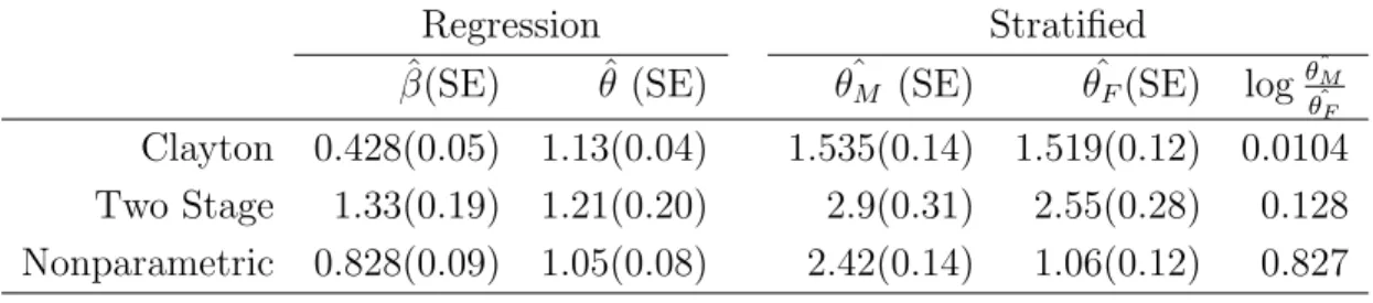
Three estimation approaches were used in this data set. Results were presented in Table 2.5. All three estimation approaches showed the estimated cross ratio larger than 1 in the reference group indicating that women who had early onset of one disease
were more likely to have an onset of the other disease. The coefficientβ for the gender
indicator variable in equation (2.31 ) was estimated to be greater than 0 suggesting that the association between the two disease onsets is stronger in males than the association in females, but this difference is not statistically significant. In order to verify these results, we also conducted stratified analyzes by estimating constant cross
ratio in each gender group separately. In Table 2.5, θcF and θcM represent the cross
ratio estimation for each group. All three approaches still showed greater cross ratio estimate in male participants than in female participants. However, only log-ratio of the two nonparametric cross ratio estimates of male over the female was close to the coefficient estimate produced using the nonparametric approach. Both parametric