Predicting the Effects of Missense Variation on Protein Structure, Function, and Evolution

(1)

Predicting the Effects of

Missense Variation on Protein

Structure, Function, and Evolution

The Harvard community has made this

article openly available.

Please share

how

this access benefits you. Your story matters

Citation

Jordan, Daniel Michael. 2015. Predicting the Effects of Missense

Variation on Protein Structure, Function, and Evolution. Doctoral

dissertation, Harvard University, Graduate School of Arts &

Sciences.

Citable link

http://nrs.harvard.edu/urn-3:HUL.InstRepos:17464216

Terms of Use

This article was downloaded from Harvard University’s DASH

repository, and is made available under the terms and conditions

applicable to Other Posted Material, as set forth at

http://

nrs.harvard.edu/urn-3:HUL.InstRepos:dash.current.terms-of-use#LAA

(2)

Predicting the Effects of Missense Variants

on Protein Structure, Function, and

Evolution

a dissertation presented by

Daniel Michael Jordan to

The Committee on Higher Degrees in Biophysics in partial fulfillment of the requirements

for the degree of Doctor of Philosophy in the subject of Biophysics Harvard University Cambridge, Massachusetts April 2015

(3)

(4)

Thesis advisor: Professor Shamil R. Sunyaev Daniel Michael Jordan

Predicting the Effects of Missense Variants on Protein

Structure, Function, and Evolution

Abstract

Estimating the effects of missense mutations is a problem with many important applications in a variety of fields, including medical genetics, evolutionary theory, population genetics, and protein structure and design. Many popular methods exist to solve this problem, the most widely used of which are PolyPhen-2 and SIFT. These methods, along with most other popular methods, rely on multiple sequence alignments of orthologous protein sequences. Based on the amino acids observed in each column of the alignment, they produce a profile describing how tolerated each amino acid is at each position. They then compare the wild-type and variant amino acids to this profile to pro-duce a prediction.

In practice, these methods are fast, robust, and relatively reliable. However, from a theoretical perspective, they have at least three significant shortcomings:

1. They use effects on selection as a proxy for effects on phenotype and protein structure and function.

2. They treat each position as independent, ruling out most forms of interactions between sites. 3. They do not explicitly model the process of evolution, instead assuming that sequences we

observe more or less represent an equilibrium state.

With the recent explosion of sequencing technology, as well as the steady increase of computational power, we are now beginning to have enough data to investigate these simplifications and see how much they really affect the performance of these methods.

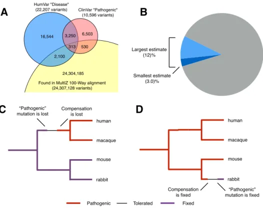
In this dissertation, I present three such investigations. First, I describe a modified predictor de-signed to predict risk for a specific disease, hypertrophic cardiomyopathy (HCM), rather than gen-eral seletive effect. This method achieves significantly higher accuracy than methods without such specific domain knowledge. Next, I describe a model of pairwise interactions between sites, demon-strating both statistically and within vivoevidence that approximately 7–12% of disease-causing variants may be mispredicted by these methods due to such interactions. Finally, I describe a hybrid method that uses an alignment-based estimator to inform a parametric model of evolution, resulting in a small but significant improvement in accuracy.

(5)

Acknowledgments

It is a bit of a cliché to say that grad school was a difficult journey, but it is undoubtedly true. It has taken its toll — on my bank account, on my mental and physical health, and on my relation-ships. Still, over the past seven (seven!) years I have done a lot of work of which I am very proud, much of which is contained in this document, and, more importantly, learned and grown a great deal, both scientifically and personally. There are many people I must thank for making that possi-ble.

Thanks to Jim Hogle and Michele Jakoulov, for running the least soul-sucking Ph.D. program I have ever heard of; my advisor, Shamil Sunyaev, for his wide-ranging expertise and faintly hubris-tic attitude towards science; and Ivan Adzhubey, who spent many hours fixing things I broke and tolerated my attempts to improve on his software.

Thanks to all the professors who have sat on my various committees, namely, Steve Blacklow, Leonid Mirny, Eugene Shakhnovich, Kricket Seidman, Mike Desai, Jun Liu, and Cynthia Morton; to my collaborators at the LMM: Sam Baxter, Matt Lebo, Birgit Funke, and Heidi Rehm; and at Duke: Stephan Frangakis, Erica Davis, and Nico Katsanis.

Thanks to my scientific mentors from the before times, without whom I never would have gotten here: Laurel Harmon, Erik Zuiderweg, Bob Koeppe, Martin Philbert, Doug Stone, and, going all the way back to middle school, Tim Wilson.

Thanks to all the members of the Sunyaev Lab past and present, and especially Chris Cassa and Dan Balick, for many hours of useful conversation and advice and many more of useless conversa-tion and whiskey.

Thanks to Brandy Freitas, my drinking buddy, co-TF, and all around comrade-in-arms in the Biophysics program; and to Julia Liu, Sophie Zaaijer, Amy Xu, and David Ferrero, my crack team of scientist-musicians, who were instrumental (ha ha) to maintaining my sanity.

Thanks to Adam Becker and Vlad Barash, who blazed the trail to the Ph.D. for me and always had a sympathetic ear for grad school frustrations; and to my sometime girlfriend Rachel Carpman, who was a source of great strength for many years, and remains one of my best cheerleaders.

Finally, my deepest thanks and love to my parents Lawrence and Elizabeth Jordan and my brother Jonathan Jordan, from whom I have never felt a lack of love and pride; and my dear, dear friends Max Gladstone, Stephanie Neely, and Marshall Weir, who have loved and supported me uncondi-tionally for the last seven years.

(8)

0

Introduction

0.1 Motivation

In recent years, deep sequencing of genomes and exomes has begun to take the place of traditional association studies as the method of choice for probing the landscape of human variation. The growth of next-generation sequencing has brought with it an explosion of rare variants, with ev-ery newly sequenced individual carrying hundreds of never-before-seen coding variants38,141,179.

(9)

Confidently assigning functional or phenotypic significance to these variants is a very difficult task. Traditional human genetics methods involving observation in multiple individuals with the same phenotype are not usually feasible for these extremely rare variants. In some genes, as many as half of all known variants are intractible to traditional genetic evidence and considered to have “unknown significance,” either due to the variant not having been observed in a large enough sample of indi-viduals or due to the lack of appropriate race-matched controls for these observations153. On a small scale, such as for an individual patient, these unknown variants can be addressed within vivoorin vitrofunctional testing. However, it remains unfeasible to apply these experiments to the thousands of variants observed by a large clinical lab or the hundreds of thousands of variants observed in a population-level sequencing study.

To fill this gap, a large and growing collection ofin silicomethods to predict the effects of variants has emerged over the last decade and a half34,101,144. These methods have seen a great deal of use in a variety of applications, including prioritization of candidate variants and genes, characterization of fitness effects of variants on a population level, and diagnosis of rare Mendelian disorders4,7,179. However, these tools are still generally seen as immature, and are often compared unfavorably to functional analysis and human genetic evidence71,153,176,205. One important reason for this is that the accuracy of these methods remains fairly low, and the groups that produce them systematically over-estimate the accuracy of their own methods, resulting in a reputation for unreliability72,183. Another is that the databases containing variants of “known” effect used to train these predictors are pol-luted with dubious annotations, which both affects the accuracy of the predictors themselves and contributes to the perception that computational methods are unreliable27,111.

As whole-exome and whole-genome sequencing become more and more common, the number of variants in need of interpretation is only going to increase, and the need for accurate and trusted tools for variant interpretation is only going to become more acute. Improving the reliability and reputation of these tools and addressing their quirks and faulty assumptions is essential for the

(10)

fu-ture of the field.

0.2 The Method

Evolution can be seen as one enormousin vivoexperiment for evaluating the effects of amino acid changes. Changes are proposed by a stochastic mutation process, and those with negative effects on fitness are rejected by natural selection. Thus the history of evolution contains an enormous amount of information about which changes are tolerated and which are not. We can access part of this history using comparative genomics, by comparing sequences from different species. The oldest and most widely used variant effect prediction methods, SIFT and PolyPhen, have relied on this insight since their introduction in 2001142,172, and most widely-used methods continue to do so to this day101.

In general, the fixation or loss of an allele is controlled by the strength of selection against that allele. To be precise, the probability of fixationπ1of an allele with frequencypis

π1(p) = 1−e −2Nesp

1−e−2Nes (1)

wheresis the strength of selection against the allele*andNeis the effective population size†67. If

selection is sufficiently strong (Nes ≫ 1), the allele is deterministically lost; alleles with such strong

selection acting against them should never be found fixed in any species. On the other end of the spectrum, if selection is sufficiently weak (Nes ≪ 1), genetic drift overcomes selection against the

*_{Note that for the purposes of this discussion, and indeed through the bulk of this dissertation, I am}

ig-noring positive selection. There are tools to detect positive selection, but for the most part positive selection is irrelevant to the problem of variant effect prediction, as alleles under sufficiently strong positive selection fix very rapidly and are unlikely to be found as variants requiring interpretation.

†_{I won’t go into the exact theoretical definition of}_N

e, but in most cases it can roughly be thought of as

the minimum population size at the last population bottleneck. In this case we are not really talking about a single population, but rather a pool of many different populations over the history of evolution. Based on the effective population sizes measured for existing vertebrate species, we can probably assume thatNefor these

(11)

allele, and the allele can become fixed stochastically with probabilitypjust as though it were neutral. According to this principle, any allele that is seen to be fixed in any species can be assumed to have only weak selection acting against it.

Even at the most basic level, this principle is remarkably useful for predicting the effects of alleles and the relative importance of sites. For example, suppose we implement the following extremely simple classifier: any allele observed in another species in our multiple sequence alignment (in this case we will use the MultiZ whole-genome orthologous alignment of 100 vertebrate species103) is benign, and any allele never observed is pathogenic. Using the HumVar dataset, a dataset of variant annotations based on the SwissVar database and commonly used for training and testing variant effect predictors22,139, this extremely simple classifier correctly predicts 91% of pathogenic variants and 63% of benign99. This should be considered a baseline for many more advanced prediction algorithms; in some sense, the further refinements made by methods like PolyPhen and SIFT only serve to address the 37% of benign variants that are mispredicted by this simple method‡.

The difference between this method and the basic framework used by methods like SIFT and PolyPhen is that these methods move from the yes-or-no question of “is this amino acid tolerated at this site?” to the concept of a “profile” of amino acid preferences at each site. Moving from a more-preferred amino acid to a less-more-preferred one is likely to be damaging, while moving in the opposite direction is probably not. The way we typically think about this profile is as the distribution of amino acids likely to be found at the site. It’s often referred to as the equilibrium distribution of amino acids, based on the idea that evolution is a stochastic process that we are sampling from when we observe sequences. If the process is at equilibrium, the amino acids we observe should be drawn from this equilibrium distribution. The most naive way of computing this distribution is simply to count up the number of observations of each amino acid — e.g. if there is a position where we

ob-‡_{The 9% of pathogenic variants that are mispredicted by this simple method turn out to be much harder}

to deal with. They will be discussed in greater detail below; Chapter 2 of this dissertation is aimed at character-izing these variants.

(12)

serve 15 sequences with valine, 4 with isoleucine, and 1 with tryptophan, we would naively describe the preference of this amino acid site as 75% valine, 20% isoleucine, and 5% tryptophan.

There are additional adjustments that are commonly made on top of this naive method. One very commonly used adjustment is to add pseudocounts to account for the chemical properties of amino acids and our prior expectations about the variability of sites80. For example, in our valine-isoleucine-tryptophan example, we might observe that tryptophan is very chemically different from valine and isoleucine, and its presence therefore suggests that the site is probably somewhat tolerant of a wide variety of different amino acids. Our method might add pseudocounts of other non-observed amino acids to account for this variability. We might also observe that leucine is very chemically similar to valine and isoleucine, and if these two amino acids are both tolerated leucine probably is as well. We could therefore add pseudocounts of leucine to account for the fact that our observations of valine and isoleucine represent implied observations of leucine. Another adjustment is to weight sequences based on their relatedness171. This is based on the insight that two very closely related sequences carrying the same amino acid are not really two independent observations of that amino acid, since they are sampled from the same branch of the evolutionary tree.

This profile must then be converted to a prediction. The amino acid profile of a site is a 19-dimensional vector§, but a prediction of pathogenicity should ideally be a one-dimensional value. Some methods use a simple statistical model to make the conversion; for example, SIFT142simply reports the expected frequency of the variant amino acid, while PANTHER-PSEC180reports the log likelihood ratio of the wild-type and variant amino acids. Others, such as PolyPhen-22and SNAP18, use the frequencies from the profile as features in various machine learning classifiers. This approach also allows explicit incorporation of other features, such as sequence context, secondary structure elements, or geometric features extracted from solved 3D structures. In fact, most such methods

§_{There are 20 different amino acid types, but the requirement that the frequencies sum to 1 restricts the}

(13)

also incorporate some additional information of this kind. Even with the addition of these features, though, the amino acid tolerance extracted from the multiple sequence alignment remains the most informative predictive feature for all predictors that use it.

Many variations exist on this basic method, using different methods for retrieving sequences and constructing alignments, different models to extract and adjust profiles, different sources of addi-tional annotation, different machine learning methods, and different training datasets of known variants. However, the basic method of using the profile of amino acids observed in evolutionary history to estimate the amino acid tolerance of a given site is still widely used today, 14 years after the release of the original PolyPhen and SIFT methods. Even the latest state-of-the-art methods still use these profile scores as major components of their predictors25,108. It may seem strange that there has been no major improvement on this method, considering that it is completely agnostic about bio-logical function and protein structure, which should both be vitally important to determining the strength of selection. Though many methods incorporate features intended to capture these factors, these features rarely add much information on top of the profile score. This information seems al-ready to be encoded in the profile score. After all, in some sense the profile of observed amino acid frequencies is the result of integrating this information throughout the history of evolution.

0.3 Issues

Careful readers of the above may notice a number of places where I have hand-waved away im-portant distinctions or discarded large swaths of established theory. This is not entirely due to my own lack of care. There are a few important issues that most modern methods systematically ignore. Three of these issues will motivate the three subsequent chapters of this dissertation:

(14)

0.3.1 Deleterious vs. Pathogenic

One area where the field as a whole lacks clarity is the question of what, exactly, these tools are de-signed to predict. Common use cases, including most of those mentioned above and most of those proposed by the authors of these methods, primarily focus on predictingphenotypes, especially med-ically relevant phenotypes. However, what these methods really measure isselection. In general prin-ciple, selection is not necessarily a good proxy for phenotypic effect. There are many severe and med-ically relevant phenotypes that may not produce very large selective effects, such as those with late onset, reduced penetrance, or pleiotropic effects on selection198,208. Conversely, there are many mild or medically irrelevant phenotypes that nevertheless produce large selective effects. For example, a sperm motility defect causing a∼10% reduction in fertility should appear extremely deleterious, despite having minimal noticeable effect on the individual’s health.

This conflation obviously has the potential to influence the accuracy of predictions, and it has consistently been remarked on across the entire history of variant effect prediction, from the origi-nal paper reporting the PolyPhen method (“only a small fraction of deleterious amino-acid altering SNPs …lead to total loss of function of the affected protein, and the rest must have relatively mild ef-fects”)172to the paper reporting the CADD method published last year (“it is at present not possible to precisely calibrate the relationship between …estimated deleteriousness and the likelihood that a variant is pathogenic”)108. Nevertheless, most people who use or design these methods do not pay much attention to this problem, since the predictions do, after all, work reasonably well. Undoubt-edly they could work better if they made an effort to account for the relationship between selection and pathogenicity, but it’s unclear how much better. Additionally, accounting for this relationship probably requires a great deal of domain knowledge about specific genes and phenotypes, and may not be possible on a genome-wide level.

(15)

0.3.2 Independence of Sites

It seems reasonable enough to claim that evolution explores the range of allowed amino acids at every site, and that we can reconstruct that range by looking at the sequences output by evolution. However, hidden within this formulation is the tacit assumption that the range of allowed amino acids is defined site-by-site, and that each site has a fundamentally independent profile of amino acid preferences. In fact, the massivein vivoexperiment of evolution does not just produce legal lists of amino acids, but instead legal protein sequences, each of which folds into a three-dimensional structure and carries out its function as a complete sequence. The two concepts are only equivalent if interactions between sites have minimal biological importance, and the effect of multiple variants together is almost always the sum of their individual effects. There is ample evidence in modern genetics that interactions between sites do exist and are important, though there is some debate over how common they really are in the history of evolution6,16,36,130.

The specific worry for variant effect prediction methods is that a nonhuman sequence might con-tain a specific amino acid that would be pathogenic in the context of the human sequence, but is observed in a context that compensates for its pathogenic effect. In this case, a prediction method would be likely to incorrectly predict the variant as benign, because in fact it is observed in nature as a benign variant. This situation, where a variant that causes a disease in human is fixed in an-other species, is often referred to as a compensated pathogenic deviation (CPD). Several studies have observed and commented on this phenomenon, frequently also observing that roughly 10% of fixed differences between species are pathogenic to one of the species30,112,115. However, despite this relatively frequent occurrence, prediction methods generally do not make an effort to account for CPDs. This is generally because there is no way to knowa prioriwhich interactions are impor-tant for compensation. Without specific biological or biochemical knowledge about the protein in question, the relevant compensation could be any position or combination of positions in the entire

(16)

genome.

0.3.3 Parametric Methods

The idea that sequences are samples from a stochastic process of evolution is not unique to these prediction methods; in fact, it’s a very common way of viewing evolution. There is a large and well-developed set of models that treats evolution as a branching continuous-time Markov process92. These models explicitly account for the tree structure of relationships between sequences. They also can in priniciple explicitly account for differences and similarities between amino acids, accepting as parameters both the relative frequencies of different amino acids and the rates of substitution be-tween them. It may then seem odd that variant effect prediction methods do not use these state-of-the-art models, preferring to use the heuristic methods of sequence weighting and pseudocounts¶. In fact, there are some methods that do use these models, the most widely-used of which are phy-loP154and GERP++41. They are referred to as “parametric” methods, because they deal with the rate parameters of these models, as opposed to the profile methods, which do not have parameters in the same sense. These methods are often used to identify funcitonal sites and conserved elements, especially in noncoding regions4,34,79. However, they are generally not as accurate as profile-based methods for amino acid substitutions52,108, and therefore are not as widely used in coding sequences.

It is somewhat frustrating that parametric methods don’t perform better, since they should in some sense be more correct than profile methods. Especially in cases where reasonably trustworthy phylogenetic trees exist, such as for whole-genome orthologous alignments where we in principle know the relationships of the species, it seems like we are throwing data away by not explicitly mod-eling these trees. One easy explanation for why these methods don’t work as well is that they are estimating the wrong quantity: instead of the profile of tolerated amino acids at a site, they esti-¶_{These methods are “heuristic” in the sense that they ignore features of the theoretically correct model}

(17)

mate the rate of evolution at the site. This rate parameter should be a good indicator of evolutionary constraint, but it does make some amount of sense that the higher-dimensional amino acid pro-file might contain more information than a single rate score per site. In principle, it is possible to represent the equilibrium distribution of amino acids in a parametric method — indeed, any such method must deal with this distribution on some level, because it is a feature of the model. The re-sults produced tend not to be too useful, though. Based on my experience experimenting with these models, there appear to be two reasons for this:

1. It is very difficult to deal with the full 20-letter amino acid alphabet in a fully parametric way. It requires a 20×20 substitution rate matrix with 380 independent parameters, far too many to reasonably infer using the 100-sequence orthologous alignments we typically have access to, not to mention the seconds per site or less of computational time we typically have in large-scale prediction tasks.

2. The likelihood surface of the 19-dimensional amino acid frequency vector seems to be very flat. If there are two amino acids that are both clearly tolerated, it is very difficult to say what the “correct” values for their relative preferences are. Is it 50%–50%? 80%–20%? 20%–80%? Profile methods can safely ignore the differences between these scenarios; parametric meth-ods can’t, because they have a dramatic influence on parameter values. In a likelihood surface that is high-dimensional and lacks a sharp peak, likelihood methods can easily get stuck in local maxima or fail to collect enough information to overcome the prior.

In the course of my doctoral studies, I have investigated these and other concerns about vari-ant effect prediction methods, with the hope of pointing the way towards improvements in these already well-established methods. The following chapters represent the results of three research projects aimed at addressing the three specific issues described above.

(18)

But wait: let us question a holy man, a prophet, even a man skilled with dreams— dreams as well can come our way from Zeus— come, someone to tell us why Apollo rages so, whether he blames us for a vow we failed, or sacriﬁce. If only the god would share the smoky savor of lambs and full-grown goats, Apollo might be willing, still, somehow, to save us from this plague.

Homer,Iliadbook 183

1

Variant effect prediction in the clinic

Clinical professionals have long had the intuition that computational prediction methods do not work well enough for clinical applications71,153,176,205. Part of this problem is the ac-tual performance of these methods, which is far below the levels required for clinical use. But a more subtle and pervasive problem is that lack of real clinical validation. Questions like “what is the odds ratio of this test?” simply have no answer, because most of these methods have never been tested

(19)

with actual patients in a realistic clinical setting. This is a manifestation of the confusion between pathogenicity and deleteriousness: these methods are reasonably good and consistent at distinguish-ing neutral and deleterious variants, but their performance on predictdistinguish-ing clinical phenotypes is in-consistent, often poor, and difficult to measure in any case.

The study described in this chapter was undertaken in 2009–11 with the aim of addressing this issue. We replaced the usual datasets used for training and validation — lists of putatively benign or pathogenic variants derived from publicly available databases — with a list of variants classified by a clinical genetic diagnostic lab (the Laboratory for Molecular Medicine, LMM) for clinical relevance in a specific clinical phenotype (hypertrophic cardiomyopathy, HCM). This gave us the ability to evaluate the method’s actual performance on a specific phenotype, which then let us attempt to improve that performance. The clinical use case is different from the general-purpose predictor in several important ways, which give us the possibility of improving the method’s performance:

1. We are attempting to predict a specific phenotype rather than an overall concept of “dele-teriousness,” which allows us to incorporate specific annotations related to the molecular mechanisms that cause that phenotype.

2. We are focusing on a small number of well-studied genes, rather than trying to make pre-dictions that will work for the entire genome, which makes it feasible to perform manual inspection and curation of alignments and annotations.

3. Our users do not expect instant results for any position in the genome, which allows us to use methods that are more computationally intensive, either by precomputing results for the relevant genes or by allowing the method to run for more time.

4. It is more important that predictions be accurate than that every variant receive a prediction, which allows us to sacrifice coverage to improve accuracy.

(20)

Using these insights, we developed a new predictor and measured its accuracy at 92%, a satisfac-tory level for clinical use. The method we produced remains available online athttp://genetics.

bwh.harvard.edu/hcm, and has been used as part of LMM’s variant assessment pipeline since its

completion in 2010. A study on rare variants on the Framingham Heart Study population suggested that our method’s accuracy was comparable to that of manual classification by experts, though it did suggest that even manual classification may overpredict causative variants15. However, despite our relative success, few published studies since have attempted to create single-phenotype predic-tion methods. Most groups that are interested in predicting variant effects continue to prefer meth-ods that are useful across a broad range of phenotypes. This is a perfectly sensible preference, since broadly useful methods are easier to evangelize to the medical and scientific communities and may be of greater scientific interest. Nevertheless, our results suggest that there may a hard limit to how accurate these methods can be without accounting for molecular features of specific phenotypes.

The remainder of this chapter originally appeared inThe American Journal of Human Genet-icsin 2011100. Accordingly it is copyright 2011 by the American Society of Human Genetics. It is reproduced here with permission. My primary contribution to this work was the design and imple-mentation of the new predictive features described in 1.2.3 and the alignment pipeline described in 1.2.4, as well as major contributions to the overall study design. Supplemental materials are available online athttp://www.cell.com/ajhg/supplemental/S0002-9297(11)00012-7.

1.1 Background

DNA sequencing is quickly becoming the method of choice for clinical genetic diagnostics. The im-provement in clinical sensitivity that sequencing provides over genotyping platforms is invaluable, especially in disorders that show locus and allelic heterogeneity. However, there are also important challenges presented by the use of DNA sequencing, including the difficulty of interpreting novel

(21)

sequence variants. There is currently little standardization of variant classification in the genetics community. Most clinics use a combination of traditional genetic methods relying on segregation with the disease in families, frequency in controls, biochemical characterization, and evolutionary conservation at the variant position159. This manual classification process is time-consuming and requires significant expert knowledge. More frustratingly, it often fails to produce a classification at all: variants with incomplete or conflicting data are routinely classified as “variants of unknown significance” (VUSs), and no confident classification is reported to the patient or the referring physi-cian. In some genes, these VUSs comprise as many as one quarter to one half of all reported vari-ants153. This problem is only getting worse. As next-generating sequencing technologies begin to enter widespread clinical use, the volume of novel variants should be expected to expand by several orders of magnitude. The genetics community must begin to develop robust automated methods to classify novel variants accurately.

There currently exist several computational tools for predicting the functional effects of genetic variants101,144,184. However, these tools in general were not designed for clinical use, have not been rigorously tested on individual genes or diseases, and have not undergone any kind of validation against well-curated datasets. Therefore, the sensitivities and specificities of these predictors are in general ill-defined. This lack of proper validation has created the perception among medical profes-sionals that automated predictors cannot be trusted176. Consequently, although most geneticists are familiar with these tools, the predictions they produce are typically not formally included in clinical variant classification methods and are therefore not communicated to physicians via clini-cal reports. Several studies have attempted to address this problem by validating existing predictors against known disease-causing variants, largely arriving at the conclusion that these methods are not yet mature enough for clinical use53,175,176.

Variant classification pipelines that are considered mature enough for clinical use are generally designed from the ground up with clinical use in mind, and are designed, demonstrated, and

(22)

vali-dated using variants classified according to clinical criteria. Examples of such pipelines include the classification procedure currently in use at the the Laboratory for Molecular Medicine (LMM), a clinical diagnostic laboratory in the U.S., and the integrated evaluation of BRCA gene variants that developed from the work of Goldgar et al.69. However, fully automated computational predictors are not currently designed in this way. We therefore set out to test whether this methodology could successfully create an automated predictor that would be useful to medical professionals as a tool for classifying novel missense variants. We chose to target one specific disease and a limited number of genes in which disease-causing variants might be found, so that we would be able to generate a high-quality set of manually classified missense variants to use as the gold standard for training and validating our predictions. We also hoped that focusing on a limited number of functionally related genes would allow us to identify common features of these genes and common mechanisms of dis-ease in these genes, which would help us to make our predictor more accurate.

The disease we chose was hypertrophic cardiomyopathy (HCM), an autosomal dominant dis-ease of the myocardium (heart muscle) with an incidence of roughly one in 500 individuals and a largely genetic basis190. Variants in over 20 genes are associated with HCM, with over 900 unique variants reported in the literature, and sequencing of many of these genes can be ordered for clinical testing in CLIA-approved laboratories. The vast majority of pathogenic variants are found in eight genes that encode for units of the cardiac sarcomere, a contractile protein complex in the heart: beta-cardiac myosin heavy chain (MYH7), cardiac actin (ACTC1), cardiac troponin T (TNNT2), alpha-tropomyosin (TPM1), cardiac troponin I (TNNI3), cardiac myosin-binding protein C (MYBPC3), and the myosin light chains (MYL2,MYL3). Sequencing of these genes yields a high number of novel variants, mainly due to the high prevalence of private familial variants. Roughly 50% of probands tested have a disease-causing variant in one of these genes and approximately 80% of those are inMYH7andMYBPC3158LMM unpublished data. Missense variants represent nearly all such

(23)

ative effects on the sarcomere structure represent the vast majority of all variants. The notable excep-tion isMYBPC3, where missense variants constitute only about 35% of all variants, the remainder being splice, nonsense or frameshift variants leading to loss of function. At the time of this study, the Laboratory for Molecular Medicine had identified over 700 variants in HCM-related genes over five years of testing, over half of which were novel at the time of reporting and over half of which were missense changes. We performed a systematic manual classification of these variants, produc-ing a final dataset of 74 missense variants with extremely confident manual classifications. Usproduc-ing these 74 variants as our gold standard, we then set out to develop and validate a novel computational method that could predict the pathogenicity of any variant in these six genes.

1.2 Methods

We created a computational method to predict the pathogenicity of a novel variant in any of the six genes we chose to screen for HCM mutations. Our method, like other existing methods17,142,143,203,204 and particularly the recently developed algorithm PolyPhen-22, integrates phylogenetic and struc-tural information from several heterogeneous sources using a probabilistic classifier. However, un-like these methods, it exploits the narrow focus on six specific genes known to contain variants that cause the disease to improve the prediction strategy significantly. Also unlike these methods, it uses variants classified according to clinical criteria of pathogenicity to train the probabilistic classifier. The selection and classification of these variants, the features used for classification, and the training and validation of the classifier are all described below.

1.2.1 Selection of target genes

HCM is caused primarily by variants in eight genes encoding protein subunits of the cardiac sar-comere. We initially attempted to use all eight genes to develop our predictor. However, after

(24)

con-structing our dataset (see 1.2.2 below), we examined the distribution of variants and found that the final dataset contained no variants inACTC1and only one inMYL3. We discarded these two genes and built our classifier around the remaining six (MYH7,TNNT2,TPM1,TNNI3,MYPC3, and

MYL2).

1.2.2 Manual classification of HCM variants

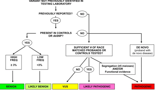
We relied on LMM’s standard variant assessment pipeline to create our dataset of manually classified variants. To ensure unbiased training and testing of our computational method, we excluded from manual classification information that was accessible to the method such as evolutionary conserva-tion or structural data, even though this informaconserva-tion is currently used in the pipeline. Each variant recieved a classification of “Pathogenic,” “Likely Pathogenic,” “Benign,” “Likely Benign,” or “Un-known Significance” (VUS). The basic decision process we used is described below and shown in Figure 1.1.

Pathogenic.Variants with a minimum of five informative meioses supporting familial co-segregation with HCM, absent in healthy controls, and/or having strong functional data are classified as pathogenic. In HCM, informative meioses typically only include individuals who are positive for both phenotype and genotype. This level of stringency is required due to the highly vari-able expressivity and reduced penetrance, which makes individuals without the phenotype largely uninformative, regardless of their genotype.

Likely Pathogenic.The minimum requirement to classify a variant as likely pathogenic is absence from race-matched controls or a large cohort of race-matched probands. The LMM has pre-viously sequenced sarcomere genes in over 1000 HCM probands of European ancestry. Ab-sence from this cohort was accepted in lieu of healthy control data because it serves to set

(25)

VARIANT NOT PREVIOUSLY IDENTIFIED IN TESTING LABORATORY

YES

HIGH

FREQ FREQLOW

! 3%

BENIGN

<3%

LIKELY BENIGN VUS

SUFFICIENT # OF RACE MATCHED PROBANDS OR

CONTROLS TESTED?

LIKELY PATHOGENIC PATHOGENIC NO NO YES YES NO DE NOVO (proband with de novo disease) Segregation (!5 meioses) AND/OR Functional evidence PRESENT IN CONTROLS OR dbSNP? PREVIOUSLY REPORTED? Sunday, June 20, 2010

Figure 1.1:Process used to classify variants at the LMM. This process is described in detail in 1.2. We treat the “Pathogenic”, “Benign”, and “Likely Benign” categories as high-confidence classifications for the purposes of training the automatic classifier.

(26)

variants detected in minority populations are therefore often classified as of “Unknown Sig-nificance” due to the lack of control cohorts or large proband data sets.

BenignorLikely Benign.Variants that are frequent in the general population (at least 3%) are clas-sified as “Benign.” Variants present in controls at frequencies below 3% and without other suspicion for pathogenicity are classified as “Likely Benign.”

Unknown Signiﬁcance (VUS).This class commonly includes variants for which there is insufficient evidence to classify the variant in any of the other four categories, or variants for which the evidence is conflicting.

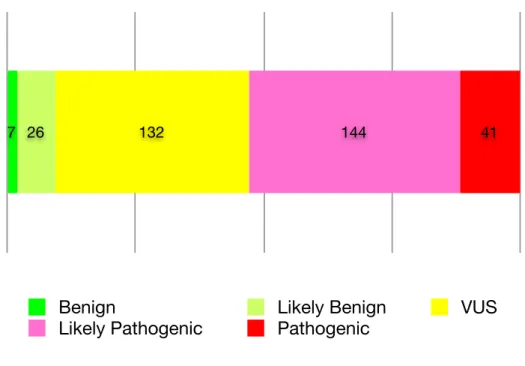
Figure 1.2 shows the distribution of variants by the classification category in our database.

After applying these criteria to the complete set of variants collected by LMM, we filtered the re-sulting dataset to exclude unconfident predictions. We excluded variants in the “Likely Pathogenic” category, considering the classification for this category not to be stringent enough. We also ex-cluded variants in the “Unknown Significance” category, since this category carries no clinical or bio-logical significance. This left us with 41 “Pathogenic” variants, which we treated as truly pathogenic, and 7 “Benign” and 26 “Likely Benign” variants, all of which we treated as truly benign. These 74 variants became our gold standard for validation of our predictor. The complete list of 74 variants is shown in Supplemental Table S1.

There is a possibility that the manual method of variant classification may have selected variants resulting in the most severe phenotypes, such as those seen in early onset cases, which may reduce the utility of our classifier for less severe variants. To investigate this possibility, we used the age at which an individual was tested as a proxy for age at onset. The distribution of ages of all probands tested is roughly trimodal with clear peaks at less than 1 and 15 years of age and a broad distribution centered around 50 years of age (Supplemental Figure S1). The distribution of pathogenic variants in

(27)

Benign Likely Benign VUS Likely Pathogenic Pathogenic 7 26 132 144 41

41

144

132

26

7 Benign

Likely Benign

VUS

Likely Pathogenic

Pathogenic

41 144

132 26

7

Benign

Likely Benign

VUS

Likely Pathogenic

Pathogenic

Figure 1.2:Distribution of variant pathogenicity. We categorized 350 missense variants in six genes according to the criteria described in Figure 1.1. The three categories “Pathogenic,” “Benign,” and “Likely Benign” were treated as high-confidence classifications and used as training data for our classifier (enumerated in Supplemental Table S1).

(28)

of age groups tested. If we were indeed selecting for only the most severe, early onset phenotypes, we would expect pathogenic variants to be over-represented in newborns and teenagers and to be absent in late-onset cases. This does not appear to be the case and we are confident that our training set does not only consist of pathogenic variants that lead to high penetrance, early onset disease.

1.2.3 Predictive features

We used four features in the final predictor. These features are described below.

PolyPhen-2 prediction.Our first feature was a prediction made by the existing method PolyPhen-22. PolyPhen-2’s predictions integrate several sources of phylogenetic and structural informa-tion using a Naive Bayes classifier. Its output represents a general-purpose predicinforma-tion, made without knowledge of the specific disease under consideration. The PolyPhen-2 software re-ports a score ranging from 0 (neutral) to 1 (damaging), which represents the confidence of its internal classifier. We used this integrated score as a single feature in our predictor.

MrBayes substitution rate score.Our second feature was the rate of evolution for each site in each gene. We computed this using the Markov Chain Monte Carlo (MCMC) algorithm in the MrBayes software package161. This score took several days of computer time to calculate for all six genes, and would not have been feasible to calculate for a genome-wide dataset.

Examples of the MrBayes instruction files we used are available as Supplemental Figure S2. We used a function that infers site-specific evolution rates and includes them in the program’s output. MrBayes reports the rate at positions with insufficient alignment depth as 1.000, so all scores of exactly 1.000 were treated as missing data. We normalized this rate so that the mean rate for each gene was 1.000.

(29)

andTPM1. We used the COILS2 software to predict the tendencies of the wild-type and mutant sequences to form coiled coils125,126. Variants that significantly change the coiled-coil tendency of the sequence are likely to interfere with protein function.

For each of the four proteins, we downloaded annotations from SMART to determine the locations of coiled-coil regions120. For any variant in a coiled-coil region, we ran COILS2 on both the wild-type and variant sequences of the coiled-coil region that contained the vari-ant. COILS2 outputs a score indicating coiled-coil tendency for each residue in the input sequence, with each score depending on the entire sequence. The feature we used in the final predictor was the magnitude of the largest single-residue change.

Protein structure comparison score.Four of the six target proteins are contractile proteins studied in multiple conformations (MYH7andMYL2in ATP, ADP and nucleotide-free states;

TNNI3andTNNT2in Ca2+activated and Ca2+free states). For these four proteins, we mea-sured the motion of each residue between the two conformations. Highly mobile residues were considered functionally important to the conformational change, while highly immo-bile residues were considered structurally important. Intermediately moimmo-bile residues were scored as unimportant. We measured the size of each residue’s motion by comparing the dis-placement of the residue to the expected probability distribution of disdis-placements under random thermal motion.

We used two sets of structures to compute this score. One was a set of six structures of a three-chain scallop myosin complex, consisting of the myosin heavy chain (corresponding toMYH7in human heart muscle) and the two myosin light chains (corresponding toMYL2

andMYL3in human heart muscle)82,87. One of these structures was not bound to a nu-cleotide (PDB ID 1KK7), two were bound to ADP analogs (PDB ID 1KK8 and 1B7T), and three were bound to ATP analogs (PDB ID 1KQM, 1KWO, and 1L2O). The other set of

(30)

structures was a pair of structures of a three-chain chicken troponin complex, consisting of troponin I (corresponding toTNNI3in human heart muscle), troponin T (corresponding toTNNT2in human heart muscle), and troponin C (corresponding toTNNC1in human heart muscle)188. One of these structures was activated by calcium ions (PDB ID 1YTZ), and the other had no calcium bound to it (PDB ID 1YV0).

We performed pairwise comparisons between structures that represented the same molecule in different biological states. Pairs of structures that represented the same biological state (such as 1KK8 and 1B7T, which both represent the ADP-bound state of myosin) were ex-cluded, under the assumption that differences between these structures would represent differences in the experimental preparation rather than a meaningful conformational change. We aligned each pair of structures with LovoAlign and measured the displacement between the alpha-carbons of corresponding residues129.

The variance in the position of an atom in a crystal structure is given by

σ2= B

8π2 (1.1)

whereBis the crystallographic temperature factor for the atom. We computed this variance for the alpha carbon of each residue, estimatingBas the average of the reported temperature factor for that atom across the two crystal structures. We used Student’s t-test to compare the squared displacement of the atom with its expected variance. This produced a p-value for the observed squared displacement, with numbers close to 0 representing motion much smaller than expected, numbers close to 1 representing motion much larger than expected, and numbers close to 0.5 representing the expected amount of motion. Finally, scores be-low 0.5 were subtracted from 1, so that a higher score would consistently represent a more

(31)

The human genes were aligned to the structures using BLAST. Each residue in the human sequence was scored the same as the residue it aligned to. Residues that did not align to the structures were not given a score. Only 84 human residues failed to align to the structures, which represents 3.2% of all positions in the four proteins to which we applied this score.

1.2.4 Multiple sequence alignments

Both PolyPhen-2 and the MrBayes score described above use comparative sequence analysis as a source of phylogenetic information. These methods take as input aligned sequences of multiple homologous proteins, and their predictive values critically depend on the quality of the multiple sequence alignments used. Existing computational methods, including PolyPhen-2 and SIFT, rely on automated pipelines to construct multiple sequence alignments2,142,143. We used the standard automated alignment pipeline provided by PolyPhen-2, but since we only needed to construct six alignments, we were able to inspect and adjust each alignment manually.

We noticed in our manual inspection that some of the automated alignments were of very poor quality. The worst alignments were for the two proteins that were most highly represented in our data set,MYBPC3andMYH7. These proteins have numerous homologs at the domain level, aris-ing from the multiple immunoglobulin domains ofMYBPC3and the highly conserved myosin motor domain ofMYH7, and the multiple sequence alignments produced using automatically se-lected homologs are therefore of poor quality. We created new alignments forMYBPC3andMYH7

by manually removing problematic sequences from the automatically generated alignments. This approach allowed us to tune the alignments manually while still taking advantage of PolyPhen-2’s automatic filtering of poor alignments and incorrect sequences. The alignments were very deep to begin with, allowing us to remove a large number of sequences without the alignments becoming too shallow to use.

(32)

domain-level homology to the target sequences and/or did not appear to have a sufficiently similar function to the target sequences. In other words, we attempted to create an alignment forMYBPC3that consisted only of forms of myosin binding protein C from various tissues and organisms, and an alignment forMYH7that consisted only of forms of myosin heavy chain from various tissues and organisms. The resulting alignments were used as input to the PolyPhen-2 classifier and to MrBayes. The sequences used are listed in Supplemental Tables S3–S6, and the resulting alignments are shown in Supplemental Figure S3.

1.2.5 Training and validation

We trained the classifier on the manually-curated set of 74 missense variants in 6 genes. For each variant in the training set, we computed the four features described above (PolyPhen-2 prediction, MrBayes substitution rate score, coiled-coil score, and protein structure comparison score). The val-ues of each feature for each variant can be found in Supplemental Table S2. The training algorithm (Supplemental Figure S4) aims to maximize accuracy of classification while keeping the required level of coverage. To avoid overfitting, the training algorithm uses ten-fold cross-validation (Supple-mental Figure S5). This method splits the training data into 10 parts (6 parts of 7 samples, 4 parts of 8 samples), trains the classifier on 9 training parts and tests it on the remaining 1 testing part. It then repeats the split-train-test procedure 10 times, each time with a different part of the data used for testing. In order to account for the different results that would be produced by using different ran-dom divisions of the data in this process, we ran 1,000 iterations of ten-fold cross validation, using a different random division of the data each time. We also tested the final classifier using a leave-one-out cross-validation strategy. The classifier assigns a prediction of “Pathogenic,” “Benign,” or “No Call” to each variant. The “No Call” prediction is given to variants the classifier cannot predict confidently. This category is included so that we can improve the accuracy (fraction of variants

(33)

pre-as either “Pathogenic” or “Benign”)153.

1.2.6 Feature selection

To verify that each of these four features made an important contribution, we constructed four in-complete classifiers, each one missing one of the four features. We performed validation on each of these classifiers as described above, and performed a random permutation test to show that the com-plete classifier had higher accuracy than each of the incomcom-plete classifiers. We performed 106 per-mutations, so that the minimum P-value we could find was 10−6. Out of our four features, only the PolyPhen-2 score had a one-sided P-value greater than this minimum, withp = 0.0544; the other three features all had one-sided P-values less than 10−6. We also performed the same test to establish that using manual alignments instead of automatic alignments improved the score, and found that it did with one-sided P-value less than 10−6. Figure 1.3 shows the distributions of accuracies for each set of features in 1,000 runs of cross validation.

In addition to the four features in our final classifier, we also tried replacing PolyPhen-2 with the similar tools SIFT and PANTHER142,143,180,181. We found that each performed comparably to PolyPhen-2, though the classifier with PolyPhen-2 performed very slightly better than either, again with one-sided P-values less than 10−6. Interestingly, though PolyPhen-2, SIFT, and PANTHER were each far more informative individually than any other single feature, each made by far the least individual contribution to the full four-feature classifier that included it. Evidently, the other three features together contain enough information to make the PolyPhen-2, SIFT, or PANTHER score largely redundant.

We also investigated the effect each feature had on coverage. This was of particular concern for the structure pair score and the coiled-coil score, each of which is missing entirely from several genes and regions, which could reduce the predictor’s ability to make confident classifications in these re-gions. We found that both the structure pair score and the coiled-coil score actually increase the

(34)

cov-Figure 1.3:Feature selection experiment. Each column shows the distribution of accuracies in 1,000 runs of cross-validation for a classifier built with a different set of features: “all features” represents the final four-feature classifier with manual alignments, “broken alignments” represents the four-feature without automatic alignments, and each of the other four columns represents a three-feature classifier missing the specified feature. Box plots show lower and upper quartiles (50% confidence intervals), and whiskers show 1.5 IQR ranges. The addition of each feature appears to improve the classifier, which is confirmed by a Mann-Whitney test.

(35)

erage, while neither of the other features has a significant effect. This suggests that it is rare for a vari-ant that could be scored confidently with the PolyPhen and substitution rate scores to be demoted to “No Call” because it is missing one or both of the other features. In other words, the coiled coil and structure pair scores tend to increase confidence where they are present rather than decreasing it where they are absent.

1.3 Results

1.3.1 The prediction method

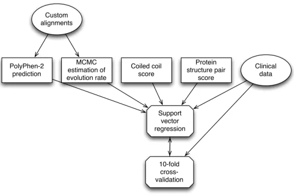
We created an automated method to predict the pathogenicity of missense variants in six genes known to contain variants that cause HCM. In designing this predictor, we set out to take advantage of the fact that we were focusing on a small set of functionally related genes to improve our predic-tions. We identified two ways to accomplish this: first, by exploiting unique structural and biochem-ical properties of the six target genes, and second, by applying more rigorous methods that would be difficult to implement for large numbers of genes. With these principles in mind, we developed a total of three predictive features, which we used in conjunction with the existing PolyPhen-2 clas-sifier2. Two of these features reflect specific structural properties of sarcomeric proteins. One scores the effect of amino acid change on coiled-coil regions, while the other scores the importance of the mutated residue to functionally important conformational transitions in ATP and Ca2+binding do-mains. The remaining feature is an estimated rate of evolution at the variant position. This feature was extremely time-consuming to compute and would not have been feasible to apply to a genome-wide dataset. It also was computed from manually adjusted multiple sequence alignments of homol-ogous sequences, which required human intervention to produce. These same manually adjusted alignments were also used as input to PolyPhen-2, improving its performance. We combined these three features and the PolyPhen-2 score using support vector regression, with our set of 74 manually

(36)

Custom alignments Coiled coil score Protein structure pair score PolyPhen-2 prediction MCMC estimation of evolution rate Support vector regression 10-fold cross-validation Clinical data

Figure 1.4:The automated prediction process. For each variant, we computed four features and combined them using support vector regression. We trained this classifier on the high-confidence variants classified with clinical data, and validated the classifier against the same data using ten-fold cross-validation.)

classified variants as a training set. The complete method is presented graphically in Figure 1.4. We also experimented with a small number of alternative features. The most notable among these were a different estimate of the rate of evolution computed using a genomic alignment of 46 vertebrate species, and several of the individual phylogenetic scores used as predictive features in PolyPhen-2. Addition of these features did not improve the performance of the predictor.

1.3.2 Validation of the method against manually classified variants Given the small size of our gold standard dataset (74 variants), the choice of training and valida-tion method was important. Because we had so few variants, it was not feasible for us to use the

(37)

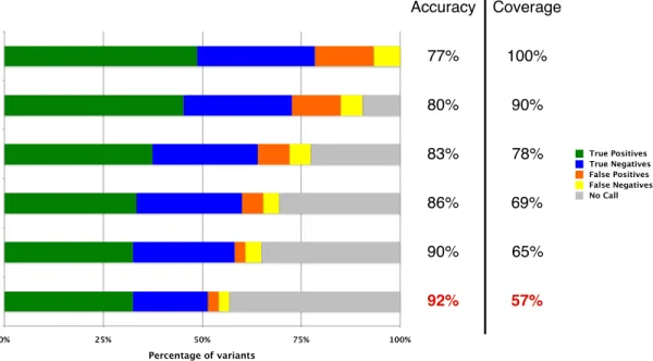
simplest validation method of splitting the dataset in half and using one half for training and the other for testing. Instead, we applied ten-fold cross validation, which is the accepted procedure in such cases (see 1.2.5). We ran this validation process a total of 1,000 times to obtain median results and confidence intervals. Figure 1.5 shows the results of this validation for six different classifiers at different levels of coverage and accuracy. We used the bottom row, highlighted in red, as our fi-nal classifier. The method predicts each variant as “Pathogenic,” “Benign,” or “No Call,” with the “No Call” result meaning that the predictor is not sufficiently confident to report a prediction. The median accuracy for covered variants for the most accurate classifier (the fraction of correct predic-tions out of all “Pathogenic” and “Benign” predicpredic-tions, while disregarding “No Call” results) was 92%, with a 95% confidence interval of 83%–98%. The median coverage (the fraction of variants that were predicted as either “Pathogenic” or “Benign”), was 57%, with a 95% confidence interval of 49%–64%; in other words, the median classifier reported “No Call” for 43% of variants. The median sensitivity for covered variants (the fraction of variants manually classified as pathogenic that were predicted as “Pathogenic,” excluding those predicted as “No Call”) was 94%, with a 95% confidence interval of 83%–98%. The median specificity for covered variants (estimated as the fraction of vari-ants manually classified as benign that were predicted as “Benign,” excluding those predicted as “No Call”) was 89%, with a 95% confidence interval of 83%–98%. The median odds ratio for a predic-tion of “Pathogenic” (the odds of a pathogenic variant being classified as “Pathogenic” divided by the odds of a benign variant being classified as “Pathogenic”) was 10, with a 95% confidence interval of 4.0–infinity (no upper bound could be set since more than 5% of trials had no false positives). The median odds ratio for a prediction of “Benign” (the odds of a benign variant being classified as “Benign” divided by the odds of a pathogenic variant being classified as benign) was 9.9, with a 95% confidence interval of 4.6–21. Leave-one-out cross validation also resulted in highly similar estimates of all these quantities.

(38)

Accuracy Coverage 77% 80% 83% 86% 90% 92% 100% 90% 78% 69% 65% 57% 0% 25% 50% 75% 100% Percentage of variants True Positives True Negatives False Positives False Negatives No Call

Figure 1.5:Results of cross validation. Rows contain median ten-fold cross validation results for the gold standard dataset at different levels of coverage. Horizontal bars correspond to different levels of coverage and median valida-tion coverage and accuracy levels are indicated. ‘True Positives’ are variants manually classified as “Pathogenic” that our method predicted as “Pathogenic.” ‘True Negatives’ are variants manually classified as “Benign” or “Likely Benign” that our method predicted as “Benign.” ‘False Positives’ are variants manually classified as “Benign” or “Likely Benign” that our method predicted as “Pathogenic.” ‘False Negatives’ are variants that manually classified as “Pathogenic” that our method predicted as “Benign.” ‘Uncovered’ are variants without a prediction (“No Call”). The bottom-most coverage level, indicated in red, was used for our final predictor.

(39)

1.3.3 Comparison with general-purpose methods

Since our predictor bases its predictions in part on predictions of the existing general-purpose method 2, we investigated whether our predictor was a significant improvement over the PolyPhen-2 predictor without our modifications and other general-purpose methods. In order to investigate this, we tested PolyPhen-2, SIFT, and PANTHER on the same dataset. We applied the same ten-fold cross-validation method with each of these three scores as the only predictive feature. We found that all three general-purpose scores had comparable performance on this dataset: PolyPhen-2’s me-dian cross-validation accuracy was 70% (95% confidence interval 60%–77%), SIFT’s was 74% (95% confidence interval 64%–83%), and PANTHER’s was 68% (95% confidence interval 56%–79%). All of these estimates are much lower than the accuracies reported for these methods, which may reflect features of this dataset. Our specialized predictor, on the other hand, had a median accuracy of 92% (95% confidence interval 83%–98%), as reported above. A permutation test showed that all three general-purpose predictors performed worse than our specialized predictor, with one-sided P-values of less than 10−6.

1.3.4 Predictions for variants without confident classifications

The ultimate goal of our predictor is to provide accurate predictions for variants that are not confi-dently classified by manual methods. This will not be possible if there is some systematic biological difference between the confident and unconfident classifications, such as a difference in penetrance, severity, or mechanism of disease. To determine whether this is the case, we applied our method to a low-confidence dataset, the set of missense variants that did not meet the confidence criteria to be manually classified as truly pathogenic or benign (Figure 1.6). Of the missense variants manually classified as “Likely Pathogenic,” 80% of those for which a prediction was made were predicted as “Pathogenic.” This is consistent with the expectation that most of these “Likely Pathogenic”

(40)

vari-0 30 60 90 120 150

VUS Likely Pathogenic

Predicted Benign Predicted Pathogenic No Call 56 57 25 58 70 18

Figure 1.6:Results for low-confidence dataset. Columns indicate, for each class of variants, the number of predictions in predicted categories produced by the final classifier.)

ants are indeed pathogenic. It is also consistent with the expectation that the fraction of variants predicted as “Pathogenic” in this set is lower than for variants manually classified as confidently pathogenic. Among variants manually classified as “Unknown Significance,” 70% of those for which a prediction was made were predicted as “Pathogenic.” Since these variants have been iden-tified in individuals diagnosed with HCM, there is a highera priorilikelihood that they are indeed pathogenic, although we have no way of knowing what the true fraction should be. The fraction of variants predicted as pathogenic remains lower in the “Unknown Significance” set than in the “Likely Pathogenic” set, which is consistent with what would be expected.

(41)

is well within the confidence interval of 49%–64% for the estimated coverage on the gold standard variants.

Discussion

We developed and clinically validated an automated method to predict the pathogenic effect of missense variants that might cause HCM. Unlike current commonly used methods, our predictor has been validated against high-confidence manually curated data. This enabled us to estimate its specificity and sensitivity for the specific task of predicting HCM mutations, which will allow its predictions to be incorporated into clinical reports to health care professionals as one piece of evi-dence supporting a variant classification. Although this tool adds little for variants whose clinical significance is already supported by strong genetic and/or functional data, it will add value for those variants that had little or no prospect of ever being supported by solid family studies or large scale healthy control studies. Importantly, our classifier is particularly helpful for variants identified in minority populations, where healthy control cohorts, one of the pillars of traditional variant classifi-cation, are typically unavailable.

To maintain high accuracy, it was necessary to sacrifice coverage, i.e. the proportion of variants for which a prediction is made153. As shown in Figure 1.5, an increase in coverage is accompanied by a rapid decline in accuracy. A method attempting to predict every variant as either pathogenic or benign could not achieve levels of accuracy acceptable for clinical use. We estimated the coverage of our predictor at 57%, with a 95% confidence interval of 49%–64%. We believe this level of coverage is still above the threshold of clinical usefulness. For comparison, note that out of 350 LMM missense variants in the six target genes, only 74 met the criteria for high-confidence manual classification, giving the manual classification process a coverage of only 21%. Note also that our method covers a different set of variants than the manual classification process, including 59% of the variants that the

(42)

manual classification classifies as “Unknown Significance.”

The most important limitation of our automated prediction method stems from the size of the training data set. In general, training on small data sets may lead to overfitting of automated clas-sifiers. An overfit classifier may be highly accurate on the training data but much less accurate on new data. We applied several safeguards against overfitting during training and validation. These in-cluded limiting the number of features in the classifier, using only features that we expecteda priori

to be informative, and performing cross-validation to calibrate parameters and estimate accuracy. In this way we hope we have avoided excessive overfitting in our final predictor.

It is important to point out that this method may not accurately predict the effect of those mis-sense variants that exert their effect partially or fully though affecting mRNA splicing. This is true for all currently available tools of this kind, including PolyPhen-2, SIFT, and others. For example, the MYBPC3 Glu258Lys variant was confidently manually classified as “Pathogenic” but was incor-rectly classified as “Benign” in several runs of cross validation (though not in the final predictor). Many MYBPC3 variants affect splicing and there is evidence that the Glu258Lys variant is disease-causing via this mechanism. The underlying cDNA alteration is c.772G>A, which affects the last base of exon 6. This position is known to be part of the splice consensus and 5 different splice pre-dictors (SpliceSiteFinder-like, MatEntScan, NNSPLICE, GeneSplicer and Human Splice Finder; see Supplemental Figure S6) predict an impact on splicing. This is supported by evidence showing that this may result in skipping of exon six5,128. Therefore, the conservation of the nucleotide and not the amino acid at this position is essential, possibly explaining a misprediction by our predictor. This is a limitation of this method and clearly lends itself to future improvement and generation of tools that incorporate a splice assessment.

It is also important to point out that clinical laboratories are typically aware of this limitation. Novel variant assessment is a lengthy and complex process that relies on a large collection of