By
Naiem Khodabandehloo Yeganeh
in fulfilment of the Degree of Doctorate of Philosophy School of Information Technology and Electrical Engineering
April 2012
I would like to thank these people, but . . .
• insert author list insert paper title. (submitted to insert journal name)
• insert author list insert paper title. insert journal name insert volume number, insert article or page number (insert year)
The issue of data quality is gaining importance as individuals as well as corporations are increasingly relying on multiple, often external sources of data to make decisions. Traditional query systems do not factor in data quality considerations in their response. Studies into the diverse interpretations of data quality indicate that fitness for use is a fundamental criteria in the evaluation of data quality. In this report we address the issue of quality aware query systems by developing a query answering methodology that considers user data quality preferences over a proposed collaborative systems architecture. In this report we present three major issues relating to quality aware queries, namely modelling of user data quality preferences, measuring source quality and processing the query considering those preferences and measures. We then address each of these issues by introducing Quality Aware SQL, Quality Aware Metadata and Quality Aware Source Ranking methods respectively. Proposed contributions are evaluated using a .Net tool called Quality Aware Query Studio which is developed to support our contributions and simulate the proposed multi source
architecture. Finally roadmap and timeline of future works is presented based on open challenges and remaining issues for the three mentioned challenges.
Acknowledgements iii
List of Publications v
Abstract vii
List of Figures xiii
List of Tables xv
1 Introduction 1
2 Framework for DQ Aware Query Systems 7
3 Related Work 13
3.0.1 Data Quality Framework . . . 15 3.0.2 Profiling Data Quality . . . 16
3.0.3 User Preferences on Data Quality . . . 17
3.0.4 Query Planning and Data Integration . . . 18
4 Conditional Data Quality Profiling 21 4.1 DQ Profile Table Approach . . . 24
4.1.1 Conditional DQ Profile Generation . . . 25
4.1.2 Complexity of the Proposed Algorithms . . . 31
4.1.3 Querying Conditional DQ Profile to Estimate Query Result . . . 32
4.1.4 Evaluation . . . 33
4.2 DQ Sample Trie Approach . . . 38
4.2.1 Sample Trie . . . 41
4.2.2 Sample Trie Algorithm . . . 45
4.2.3 Evaluation and Analysis . . . 56
4.3 Summary . . . 61
5 Quality Aware SQL 63 5.1 Inconsistent Partial Order Graphs . . . 66
5.2 Inconsistency Detection . . . 68
5.3 Normalization of DQ Preferences for Query Planners . . . 71
5.4 Summary . . . 73
6 Quality Aware Query Response 75 6.1 Estimation of the DQ of a query plan . . . 79
6.1.2 Sampling Based Approach . . . 82
6.1.3 Extension of Conditional DQ Profiling . . . 83
6.2 Summary . . . 83
7 Proof of Concept 85 7.1 Implementation of DQAQS . . . 86
7.1.1 Common Protocol Between Components . . . 87
7.1.2 Registering Data Sources . . . 90
7.1.3 Data Profiler . . . 90 7.1.4 Query Parser . . . 97 7.1.5 Query Planner . . . 99 7.1.6 Final Results . . . 100 7.2 Summary . . . 101 8 Conclusion 103 References 105
2.1 Data Quality Aware Query System Architecture . . . 8 2.2 A traditional data quality profile for a sample dataset . . . 10
4.1 A sample conditional DQ profile’s initial generation (a) the source data set (b) the expansion phase of conditional DQ profile . . . 27 4.2 Reduced conditional DQ profile of Figure 4.1 with thresholdsτ = 2 and= 0.2. 30 4.3 Comparison of the average estimation error rate for traditional DQ profile
(DQP) and conditional DQ profile (CDQP) for different variations in distri-bution of dirty data d. . . 35 4.4 (a) Effect of Error Distributiond on Profile Size (b) Effect of Error
Distribu-tion on profile generaDistribu-tion time . . . 36 4.5 (a) Effect of certainty threshold on the size of DQ profile for different
min-imum set thresholds τ (b) Effect of τ on estimation capability of the DQ profile . . . 37
4.6 Scalability graphs (a) generated profile size versus data set size (b) profile
generation time vs database size . . . 38
4.7 Sample trie and a query workload . . . 42
4.8 Normalizing popularity and cost for cost model calculation . . . 50
4.9 One dimensional illustration of the coverage of samples with different sampling rate d0 > d1 > d2 > d3 . . . 54
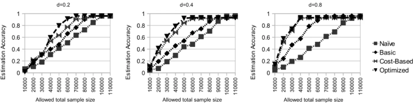
4.10 Effect of coverage don the effectiveness of approaches when query popularity is predictable . . . 59
4.11 Effect of coverage don the effectiveness of approaches when query popularity is constantly changing . . . 60
4.12 Effect of the uniform sampling rate selected on the effectiveness of approaches 60 5.1 (a)Circular inconsistency (b) Path inconsistency (c)Consistent graph . . . . 66
5.2 Graph G with a circular inconsistency and its relevant distance matrix . . . 69
7.1 Component architecture of DQAQS implementation . . . 87
7.2 Registering a new data source in DQAQS . . . 91
7.3 Generating an attribute based DQ profile in DQAQS . . . 92
7.4 Generating a conditional DQ profile in DQAQS . . . 94
7.5 Generating a sample trie based on a query workload in DQAQS . . . 95
7.6 Capturing user preferences using DQ aware SQL in DQAQS . . . 97
7.7 Capturing user preferences using visual tool in DQAQS . . . 98
7.8 Optimization of query plans ins DQAQS . . . 100
1
Introduction
User satisfaction from a query response is a complex problem encompassing various dimen-sions including both the efficiency as well as the quality of the response. Quality in turn includes several dimensions such as completeness, currency, accuracy, relevance an many more [33]. In order to present the best possible query response to the user, understanding user preferences on data quality as well as understanding the quality of data sources are
critical.
Consider for example a virtual store that is integrating a comparative price list for a given product (such as Google products) through a meta search (a search that queries results of other search engines and selects best possible results amongst them). The search engine obviously does not read all the millions of results for a search and does not return millions of records to the user. It normally selects top results from different search engines and compiles the answers from the shortlisted sources.
In the above scenario, when a user queries for a product, the virtual store searches through a variety of data sources for that item, ranks them and returns the results. For example the user may query for “Canon EOS”. In turn the virtual store may query camera vendor sites and return the results. The value that the user associates with the query result is clearly subjective and related to the user’s intended requirements which go beyond the entered query term, namely “Canon EOS” (currently returns 91,000 results from Google products). For example the user may be interested in comparing product prices, or the user may be interested in information on latest models.
More precisely, suppose that the various data sources can be accessed through a schema consisting of attributes (“Item Title”, “Item Description”, “Numbers Available”, “Price”, “Tax”, “User Comments”). A user searching for “Canon EOS” may actually be interested in:
1. Browsing products: such a user may not care about the “Numbers Available” and “Tax” columns. “Price” is somewhat important to the user although obsoleteness and inaccuracy in price values can be tolerated. However, consistency of “Item Title” and
completeness within the populations of “User Comments” in the query results, is of highest importance.
2. Comparing prices: where the user is sure about the item to purchase but is searching for the best price. Obviously “Price” and “Tax” fields have the greatest importance in this case. They should be current and accurate. ”Numbers Available” is also important although slight inaccuracies in this column are acceptable as any number more than 1 will be sufficient.
The above examples indicate that getting satisfactory query result is subjected to three questions: how good is each data source? what does the term “good” mean to the user? and how to assimilate data from the sources to best meet user preferences? To answer above questions, we face the following challenges.
First challenge is to provide suitable means to measure the quality of data. In order to estimate the quality of data we should collect descriptive and/or statistical information about data. These measures can in turn be used in query planning, and query optimization. Descriptiveness of the collected information contributes to the effectiveness of the system, by making predictions on the quality of the source/result-set closer to reality. However, it comes with a trade-off due to increased storage and computational costs. Although, in today’s technology, data storage is rarely a problem, and user satisfaction with the query results can be deemed more important than storage. In many real world applications, measuring DQ is not cheap. For example assurance of correctness of a url, is only possible by calling the url and parsing the returned page. Cost of such DQ measurements for millions of records, can be overwhelming. For such applications, efficient sampling techniques could be used for
profiling data quality. Generation of a minimal sample for estimating DQ profile in presence of environmental constraints is a key challenge.
Second challenge relates to the capture of user preferences on DQ. Modelling user pref-erences is a challenging problem due to its inherent subjective nature [28]. Additionally, DQ preferences have a hierarchical nature, since there can be a list of different DQ requirements for each attribute in the query. Several models have been developed to model user prefer-ences in decision making theory [28] and database research [20]. Models which have been based on partial orders are shown to be effective in many cases [29]. Different extensions to the standard SQL have also been proposed to define a preference language [20]. A good system for capturing user preferences should assist users to present consistent preferences as there is evidence to indicate that specification of user preferences on queries often contains irrational or inconsistent preferences [18].
Third challenge is to develop data quality aware query planning and data integration methods that allow for efficient data source selection and effective data integration in the presence of pre-specified user preferences. In particular, techniques for ranking data sources based on a multi-criteria decision making and assembling the results from the selected data sources into one query result are discussed in this paper.
In this paper we present a framework for DQ aware query systems in the presence of multiple overlapping data sources available for answering the same query. We define this framework around the three challenges mentioned earlier in this section which leads us to three key components of the system: 1) Profiling DQ which is the process of extracting mea-sures about the quality of each data source for a given query. 2) Capturing user preferences
on DQ and 3) Planning queries and integrating results from multiple sources in consideration of user defined DQ preferences.
The rest of this paper is organized as follows: In Section 2 the general framework proposed for this work is presented. Rest of the sections are dedicated to discuss solutions and options for the three challenges noted above. At the end of each section, relevant future works and open questions are discussed where relevant. Various techniques discussed in this paper are evaluated at the end of each section. In Section 3, existing literature related to the three key requirements of the framework is studied. Finally in Section 8 we conclude the paper.
2
Framework for DQ Aware Query Systems
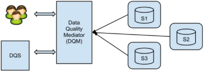
The challenges addressed in this research are positioned within an overall framework, namely Data Quality Aware Query System (DQAQS). Before starting the discussion about the framework for DQ aware query system, we assume the following architecture which is an extension of general data integration architecture with Data quality components. The ar-chitecture which consists of: Data sources (S1, S2, . . .), Data Quality Services (DQS), and
S1 S2 S3 Data Quality Mediator (DQM) DQS
Figure 2.1: Data Quality Aware Query System Architecture
a Data Quality Aware Mediator (DQM).
Data sources should expose their schema to the mediators. In general data integration systems this happens through a wrapper which is a component that wraps the database schema in order to unify the schemas definition for all sources. In this paper we assume the wrapper as part of the interface to the data source. The Data Quality Services are merely containers for DQ metrics and their definitions. They know about the business rules to measure DQ metrics and implement the functionality for it. Notion of the Data Quality Services is widely used in industrial products such as IBM Data Quality Stage, recent MS SQL Server Data Quality Services, etc. DQSs query relevant data sources to generate and maintain DQ profiles. Query mediators are the most complex part of the architecture and orchestrate query planning and data integration for the end user. Measurement of DQ is expensive, therefore, Data Quality services may become the bottleneck for processing data. They are usually able to process limited amount of data at each time and they are not able to process the data with the same speed that query response is generated by DQ Mediator. Therefore, DQ Mediator should use some terms of pre-processing if it wants to be able to provide DQ metrics to the user’s query.
DQ aware query languages, a service for planning the query and integrating data while considering DQ preferences and requirements, and a local DQ Profile Dictionary which potentially contains DQ profiles for all data sources. This profile dictionary can help the mediator to optimize its query plan and select only those data sources that best serve the user’s DQ preferences.
The effective and efficient deployment of the DQM as presented in the architecture above is a key objective of this paper. In the following sections we essentially present the techniques and methods necessary to build such a technology. Note that the three parts of the DQM correspond to the three challenges outlined in the introduction section, and represent the core elements of a data quality aware query system.
Measurement of the data quality of a data set is called DQ profiling. Overall statistical measurements for a data set - which we call traditional DQ profile - as shown in Figure 2.2 is used in literature and industry [34][24]. Figure 2.2 (b) represents a traditional DQ profile for the given data set of Figure 2.2 (a). DQ profile of Figure 2.2 (b) is the result of measuring completeness of each attribute in the dataset presented in Figure 2.2 (a). In this example completeness is considered as the number of null values over the number of records in the data for each attribute. For example, completeness of the “Image” attribute of the given data set is 50% since there are 3 null values over 6 records. The three columns in the profile table of Figure 2.2 (b) identify object (an attribute from the relation) against which the metric Completeness is measured as well as the result of this measurement.
Traditional DQ profiles which are similar to the one in Figure 2.2 (b) are incapable of returning reliable estimates for the quality of the result set most of the times. For example;
Figure 2.2: A traditional data quality profile for a sample dataset
even though the completeness of the Image attribute for data source S1 is 50%, the
com-pleteness of the Image attribute for query results (with conditions) from this data source can be anything between 0% and 100%: Completeness of the Image attribute for “Cannon” cameras is 50%, this value is 100% for “Sony” cameras, and 0% for “Panasonic” cameras. In reality, for example a Cannon shop may have records of other brands in their database, but they are particularly careful about their own items, which means the quality of Cannon items in database will significantly differ from the overall quality of the database. In this example, the selection conditions (brand is “Cannon” or brand is “Sony”) are fundamental parts of the query. However, they have not been considered in previous work on data quality profiling. In the next sections we propose the concept of conditional DQ profiling, along with techniques for generation and maintenance of the profile in two different environment. One techniques takes a closed-world assumption and guarantees the accuracy of DQ estimation which is more suitable for enterprise applications. We extend the discussion on creation and maintenance of conditional DQ profiles with proposing sampling techniques to estimate DQ for open world systems (e.g. Web), where environmental is more restrictive.
planning in data integration systems is selecting data sources. One method to rank data sources considering the quality of data sources and user preferences on DQ can be based on a multi-criteria decision making technique. The general idea of having a hierarchy in decision making and definition of hierarchy as strict partial orders is widely studied. In [28] a decision making approach is proposed which is called Analytical Hierarchy Process (AHP). Processing the problem of source selection for Quality-aware queries can be delineated as a decision making problem in which a source of information should be selected based on a hierarchy of user preferences that defines what a good source is.
3
Related Work
Consequences of poor quality of data have been experienced in almost all domains. From the research perspective, data quality has been addressed in different contexts, including statistics, management science, and computer science [30]. To understand the concept, various research works have defined a number of quality dimensions [30] [32].
Data quality dimensions characterize data properties e.g. accuracy, currency, complete-ness etc. Many dimensions are defined for assessment of quality of data that give us the means to measure the quality of data. Data Quality dimensions can be very subjective (e.g. ease of use, expandability, objectivity, etc.).
To address the problems that stem from the various data quality dimensions, the ap-proaches can be broadly classified into investigative, preventative and corrective. Inves-tigative approaches essentially provide the ability to assess the level of data quality and is generally provided through data profiling tools. Many sophisticated commercial profiling tools exist [13]. There are several interpretations of dimensions (which may vary for dif-ferent use cases), e.g. completeness may represent missing tuples (open world assumption) [3]. Accuracy may represent the distance from truth in the real world. Such interpretations are difficult if not impossible to measure through computational means and hence in the subsequent discussion, the interpretation of these dimensions is assumed as a set of DQ rules.
A variety of solutions have also been proposed for preventative and corrective aspects of data quality management. These solutions can be categorized into the following broad groups : Semantic integrity constraints [7]. Record linkage solutions. Record linkage has been addressed through approximate matching [16], de-duplicating [17] and entity resolu-tion techniques [4]. Data lineage or provenance soluresolu-tions are classified as annotaresolu-tion and non-annotation based approaches where back tracing is suggested to address auditory or reliability problems [31]. Data uncertainty and probabilistic databases are another impor-tant consideration in data quality [22]. In [19], the issue of data imputation for incomplete
datasets is studied, whereas maximizing data currency has been addressed in [27]
Nevertheless, data quality problems can not be completely corrected and in presence of errors and further consideration is required to maximise user satisfaction for the quality of data received.
3.0.1
Data Quality Framework
A number of studies have focused on answering queries in information systems based on some aspects of the data quality. Quality-aware querying performed by Data Quality broker is explicitly addressed in some works. In [23] a service based framework for representing and exchanging data quality in cooperative information systems is described. A data quality broker monitors the communication within the system and manages a number of DQ metrics (e.g. trustworthy, currency, etc.) of data sources. Similarly, DaQuinCIS architecture was proposed at [3] to manage DQ in cooperative information systems. Both these architectures define certain data quality metrics and suggest techniques to manage them for different data sources using a distributed service called Data Quality broker. In [24], a model for determining the completeness of a source or combination of sources is suggested. In [24] an algorithm for querying the most complete data is proposed which selects the sources with the highest completeness to answer a query. In addition of the above works, [8] analyzes existing definitions and metrics for data freshness in the context of a Data Integration System.
We share with above works, the idea of data quality aware querying; however the main difference is the semantics of our system: Our aim is not only to query quality of data sources or data, but is to improve the user satisfaction from the query results. To such a
scope, profiling data quality to estimate DQ with high accuracy for the final query result, should go to the extent of estimating DQ of any given query with various selection conditions. Additionally understanding user preferences on data quality is not studied in the above works ([23] proposes Xml based method to model DQ metrics assignments, but does not cover the problem of capturing user preferences on data quality). One more difference between the semantics of our system and above works is that we de-coupled our system with the definition of the DQ metrics, and focus on the problem of DQ profiling and query answering in isolation from the DQ definition.
3.0.2
Profiling Data Quality
Measurements made on a dataset for DQ dimensions are called DQ metrics and the act of generating DQ metrics for DQ dimensions is called DQ profiling. Profiling generally consists of collecting descriptive statistical information about data. These statistics can in turn be used in query planning, and query optimization. Data quality profile is a form of meta data which can be made available to the query planning engine to predict and optimize the quality of query results.
Literature reports on some works on DQ profiling. For example in [24] DQ metrics are assigned to each data source in the form of a vector of DQ metrics and their values (source level). In [32] a vector of DQ metrics and their values is attached to the table’s meta data to store additional DQ profiling; e.g. {(Completeness,0.80),(Accuracy,0.75),. . .} (relation level). In [34] an additional DQ profile table is attached to the relation’s meta data to store DQ metric measurements for the relation’s attributes (attribute level).
We assume that a set of DQ metrics M is standardized between data sources, however data sources may have different approaches (i.e. different rules) to calculate their DQ metrics (e.g. a UK based data source has a different set of rules from an Australian based data source for checking accuracy of address). Above profiling technique provide estimation of the quality of data for a data source, a table or a static set of data. Although these works estimate the quality of data, the difference between our work and above works lies in the fact that we are interested in estimating the data quality of the query results based on the query requested by the user which contains selection conditions.
3.0.3
User Preferences on Data Quality
The issue of user preferences in database queries dates back to 1987 [21]. Preference queries in deductive databases are studied in [15]. In [20] and [9] a logical framework for formulating preferences and its embedding into relational query languages are proposed. We leverage the idea presented in these works in modeling user preferences, however none of these works specifically address the issue of modeling DQ preferences.
Additionally, several models have been developed to model user preferences by decision making theory and database communities. Models which have been based on partial orders are shown to be effective in many cases [29]. Typically models based on partial order let users define inconsistent preferences.
Current studies on user preferences in database systems assume that existence of incon-sistency is natural (and hard to avoid) for user preferences and a preference model should be designed to function even when user preferences are inconsistent, hence; they deliberately
opt to ignore it. Nevertheless, all studies do not always agree with this assumption [18]. Human science and decision making studies show that people struggle with an internal con-sistency check and they will almost always avoid inconsistent preferences if those individuals are given enough information about their state in their decision (e.g. visually). In fact, existence of inconsistency in user preferences dims the information about user preferences captured by the query.
All above works address the problem of understanding and modeling user preferences in different domains, from computer science to psychology. In regards to modeling user preferences in DQ, we share similar goals with above works, however we put together ideas from the different fields to present a practical model for capturing reliable user preferences on data quality.
3.0.4
Query Planning and Data Integration
From a query planning perspective, a data source is abstracted by the source descriptions. These descriptions specify the properties of the sources that the system needs to know in order to use their data. In addition to source schema, the source descriptions might also include information on the source: response time, coverage, completeness, timeliness, accuracy, and reliability, etc.
When a user poses a data integration query, the system formulates that query into sub-queries over the schemas of the data sources whose combination will form the answer to the original query. For applications with a large number of sources, typically the number of sub-query plans is very large and plan evaluation is costly, so executing all sub-query plans
is expensive and often infeasible. In practice, however, only a subset of those sub-queries is actually selected for execution [11][25][26].
Each executed sub-query is also optimized to produce a physical query execution plan with minimum cost. This plan specifies exactly the execution order of operations and the specific algorithm used for every operation (e.g., algorithms for joins). Existing techniques tend to separate the query selection process into two separate phases using two alternative approaches: 1) select-then-optimize, and 2) optimize-then-select. In the first approach, a subset of sub-queries is selected based on coverage, then each selected sub-query is optimized separately [11][25], whereas in the second approach, each sub-query is optimized first, then a subset of optimized sub-queries is selected to maximize coverage while minimizing cost [26]. However, in both approaches, the selection of query plans is primarily based on data coverage and/or query planning costs without further considerations for DQ. To the contrast, in this paper, we describe our approach for query plan ranking based on DQ that allows for efficient data source selection in the presence of pre-specified user preferences over multi-dimensional DQ measures.
4
Conditional Data Quality Profiling
DQ profiling is the task of measuring DQ metrics for given data. In this paper we assume that services exist which can measure DQ metrics (i.e. DQS as described in Section 2). In particular, we do not need to know how Completeness or Consistency of data is defined, instead we assume a service that calculates DQ metrics for every row of the dataset.
Data quality profile that stores attribute level DQ statistics for the whole dataset will 21
require very little amount of storage for each data source, an attribute level DQ profile is shown in Figure 2.2 (b). The DQ profile in Figure 2.2 is generated from the data set of Figure 2.2 (a). It is the result of measuring completeness of each attribute in the dataset presented in Figure 2.2 (a). In this example completeness is considered as number of null values over the number of records in the data for each attribute. For example the completeness of the “Image” attribute of the given data set is 50% since there are 3 null values over 6 records. The three columns in the profile table of Figure 2.2 (b) identify object (an attribute from the relation) against which the metric Completeness is measured, and the result of this measurement.
Attribute level DQ profiling (we also call it traditional DQ profiling) is not adequate for all purposes. Above limitation of traditional DQ profiling motivates us to proposeConditional DQ Profile to estimate DQ profile metrics where distribution of dirty data in dataset is not evenly random and queries are bound with conditions.
In this section, we propose techniques and methods to present the conept of conditional DQ profiling for a variety of needs and environments. Measuring DQ metrics is expensive. It often involves querying some external master data or refernce. Data Quality Service is responsible to measure DQ metrics for a given set of data and it is limited in the amount of data it can process in a timely fation. For example a DQS might be able to provide accuracy measures for only a few hundred addresses a second while source data sets have tens to hundreds of million records. Obviously the amount of data and the available preprocessing time wil have a signifact effect on the usefulness of the proposed DQ profiling technique.
user where the estimate is not far from the actual DQ with any more than a limitted pre-known error rate. We call this; guaranteed DQ estimation. Depending to the environmental restrictions and amount of data that should be profiled, guaranteed DQ estimation may or may not be achievable. For example in a corporate environemnt where the number of records in data sets are limitted and DQ profile can be generated overnight, user can have the luxury of guaranteed DQ estimation. In contrast on web or cloud environment where pre-processing all data sets is extremely costly and processing can not happen overnight, an incremental collaborative technique that can create DQ profiles within enforced cost limits is required.
In this paper we first propose techniques to generate a DQ profile that can guarantee DQ estimation, and is suitable for the corporate environment. We call this profile, DQ Profile Table, and we present a technique to generate and compress the DQ profile table by pre-processing all data in data sets. This technique can guarantee the accuracy of DQ estimation in trade off with procesing and storage cost of the profile creation and DQ measurement.
Afterwards, we propose a technique based on sampling data which works in presence of cost constraints on DQ measurement and does not asume pre-processing of the data-sets. We call this technique sampling trie. In sampling trie technique, we try to optimize the accuracy of DQ estimation within cost limits, however, we can not guarantee DQ estimation.
The two proposed techniques for DQ profile generation and maintenance can cover vari-ous environments in which DQAQS is implemented and contribute to the generality of the proposed framework.
4.1
DQ Profile Table Approach
Given a data set S, let us assume direct access to all data inS is possible and generation of the DQ profile is an off-line process, i.e. resources and time for preprocessing the whole data set is available. In order to define Conditional DQ Profile, we first need to formally define DQ metric function.
Definition 1.1 Let{a1, . . . , am}be all attributes of the relation R,T be a set of tuples
representingR, and metric mbe a set of rules. We define metric functionmai(t),t∈T as
1, if the value of attribute ai from tuple t, does not violate any rule in m, and 0 otherwise DQ metric function mai is a set of rules, where each rule is a boolean function that
describes DQ dimension. For example, accuracy metric function for a given postcode can be defined by a set of rules containing a check that compares data against some master data.
Assuming conditions in a finite domain consist of single comparisons, combined together with ∧ operators, we define Conditional DQ profile as a table that maps conjunctive condi-tions of queries to DQ metric values1. For every metric functionm
ai, we create a Conditional
DQ profile table which is as a set of conditional DQ profile records, and defined as below:
Definition 1.2 Let mai be an arbitrary metric function for attribute ai, and T be set
of tuples for relation R. We define conditional DQ profileP r as a set of DQ profile records
tP r.
Definition 1.3 LetP rbe a conditional DQ profile table, consisting of profile recordtP r,
and Condition be the set of conjunctive equality conditions for a given query that results in a subset of dataset ζ ⊆ T. We define tP r as (Condition) → (#ζ, Qζ), where Condition
is a query’s conjunctive selection condition and ζ is a subset of T that satisfies Condition. #ζ =|ζ| and Qζ =|{t ∈ζ|mai(t) = 1}|
In relational databases, we store the profile table P r for metric mai (also referred as
P rmai) as a relation (a1, . . . , an, a#, aQ) consisting of profile row tuplestP r = (t1P r, . . . , tnP r,#tP r, QtPr)
wheretiP r ∈dom(ai)∪“ ” (don’t care value). #tP r is number of appearances of the tuple in
T considering “ ” which substitutes for anything, and QtP r is the number of tuples among
them that return 1 for mai.
If we are given all possible conjunctive equality conditions that can happen for a given dataset, we can create the conditional DQ profile P rai for any given metric function.
How-ever, the number of possible conjunctive equality conditions over a given dataset can be exhaustive and the Conditional DQ Profile that would be created from all possible queries can become much larger that the underlying dataset.
4.1.1
Conditional DQ Profile Generation
As described above, the complete search space for a conditional DQ profile may need to traverse all condition possibilities.
Brute-force Approach Conditional DQ profile generation incurs the following challenge:
Size of a complete conditional DQ profile which has all data required for estimating the quality of any query result, can be as big as the original dataset or even larger. Thus, storing and querying conditional DQ profile may be too expensive and inappropriate.
(a) (we also refer as B, M, P for simplicity). Values these attributes come from the follow-ing domains: dom(B) = {Sony, Cannon} (abbreviated as {S,C}), dom(M)={SLR, Norm} ({S,N}), and dom(P)={Low, High}({L,H}). Each domain has 2 members, by addition of don’t care value (“ ”), there can be 33 possible queries. {B=C or B=S or B= , M=S or M=N
or M= , P=H or P=L or P= }. Search space consists of all possible subsets of equality com-parisons joined with∧operator (e.g. {B=C∧M=S∧P=H}). Number of possible comparisons for any attributeais|dom(a)|and search space can be as large as|dom(a1)|×. . .×|dom(an)|
where n is the number of attributes in R.
The brute-force solution is to enumerate all possible conjunctive equality selection condi-tions over dataset R, compute the metric function for each conjunctive condition and store DQ of the results and the conjunctive selection condition in DQ profile P r. P r can then be queried to estimate the quality of the result set for any given query with any selection condition.
The brute-force browsing of all possible conjunctive conditions is inefficient for two rea-sons: First, there are many selection conditions for which no result in the dataset can be found. For example if data set Item does not include tuple {Cannon, SLR, Low} (or {C,S,L}), it is not required to be checked. Second, measurement of the quality of the query result for each combination of conditions requires execution of a query (first, the query result set should be found, and then the data quality of that result can be calculated). Obviously there is a cost associated with each query.
Efficient Conditional DQ Profiling
Figure 4.1: A sample conditional DQ profile’s initial generation (a) the source data set (b) the
expansion phase of conditional DQ profile
further reduction of its size. We call the first phase of the technique as expansion phase where the initial conditional DQ profile is created. We call the second phase as reduction phase in which we reduce the profile size while maintaining acceptable accuracy of DQ estimation. We further have a revert phase that will be used to overcome any loss on information incurred during the reduction phase. The level of acceptability of accuracy is ensured by letting user define two thresholds which will be discussed further in this chapter. Leta1. . . ak be the list of attributes to be used for query conditions over R, and mai be
the metric function m on attribute ai to be profiled.
In initial phase, we create conditional DQ profile P r using the following query:
select a1. . . ak,count(ai) as #, sum(mai) as Qfrom R group by a1. . . ak
union
select a1. . . ak−1,’-’ as ak, count(ai) as #, sum(mai) as Qfrom R group by a1. . . ak−1
. . .
select a1, ’-’ asa2, . . ., ’-’ as ak, count(ai) as#, sum(mai) as Q from R group by a1
union
order bya1, . . ., ak
Above query creates the conditional DQ profile similar to Figure 4.1 (b). We now explain the above concept in the context of our running example. In Figure 4.1 we use completeness for metric function defined as one simple rule: “if Image is Null then 0 else 1”. Note that the same principle can be applied to other DQ metrics that can be defined through a rule or set of rules. Figure 4.1 (a) shows sample data set Items(Brand, Model, Price, Image). All attributes and their values are abbreviated to the first letter in Figure 4.1. Figure 4.1 (b) illustrates the conditional DQ profile before applying the threshold for estimating the Completeness of attribute Image. Profile created after the expansion phase, is usually large, therefore; we take further steps to reduce the size of generated profile.
Approximating DQ to Reduce Size We reduce size of the profile in two ways. First
by estimating the value of query’s DQ metric instead of providing the exact value and second, by removing all the conditions that return few and statistically insignificant number of records. These reductions are controlled by two thresholds: First, minimum set threshold
τ which defines the minimum size of tuple set to be profiled. For example if there is only four Panasonic cameras in a shop, andτ = 10, DQ profile row with conditionBrand =P anasonic
will not be created. This threshold will reduce noise in DQ profile, e.g. if this threshold is ignored (τ = 1), any single tuple which has the metric function value of exactly 0 or 1 appears in the conditional DQ profile. Second, certainty threshold is the maximum acceptable uncertainty for the user. For example, if = 0.1, the DQ profile row with condition Brand=Cannon should return completeness between 40% and 60% for data set in Figure 2.2.
Algorithm 1, receives conditional DQ profile tableP r, and accuracy thresholdas input, and returns a reduced conditional DQ profile table. Algorithm 1 removes profile records which their metric function value is within range of from their parent profile record. For a given profile record P rt1, a parent profile record P rt2 is a record which for every attribute value in P rt1, the same value or “−
00 exists in P r
t2. For example (C, S, ,4,2) is parent of (C, S, H,2,2).
Data: Profile TableP r
create empty stackS push(S,fetchxfromP r)
whileeof(P r)do
FetchxfromP r
ifxis parent oftop(S)or vice versathen
Lets:=top(S)
if(s.Q/s.#)−≤(x.Q/x.#)≤(s.Q/s.#) +then
deletexfromP r
end else
whiletop(S)is not parent ofxor vice versado
pop(S)
end end end returnP r
Algorithm 1: Reducing the size of conditional DQ profile
Algorithm 1, removes profile records from dataset where quality of the profile record is in range of from the quality of the closest parent record that is not deleted. For example as in Figure 4.2, recordS, , for which the quality (57%) is in the range of = 0.2 (or 20%) from its parent , , (63%) is removed from dataset. Hence, the quality of a query with condition Brand = S will be estimated from its closest parent 63% which is not far from the actual quality of the result-set (around 57%). Figure 4.2 (a) depicts the DQ profile from Figure 4.1 (b) considering τ = 2 and Figure 4.2 (b) shows the reduced profile table of the Figure 4.2 (a) considering = 0.2.
Figure 4.2: Reduced conditional DQ profile of Figure 4.1 with thresholdsτ = 2 and = 0.2.
Furthermore, reducing the size of profile by removing profile records that reflect less than
τ records is straight forward an it can be done using the command delete from P r where
#≤τ.
Although, Algorithm 1 is able to reduce size of the profile, it has the side effect of losing some valuable data. For example if DQ profile record S, S, H is removed, the quality of the query with condition P rice = H can not be estimated. Using Figure 4.2 (a), quality of
, , H can be estimated from the quality of records C, S, H, C, N, H, S, S, H, and S, N, H
(i.e. (2 + 2 + 0 + 0)/(2 + 3 + 1 + 1) = 57%), but using Figure 4.2 (b), such value can not be estimated correctly. This problem appears because we have reduced a record by comparing it to only one of the possible parents. For exampleS, S, H is not only a child ofS, S, in the search space. It can also be a child of S, , H or , S, H which do not exist in the generated DQ profile.
After reducing the DQ profile with the threshold , we reduce the profile with minimum set threshold τ.
To resolve this problem, if we are removing some records (nodes in the search space) from the profile, we should revert all possible parents of the removed nodes if removal of the node effects the correctness for DQ estimation for its parent. For example, if we are removing
S, S, H, and the quality of it’s parent node , S, H is different, we should revert , S, H into the conditional DQ profile. We revert any useful deleted data as follows; we refer to this part of the algorithm as Revert phase:
Given profile tablePr (a1, ..., an,#, Q), and all eliminated tuples C=(c0, . . ., cn, #, Q),
and a prefix list consisting of A = (ai, . . . , ak), let A+ be the attributes of P r that do not
appear in A. First, run expansion and reduction phases for C sorted by order sequence aj
where aj start with sequence A and continues in a random order from A+. Revert results
to P r with the depth of the recursion attached to it and keep reduced records inC0. Then, if |C0| ≤ |C| or A+ is null or C is null, for each attribute a0 ∈ A+, recursively run revert phase with parameters A=A∪a0, C0 and P r.
For example deleted records from Figure 4.2 (a) will be sent to revert phase in parallel, sorted as (P, M, B),(M, P, B). First recursion for the attributes sorted asP, M, B, generates
HSS,66%,H, S, ,66%,H, , ,66%, etc. It will be reduced toH, , ,65%, etc. Revert phase recurses for another level (as long as size of the result of the function is reducing).
Thus, generation of the conditional DQ profile now happens in three steps: First, run expansion, second; reduction phases of the algorithms over data, and third; run the revert algorithm for each attribute in P r to update P r.
4.1.2
Complexity of the Proposed Algorithms
Initial expansion phase of the algorithm, consists ofngroup by queries, wherenis the number of attributes that may appear in conditions. Group by queries run in O(|R|) where |R| is size of the relation R. Push and pops to the stack, in the Algorithm 1, happen exclusively,
thus they do not introduce extra complexity dimension. Complexity of the expansion and reduction phases of the algorithm is O(|R|.n) in worst case. For the Revert phase of the algorithm we conduct various experiments to compare execution time versus dataset size.
In traditional DQ profiling, a full scan of the database is required to figure out the average DQ profile of the whole dataset per metric O(|R|.n). However, expansion phase of the algorithm usually generates a much larger DQ profile. Reduction and revert phases of the algorithm take more preparation time in favour of a smaller conditional DQ profile.
4.1.3
Querying Conditional DQ Profile to Estimate Query Result
Conditional DQ profile can estimate the quality of the result set limited to the two factorsτ
and . There might be cases where query conditions do not exist in the profile, this happens for three reasons: 1) If the query returns no data. We assume checking for this situation occurs before querying the profile to avoid unnecessary reference to datasets that are not relevant. 2) The profile record might have been removed due to threshold. In this case, we return estimation for next available parent of the query in profile. 3) The profile record might have been removed due to threshold τ. In this case we act similar to the previous case, but the result can be inaccurate.
In previous section we proposed techniques to create conditional DQ profile for a given data set. Estimating DQ of the query result from a conditional DoQ profile is possible by finding the first row in the conditional DQ profile that contains all conjunctive selection conditions in the query. In worst case, a full scan of DQ profile may be required. Hence speed of query answering from conditional DQ profile is proportional to the size of DQ profile.
Consider relation R from the source S, and conditional DQ profile P r for an arbitrary metric and attribute. P r consists of columns (a0, . . . ,ak,#, Q). To estimate the quality
of the result set for user query consisting of selection criteria Φa0=α0∧...∧aj=αj, same query
should be run against the DQ profileP r(instead ofR), but it should also consider the don’t care values “ ”. We can translate Φ to Φ0(a
1=α0∨a1=“ 00,...). If ai is not mentioned in the query conditions, it still appears in the translation as ai = “ ”. For example query SELECT * FROM D WHERE Brand=“Cannon” AND Model=“SLR” translates to SELECT TOP 1 #, Q FROMP rWHERE (Brand=“Cannon” OR Brand=“ ”) AND (Model=“SLR” OR Model = “ ”) AND (Price=“ ”) ORDER BY Brand, Model,Price. In regards to the ORDER BY operation, don’t care “ 00 value should appear after any other value in the domain, hence, general result will be selected only if a less general result does not exist.
4.1.4
Evaluation
Here we study effectiveness and scalability of our proposed techniques of this section. Effec-tiveness of conditional DQ profile is compared against the traditional DQ profile. Traditional DQ profile generates only one value for the whole data set regardless of the underlying data. Therefore, it imposes very low overhead on the system. When distribution of dirty data is totally uniform through the whole dataset, our conditional DQ profile also seems to be very small. However, the benefits of our technique becomes obvious when distribution of dirty data in the data set is not totally uniform. In this section we only compare effectiveness of our approaches with traditional DQ profiling. In regards to scalability of profile creation,
traditional DQ profile has a constant cost, which is not comparable to our techniques. How-ever, we study scalability of our techniques versus various affecting factors. We study our algorithms on the publicly available DBLP data set [10].
In this paper, we assumed that details of the calculation of DQ metric is transparent for our technique. Hence we write a deterministic function that pre-generates a metric result value for every record of the dataset. This function stores the pre-generated results per record in a lookup table and returns the same result for every record of the dataset each time.
The important characteristic of the data that affects size of the conditional DQ profile, is distribution of dirty data. On one end, distribution of dirty data can be totally uniform. Then conditional DQ profile will be reduced down to traditional DQ profile and would need only one row to satisfy DQ estimation requirements for all the queries. On the other end, if any given subset of the dataset has a different distribution of dirty data from another conditional DQ profile should have one row for each subset.
In order to simulate different distribution of dirty data in data set, we pre-generate metric functions as follows: Let d be the variation in distribution of dirty data. d = 0 is no variation in distribution of dirty data, i.e. uniform distribution of dirty data, and d = 1 is the maximum variation in distribution of dirty data. We approximately simulate d by grouping the dataset by all attributes that can be used in the conditions. Then we generate
count(Groups)/d, (or 1 ifd= 0) random numbers and map these numbers to groups with the same pattern. For example, there might be 100 different groups for {Brand, M odel, P rice}. If d = 0.5, two random numbers, e.g. 0.3 and 0.9, will be generated and mapped to the
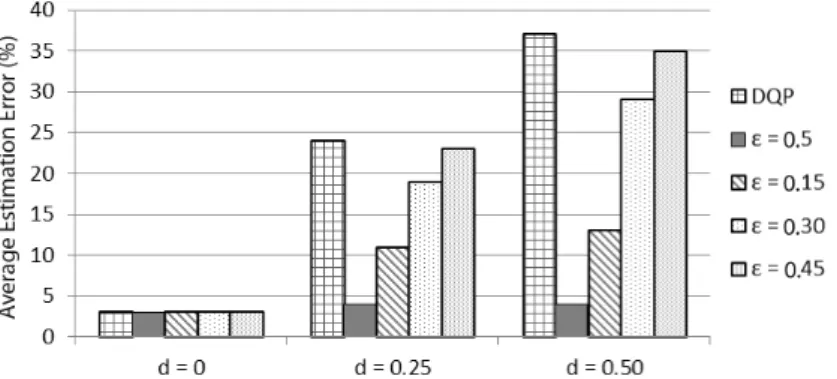
Figure 4.3: Comparison of the average estimation error rate for traditional DQ profile (DQP)
and conditional DQ profile (CDQP) for different variations in distribution of dirty data d
groups to introduce dirty data respectively. Therefore; division of dirty data for first 50 groups will be 0.3 and division of dirty data for the other 50 groups will be 0.9.
For evaluation of our techniques, we first generate the conditional DQ profile. To ensure we have covered different combinations, we run 10% of all possible queries with conjunctive equality selection conditions against the profile for each experiment. In order to better understand the effect of two different thresholds on DQ estimation quality, when measuring the effects of , we exclude all queries that return less than τ results.
Effectiveness of DQ Estimation Figure 4.3 shows the average error rates of randomly
generated queries. Figure 4.3 compares the average estimation error rate for both traditional DQ profiles (DQP) and conditional DQ profiles (CDQP) in case of different variations in distribution of dirty data. Estimation error rate is difference of the actual metric function value of the query result and estimated metric function value of the query result). Conditional DQ profile is generated for different thresholds = 0.15, = 0.30, and = 0.45. It can be observed that, estimation accuracy using conditional DQ profile has always better than . DQ estimation error rate in conditional DQ profile will not exceed the threshold .
d (Variation in distribution ofdirty data) d (Variation in distribution ofdirty data)
Figure 4.4: (a) Effect of Error Distribution d on Profile Size (b) Effect of Error Distribution
on profile generation time
performs as well as conditional DQ profile, however, when variation in distribution of dirty data increases, the actual metric function value for more queries will be different from the traditional DQ metric estimation which is basically average of DQ metric value for the whole dataset. Therefore, estimation error will increase. Higher also means that much more profile records are reduced and DQ metric value for more queries are not estimated correctly.
Effect of Error DistributionFigure 4.4 (a) and (b) show the effect of variation in distri-bution of dirty data on database size and the cost of creating conditional DQ profile. We conducted this experiment on a windows 7, 32 bit virtual machine with 4GB of RAM on a Intel Core i3 2GHz machine running OSX as the host operating system. It can be observed that uniform distribution of dirty data results in the minimum profile size. Indeed, if for example from every 10 records in the dataset, 7 are of good quality, any arbitrary subset of the dataset will return 70% for the metric function. Hence, it might be enough to only keep the metric function result for the whole data set. However, when the distribution of dirty data increases, a bigger profile will be required. Based on Figure 4.4 (b) although the
Figure 4.5: (a) Effect of certainty threshold on the size of DQ profile for different minimum
set thresholds τ (b) Effect ofτ on estimation capability of the DQ profile
profile size increases by more variation in distribution of dirty data, profile generation time decreases with increase in variation of the distribution of dirty data. The reason for this behaviour is that most of the profile generation time is spent in the reduction phase.
Effect of and τ ThresholdsFigure 4.5 studies the effect of both minimum set threshold
τ and accuracy threshold on size of the conditional DQ profile. It can be observed that with tolerating a degree of uncertainty, a significant reduction in the DQ profile size can be achieved. Thresholds τ and improve size reduction if they are used together, e.g. a very low τ and relatively high has a negative effect on the generated profile size. A higher
means lower accuracy. Figure 4.5 (b) depicts the effect of minimum set threshold τ on the estimation capability of the DQ profile. Since DQ is statistical characteristic of data, τ = 0 means that if a query results in only one or two records, DQ profile row for supporting that query should be kept in the profile table, however, in many applications only a few records, do not convey statistical significance. In contrary, increasing τ to a big number will remove many possibly valuable profile records from the profile table which DQ metric for them can not be estimated, and we may need to fall back to traditional DQ metric estimate for those queries.
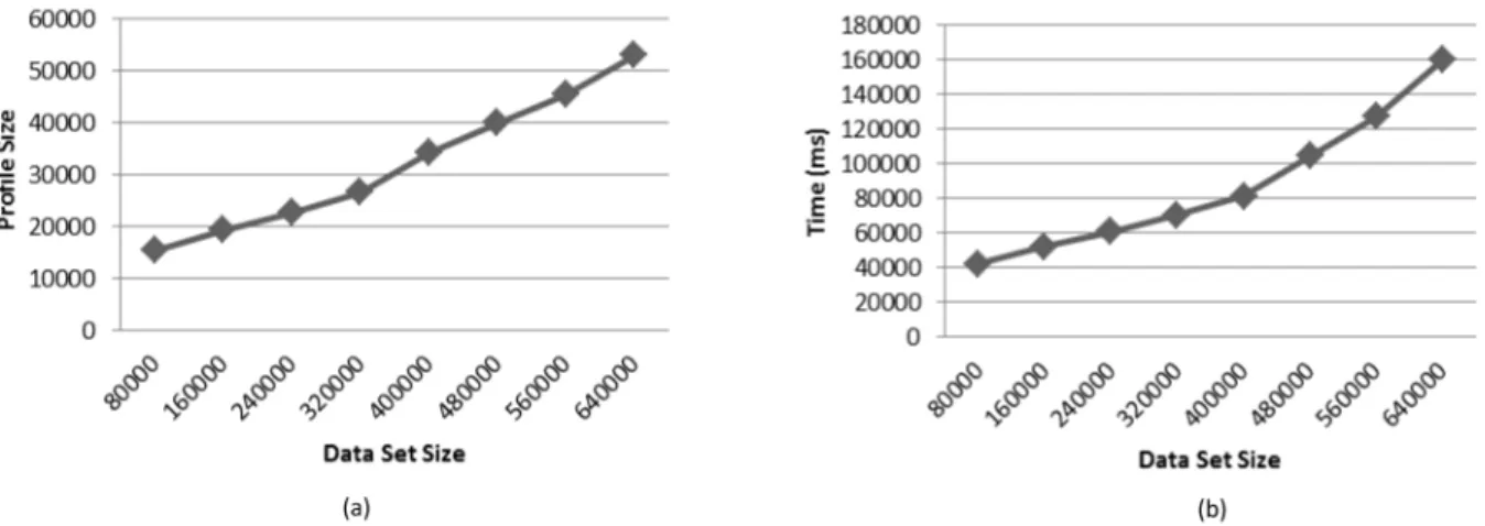
Figure 4.6: Scalability graphs (a) generated profile size versus data set size (b) profile generation
time vs database size
Effect of Input Data SizeFigure 4.6 illustrates the scalability of the proposed algorithms. We used a smaller sub set of DBLP dataset for our experiment and increased the size by selecting a larger subset each time until reaching the whole data set and for each experiment we create a new set of queries. Figure 4.6 illustrates the effect of data set size on the size of conditional DQ profile, it also illustrates the effect of data set size on the profile generation time. Experiments are ran with thresholds = 0.2 and τ = 20.
4.2
DQ Sample Trie Approach
Previous approach for generating conditional DQ profiles is best suitable when accuracy of DQ estimation is required for every query and enough resources and time is available to generate DQ measurements for every record of data. In environments where access to data and measurement and generation of DQ profile is costly (e.g. web or cloud applications) and some inaccuracy in estimated DQ can be acceptable, more flexible and more resource conserving techniques are required to generate conditional DQ profile. In web environment, amount of data that is available to the DQ Mediator (See Figure 2.1) is not pre-processable.
Amount of data that users query from DQ Mediator at every moment can also be over-whelming and varying time to time. However, due to the nature of DQ measurement, the DQS usually has limited power and can not process DQ for all the data that DQ Mediator is handling. For example DQS may be able to process accuracy of a few hundred addresses, or correctness of less than a hundred urls per second, but the amount of data that is pro-cessed by DQ Mediator can be easily tens of times more than the DQS limitations. In such case that DQS becomes a bottleneck an incremental cost-effective approach is required for creating DQ profiles.
DQ Profile Table estimates DQ of a given query by looking up the pre-processed estimate from the Profile Table. There is a very small overhead for every query, to store the DQ mea-surement value. However, the DQ meamea-surement value can not be re-used for other queries. Storing sample instead of DQ measurement value can let us re-use the DQ measurements made for previous queries to estimate DQ of the future queries. Re-using samples to answer different queries can drop the cost of DQ measurement (Unfortunately, samples can not guarantee the accuracy of estimation, so if the accuracy of estimation must be guaranteed, the Profile Table approach is more suitable).
In DQAQS, users and decision makers issue queries (to DQ Mediator) and if possible they will be immediately informed about the estimation of the quality of data they will receive as well as confidence level of the estimation. Then user can decide to continue with the query or take another action such as issuing another query. Sampling technique should be able to take advantage of fast local memory and storage of the mediator when it is available, but the limited resources should be utilized in a way that maximizes user satisfaction. Different
subsets of database have different popularity for the system’s users. For example prestigious database conferences are more queried by users of this particular system, hence there is more value in sampling respective subsets of database. Since external limitation define constrains on the cost, not all necessary samples can be generated. The system should decisively generate only samples that contribute the most to the final user satisfaction (i.e. accuracy of DQ estimation). For example if the only cost is the sample size, and 100 samples with a total size of 1000 rows are required to accurately estimate DQ for all the queries, but the cost restrictions do not allow for more than 100 sample rows, a portion of samples should be created that do not exceed 100 rows, and also the sum of popularity is being maximized.
Another aspect of a good sampling technique is provision of an accurate response even for queries that return small number of records while the overall size of samples is minimized. To achieve this aspect, biased sampling techniques [1] are suggested in literature. For DQ profiling, cost of measurement of DQ highly overweights the cost of storage (which is usually the most important cost for biased sampling techniques). Measuring DQ is inherently ex-pensive. For example correctness of an address requires a number of lookups in a data base and assurance of a web address requires calling the web address and parsing the returned page, etc. Therefore, we try to re-use parts of the sample to generate a more accurate DQ estimate with minimum extra cost.
For example if a Computer Science publication data set has 1000 records forJ IS journal papers, and 10 records for J IS papers of year 2011, a uniform 1% sample of JIS papers will include probably only one or zero sample records from 2011 JIS papers. If users show specific interest for recent JIS papers (i.e. popularity of the query) it makes sense to create
a small sample for 2011 JIS papers in addition to the 1% sample for all JIS papers. Once a dense sample like 2011 JIS papers is created, we will utilize it to enrich the DQ estimation for every query that may include data from this sample.
4.2.1
Sample Trie
We utilize a variation of suffix trie data structure (which we call sample trie) for accessing different samples from different subsets of data set. Figure 4.7 illustrates a sample trie for a given query workload.
Sample tree is a forest (set of disjoint trees) where each tree represents all samples that relate to a suffix of conjunctive selection conditions on attributes. For example, in Figure 4.7, attribute are year, venue, and university. Longest conjunctive selection condition on attributes consists of three selection conditions referring to all these three attributes. We assume a constant order in the presentation of attributes in conjunctive conditions (e.g. all selection conditions is assumed in the order of year, venue, university), hence, every single tree in the sample trie forms a suffix of this longest selection condition. The complete sample trie for this example wil consist of one tree of all conjunctive selection conditions made of year, venue, and university. Another tree for all conjunctive selection conditions made of venue, and university. Last tree for the selection conditions made of only university.
Each node of the trie that is marked with a number, represents a sample which is gen-erated as a uniform sample from the query response. Density of every sample in the trie may be different from others. For example sample 3, should represent a denser sample than sample 2. Assume sampling rate of both samples 3 and 2 are 0.1, which means for every 10
records in the query result, there is 1 record in the sample. If new query, year=2010 and venue=JIS and uni=UQ that returns 20 records is issued to the system, both samples 2 and 3 may contain only 2 records that satisfy the query conditions. In sample trie, each sample is denser than it’s parents in the trie. E.g. if sample 2 is created with uniform sampling rate of 0.1, sample 3 may be created with uniform sampling rate of 0.4, which means it may contain 8 records for above query. In the rest of this paper, we use the terms node and sample interchangeably for nodes of the trie and the sample they contain.
Query
1- Year between 2008 and 2012 & Venue = JIS 2- Year = 2010
3- Year = 2010 & Venue = JIS 4- Year = 2011
5- Venue = JIS
6- Venue = JIS & University = UQ 7- University = UQ Year=(2008-2012) Year=2010 Venue=JIS Venue=JIS Year=2011 Venue=JIS Uni=UQ Uni=UQ 3 4 1 5 6 7 2
Figure 4.7: Sample trie and a query workload
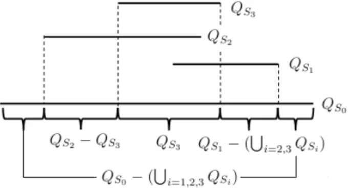
Nodes in the sample trie have the following characteristics: 1) Each sampleS represents a query SQ with selection condition as the conjunction of the node’s condition with it’s
parent’s conditions (recursively to the root node) 2) Each node is subset of its parent node. NodeS1 is subset of the nodeS2 if the query response forQS1 is subset of the query response for QS2. For illustration purpose, the sample trie of the Figure 4.7 represents one node for every query, however, various techniques in the rest of this section are suggested to use a much smaller sample tire (bound to cost limits) to estimate DQ accurately, for as many
queries as possible. Sample trie, differs from a suffix trie in the terms that not every suffix for one node’s query necessarily exists in the trie. Samples are created only when needed (e.g. Figure 4.7, query 7 is a suffix for query 6, but node 7 is only created when required. It is not created with node 6).
Sample trie can be used to estimate DQ of a given query. For uniform samples, the denser the sample is, it provides more accurate estimate for the given query. The benefit of a sample trie, is that if the lower density samples are not able to provide an accurate DQ estimation, there might be a denser sample that can help for finding a more accurate estimate. The sample trie can be generated to maximize the possibility of the queries being accurately estimated. To estimate DQ of a query result from a sample, we should first run the query against the sample. A query can be satisfied from a sample if running the query against the sample, returns enough number of records that can estimate DQ of the query results with some confidence. We define confidence of the DQ estimation, as max(1−1/|QS|, γS), where |QS| is the size of the query result ran against sample S and γS is the sampling rate.
Confidence of DQ estimation is related to the size of results returned from sample, but if the number of result is very low (e.g. 1) while sampling rate is very high (e.g. 1) the confidence reflects the sampling rate. User defines what confidence threshold is acceptable.
Assuming the sample trie exists, for a given query Q, there might be three possibilities where we might be able to use the sample trie to estimate DQ of the result of Q: 1) There exists at least one sample S that Q can be totally satisfied from (i.e. Q is subset ofS and
Q can be satisfied from S). In this case QS (result of running Q against S) provides an
estimation accuracy even further. 2) There is no sample that satisfies Q, but there are a number of samples that satisfy a part of Q, and there exists a sampleS that is a superset of the query (which is not dense enough to answerQwithin the confidence threshold, otherwise it would totally satisfy Q). In this case, an estimate of the DQ of the query result cannot be calculated, because sample trie does not have enough data to completely cover Q. For such situations, we provide a lower bound for the DQ estimation. 3) There is no sample that totally satisfies Qnor there is a sample that is superset ofQ. In this case, even a lower bound of DQ can not be estimated. Instead, we use all information available to provide a DQ estimate with unknown confidence.
Generation and utilization of the sample trie are not two distinct phases. In fact, the purpose of using sampling is to re-use the DQ metrics processed for a part of dataset, for as many queries as possible. Therefore, we integrate the algorithm for creation of the sample trie with its utilization. We employ popularity of the queries to identify their significance to the overall user satisfaction (i.e. DQ estimation accuracy). We consider two common scenarios, first, when the query workload is available in advanced. For example online systems that user pattern is predictable (e.g. users query pattern for one week is a good representation of the query pattern for next week). In this case we can provide a more cost effective sample and we can optimize the total cost more accurately. Second scenario, is when the query log can not be assumed in advanced (i.e. users querying pattern is totally unpredictable and varying). In this case, cost effectiveness can not be optimum, as we cannot predict user behaviour. Hence, we try improve the cost effectiveness based on the moving average of user querying pattern.
To define a sample tree, let N represent sample S, and N.Q represent the query that generates the sample for nodeN. For any N0 as a child of N,N0.Q⊆N.Q(We use existing view matching techniques [14] to identify if a query is subset of another query).
Let A be set of attributes ai and |Dai| be size of the value domain of each attribute ai.
Imagine the longest conjunctive selection condition that includes all ai in the order of|Dai|
(For example attributes Y ear,Domain, andV enueare in order of|Dai|). The suffix trie for the longest conjunctive selection condition illustrates the sample trie that will be resulted if all possible samples are generated. Creating the suffix trie in order of |Dai| helps to reduce
the bushiness of this trie which makes it easier to maintain. Therefore, we organize each conjunctive selection conditions in the order of |Dai|and we create the suffix trie using this
order. Each node of the sample trie contains the sample for the query, a list of child samples, and other meta-data like density of the sample and popularity of the sample’s query which are describe later.
4.2.2
Sample Trie Algorithm
We assume that a constant or recurring limit for all different costs such as memory, storage, and DQS access is provided. Following steps define the general framework for creating the sample trie from the query workload. Inputs are: query Q0 with popularity ρ, and DQ sample trie T. We consider popularity as the number of times a query is issued by users.
1. Find the deepest node N in trie T whereQ0 ⊆N.Q.
2. If N Satisfies estimation of DQ for Q0, then returnEstimation of DQ for Q0
4. If it is Worthy to create a new sample for Q0, then create the new sample S0, and populate the DQ metrics by running it against DQS. Create a new node N0 assigned to sample S0, query Q0 and popularity ρ and add it to the trie as child of N. All children of N should then be reorganized to keep the trie valid. (e.g. if any node is subset of N0 should be moved underN0)
The above algorithm provides a general framework for definition of the various approaches in this paper. Every approach we define works in the context of the above algorithm, but each approach provides a different definition for at least one of the functions in the algorithm, presented in italic. There are three key functions in the above framework, namely;
Satisfaction, DQ Estimation, andWorthiness. We provide basic and cost-based approaches. Basic and naive approaches provide minimum functionality for all functions of the above algorithm, and cost-based approach will re-define the worthiness and estimation functions to make the above algorithm cost-effective. Eventually we re-define the estimation function from the cost-based approach to maximize the accuracy of DQ estimation based on all data available in the sample trie. Below, we define the discussed approaches in more detail:
a-Naive Approach Easiest approach to build a sample tire, is to create one sample per
distinct query as long as the costs are not overflown. To implement this approach we will define the algorithm functions as follows: Satisfaction, A query is only satisfied with a node if the node represents the same query. DQ Estimation, DQ can be estimated by running the query against the sample. Worthiness, every new query is worthy of creating a new sample (worthiness function returns true regardless of the query).