"As You Sow So Shall You Reap: From Capabilities to Opportunities"

(1)

Working Paper No. 613

As You Sow So Shall You Reap:

From Capabilities to Opportunities

by

Jesus Felipe Utsav Kumar Arnelyn Abdon

Asian Development Bank, Manila, Philippines*

August 2010

* This paper represents the views of the authors and not those of the Asian Development Bank, its executive directors, or the member countries they represent. Contacts: jfelipe@adb.org (corresponding author); ukumar.consultant@adb.org; aabdon.consultant@adb.org.

The Levy Economics Institute Working Paper Collection presents research in progress by Levy Institute scholars and conference participants. The purpose of the series is to disseminate ideas to and elicit comments from academics and professionals.

Levy Economics Institute of Bard College, founded in 1986, is a nonprofit, nonpartisan, independently funded research organization devoted to public service. Through scholarship and economic research it generates viable, effective public policy responses to important economic problems that profoundly affect the quality of life in the United States and abroad.

Levy Economics Institute P.O. Box 5000

Annandale-on-Hudson, NY 12504-5000 http://www.levyinstitute.org

(2)

1

ABSTRACT

We develop an Index of Opportunities for 130 countries based on their capabilities to undergo structural transformation. The Index of Opportunities has four dimensions, all of them

characteristic of a country’s export basket: (1) sophistication; (2) diversification; (3)

standardness; and (4) possibilities for exporting with comparative advantage over other products. The rationale underlying the index is that, in the long run, a country’s income is determined by the variety and sophistication of the products it makes and exports, which reflect its accumulated capabilities. We find that countries like China, India, Poland, Thailand, Mexico, and Brazil have accumulated a significant number of capabilities that will allow them to do well in the long run. These countries have diversified and increased the level of sophistication of their export

structures. At the other extreme, countries like Papua New Guinea, Malawi, Benin, Mauritania, and Haiti score very poorly in the Index of Opportunities because their export structures are neither diversified nor sophisticated, and they have accumulated very few and unsophisticated capabilities. These countries are in urgent need of implementing policies that lead to the accumulation of capabilities.

Keywords: Capabilities; Index of Opportunities; Diversification; Open Forest; Product Space; Sophistication; Standardness

JEL Classifications: O10, O57

(3)

1. INTRODUCTION

The past 20 years have seen the rise of developing countries and their contribution to world GDP growth has increased significantly. The share of these countries in world growth has increased from around 45% in 1990–2000 to almost 60% in the last decade. Among the developing economies, a great deal of attention has been paid to the so-called BRIC countries, Brazil, Russia, India, and China (Wilson and Purushothaman 2003). China and India have seen the fastest growth. However, given their respective per capita incomes of $5,000 and $2,600 (in 2005 PPP$), both are still far from the advanced countries. Brazil and Russia, with per capita incomes of $8,000 and $13,000, are closer tothe advanced countries. Whether these four economies will eventually catch-up with the high-income countries will depend on their ability to continue, and to the extent possible accelerate, the pace of structural transformation of their economies.

Structural transformation is the process through which countries change what they produce and how they do it. It involves a shift in the output and employment structures away move from low-productivity and low-wage activities into high-productivity and high-wage activities; as well as the upgrading and diversification of their production and export baskets. This process generates sustained growth and enables countries to increase their income per capita.

In recent research, Hidalgo et al. (2007) and Hausmann, Hwang, and Rodik (2007) argue that while growth and development are the result of structural transformation, not all activities have the same implications for a country’s growth prospects. They show that the composition of a country’s export basket has important consequences for its growth prospects. Hidalgo et al. (2007) argue that development should be understood as a process of accumulating more complex sets of capabilities (e.g., bridges, ports, highways, norms, institutions, property rights,

regulations, specific labor kills, laws, social networks) and of finding paths that create incentives for those capabilities to be accumulated and used (Hidalgo 2009; Hidalgo and Hausmann 2009). The implication is that a sustainable growth trajectory must involve the introduction of new goods and not merely involve continual learning on a fixed set of goods. They summarize this idea in the newly developed product space.

(4)

2

In this paper, we develop a new “Index of Opportunities” based on a country’s

accumulated capabilities to undergo structural transformation. It captures the potential for further upgrading, growth, and development. The Index of Opportunities has four dimensions, all related to a country’s export basket and its position in the product space: (i) its sophistication; (ii) its diversification; (iii) its standardness; and (iv) the possibilities that it offers for a country to export other products with comparative advantage. The idea underlying the index is that, in the long run, a country’s income is determined by the variety and sophistication of the products it makes and exports, and by the accumulation of new capabilities.1

The rest of the paper is structured as follows. Section 2 provides a summary of Hidalgo et al’s. (2007) product space, and explains the rationale underlying the Index of Opportunities. Sections 3 through 6 delve into the dimensions of the index, and section 7 shows how it is constructed. We find that China and India are the top-ranked countries among the non-high-income countries (a total of 96 countries).2 Poland, Thailand, Mexico, and Brazil are next, while Russia is ranked 18th, with a significantly lower index. Other Asian countries ranked high are: Indonesia (8th), Malaysia (10th), the Philippines (13th), Vietnam (21st), and Georgia (29th). In section 8, we analyze and discuss the product space of some non-high-income countries that are ranked high according to our Index of Opportunities and compare it with that of Germany. Section 9 concludes the paper.

2. THE PRODUCT SPACE

According to conventional trade theory, countries export products that use intensively those factors of production in which they are relatively abundant. Thus, the patterns of specialization are uniquely determined by the factor endowments, independently of initial conditions. On the other hand, the new trade theory argues that patterns of specialization cannot be determined independently of initial conditions. In recent work, Hausmann, Hwang, and Rodik (2007) argue that specialization patterns are indeterminate and may be shaped by idiosyncratic elements. They show that there is a positive relationship between the growth prospects of a country and the

1

Chang (2009) argues that development is largely about the transformation of the productive structure and the capabilities that support it. This is what the index tries to capture.

2

(5)

sophistication level of the country’s export basket. One implication of this relationship is that for countries to undergo structural transformation and grow, their export baskets must continuously evolve, and the share of sophisticated exports should increase.

A country’s ability to foray into new products depends on whether the set of existing capabilities necessary to produce these products (human and physical capital, legal system, institutions, etc.) can be easily redeployed for the production and export of new products. These existing capabilities reflect the package that the country produces and exports with comparative advantage. For example, it is probably easier for a country that exports T-shirts to add shorts to its export basket than to add smart phones. On the other hand, it is very likely that a country that exports basic cell phones has the capabilities to add smart phones to its export basket. This implies that it is easier to start producing a “nearby” product (in terms of required capabilities to export it successfully) than a product that is “far away,” which requires capabilities that the country probably does not possess. Hidalgo et al. (2007) conceptualize these ideas in the newly developed product space.

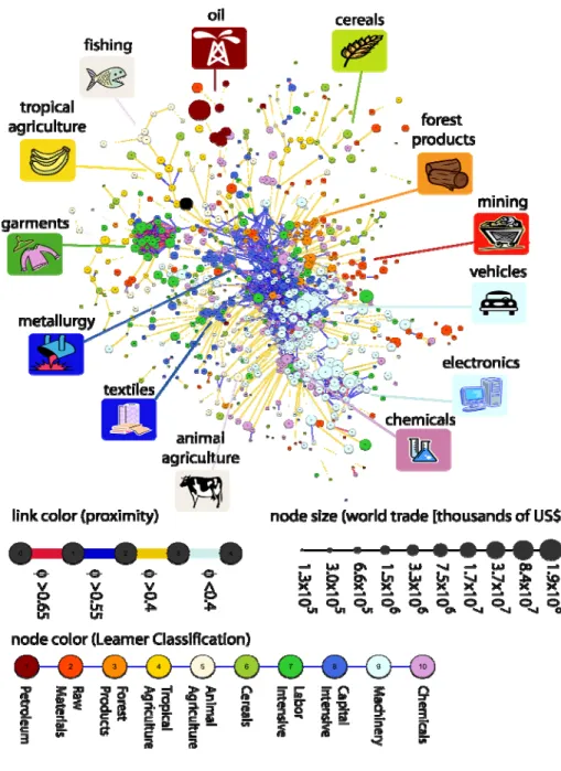
The product space is an application of network theory that yields a graphical

representation of all products exported in the world. The main aspect of this representation is that it shows the “proximity” of all products. Figure 1 shows the product space. The different circles represent products (a total of 779 in our analysis). The size of the circles is proportional to their share in total world trade. Colors represent the ten different product groups based on Leamer’s classification (Leamer 1984). 3 The lines linking the circles represent the proximity between them. Proximity in this context is not a physical concept; rather, it measures the likelihood that a country exports a product given that it exports another one. A red line indicates a high

probability of exporting both products with comparative advantage, while a light blue line indicates a low probability that the two products are exported jointly. The rationale is that if two goods need similar capabilities, a country should show a high probability of exporting both with comparative advantage.

We can see that the product space is highly heterogeneous. Some products are close-by to others (because they require similar capabilities), while some others are in a sparse area of the product space. In the first case, it easy to jump from one product into another one (and therefore

3

The products are categorized according to the Leamer Classification (Leamer 1984). See appendix table 1 for Leamer Classification.

(6)

4

exporting it with comparative advantage), while in the second case it is difficult. The core of the product space—the area with many products close by—comprises chemicals, machinery, and metal products (320 products, 41% of the total). The periphery consists of petroleum, raw materials, tropical agriculture, animal products, cereals, labor intensive goods, and capital intensive goods (excluding metal products).

The heterogeneous structure of the product space has important implications for structural change. If a country exports goods located in a dense part of the product space, then expanding to other products is much easier because the set of already acquired capabilities can be easily redeployed for the production of other nearby products. This is likely to be the case of different types of machinery or of electronic goods. However, if a country specializes in the peripheral products, this redeployment is more challenging as no other set of products requires similar capabilities. This is the case of natural resources such as oil. A country’s position within the product space, therefore, signals its capacity to expand to more sophisticated products, thereby laying the groundwork for future growth.

(7)

Figure 1: The Product Space

Source: Hidalgo et al. (2007)

A country’s export basket can be described according to the following characteristics: (i) its sophistication; (ii) its diversification; (iii) its standardness; and (iv) possibilities to export other products with comparative advantage.

The level of sophistication of the export basket captures its income content. It is

(8)

6

calculated as a weighted average of the GDP per capita of the countries that export a given product. Therefore, a high level of sophistication indicates that the export basket is similar to that of the rich countries. Hausmann, Hwang, and Rodik (2007) show that countries with a more sophisticated export basket grow faster. We also look at the sophistication level of the products in the “core” of the product space. Countries with a high sophistication level in the core of the product space have acquired more complex capabilities, which will make it easier to export even more sophisticated products.

The diversification of a country’s export basket is measured by the number of products in which the country has acquired revealed comparative advantage. Diversification measures the country’s ability to become competitive in a wider range of products. The rationale that underlies our analysis is that technical progress and structural change evolve together (technical progress induces structural change and vice versa; they jointly lead to growth), and underlying both is the mastering of new capabilities. An additional aspect of diversification that we look at is the number of “core” commodities that a country exports with comparative advantage. This is an indicator of the range of capabilities that a country has acquired in the core of the product space. Products in the core are, on average, more sophisticated than outside the core and have many other products nearby, which offers the possibility of acquiring comparative advantage in them (because they are nearby, a country already has some of the required capabilities to export them successfully). It might be the case that two countries are equally diversified, but, other things equal, the one that exports more core commodities with comparative advantage will be better off to continue diversifying. The reverse might also be true: two countries may have comparative advantage in a similar (absolute) number of products in the core, but in one case, the number of core commodities exported with comparative advantage might represent a greater share of the total number of commodities exported with comparative advantage. It may be difficult for a small country to export as many products as a large country (e.g., Switzerland, Singapore, or Ireland). However, this country may have a very sophisticated basket. We account for this factor by incorporating in the index the ratio of the number of core commodities exported with

comparative advantage to the total number of commodities exported with comparative advantage.

(9)

Another aspect of the export basket is its uniqueness, i.e., how many countries are producing the same product. This measure of uniqueness of the export basket has been called “standardness” (Hidalgo and Hausmann 2009).

The final factor that enters the Index of Opportunities is a measure of the potential for further structural change, called open forest. In a recent paper, Hausmann, Rodriguez, and Wagner (2008) conclude that countries with a higher open forest are better prepared to react successfully to adverse export shocks. Open forest is a summary measure of how far the products still not exported with comparative advantage are from the current export basket.

3. EXPORT SOPHISTICATION

The first two factors that we consider in the Index of Opportunities are the sophistication level of the overall export basket (denoted EXPY) and the sophistication level of the core products (denoted EXPY-core).

The sophistication level of the export basket (EXPY) of a country captures its ability to export products produced and exported by the rich countries, to the extent that, in general, the exports of rich countries embody higher productivity, wages, and income per capita. The level of sophistication of a country’s export basket is calculated as the weighted average of the

sophistication of the products (PRODY) exported.4

4

Following Hausmann, Hwang, and Rodik (2007), we calculate the level of sophistication of a product (PRODY) as a weighted average of the GDP per capita of the countries exporting that product. Algebraically:

ci ci i i c c ci ci c i xval xval PRODY GDPpc xval xval ⎡ ⎤ ⎢ ⎥ ⎢ ⎥ ⎢ ⎥ = _⎢ _⎥× ⎛ ⎞ ⎢ _⎜ _⎟⎥ ⎢ _⎜ _⎟⎥ ⎢ _⎝ _⎠⎥ ⎣ ⎦

∑

_∑

(1)

where xvalci is the value of country c’s export of commodity i and GDPpcc is country c’s per capita GDP. PRODY is measured in 2005 PPP $. PRODY is then used to compute EXPY as:

(10)

8

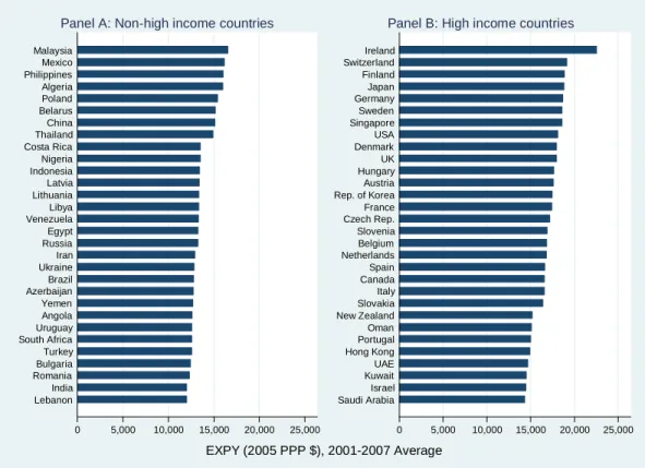
Figure 2 shows the top thirty countries in terms of EXPY (average of 2001–07). Panel A shows the non-high-income countries and panel B the high-income.5 In general, the export basket of the high-income countries is more sophisticated. Malaysia had the highest EXPY during 2001–07, followed by Mexico and Philippines. The sophistication level of China’s export basket was around $9,000–$10,000 in the 1960s (not shown) and increased to $15,159 during 2001–07. On the other hand, India’s average export sophistication during 2001–07 was $12,005, and ranked 29th among the non-high-income countries. Both China and India have seen a significant increase in the sophistication level of their export baskets over the last 15 years (figure 3). On the other hand, the sophistication level of the export baskets of both Brazil and Russia has been constant in the $12,000 –$13,000 range over the last 15 years. While export sophistication is observed to remain constant in the high-income countries as well, this happens at much higher levels of sophistication.

∑ ∑

⎟⎟ ⎟ ⎠ ⎞ ⎜ ⎜ ⎜ ⎝ ⎛ × = i i i ci ci c PRODY xval xval EXPY (2) EXPY is measured in 2005 PPP$.

We use highly disaggregated (SITC-Rev.2 4-digit level) trade data for the years 1962–2007. Data from 1962–2000 is from Feenstra et al. (2005). This data is extended to 2007 using the UNCOMTRADE database. PRODY is calculated for 779 products. PRODY used is the average of the PRODY of each product in the years 2003–05. GDP per capita (measured in 2005 PPP$) is from the World Development Indicators.

5

(11)

Figure 2: Export Sophistication (EXPY), Average 2001–07 0 5,000 10,000 15,000 20,000 25,000 Lebanon India Romania Bulgaria Turkey South Africa Uruguay Angola Yemen Azerbaijan Brazil Ukraine Iran Russia Egypt Venezuela Libya Lithuania Latvia Indonesia Nigeria Costa Rica Thailand China Belarus Poland Algeria Philippines Mexico Malaysia

Panel A: Non-high income countries

0 5,000 10,000 15,000 20,000 25,000 Saudi Arabia Israel Kuwait UAE Hong Kong Portugal Oman New Zealand Slovakia Italy Canada Spain Netherlands Belgium Slovenia Czech Rep. France Rep. of Korea Austria Hungary UK Denmark USA Singapore Sweden Germany Japan Finland Switzerland Ireland

Panel B: High income countries

EXPY (2005 PPP $), 2001-2007 Average

Figure 3: Trend in Export Sophistication

8,000 10,000 12,000 14,000 16,000 18,000 20,000 E XPY (2 0 0 5 PPP $ ) 1992 1994 1996 1998 2000 2002 2004 2006 Brazil Russia India PRC USA Japan Germany Rep. of Korea

(12)

10

Figure 4: GDP Per Capita, Average 2001–07

0 10,000 20,000 30,000 40,000 50,000 Peru Dominican Rep. Tunisia Ecuador Algeria Jamaica Colombia Macedonia Belarus Kazakhstan South Africa Brazil Bulgaria Costa Rica Romania Panama Iran Uruguay Lebanon Venezuela Turkey Argentina Russia Malaysia Chile Latvia Mexico Libya Lithuania Poland

0 10,000 20,000 30,000 40,000 50,000 Czech Rep. Saudi Arabia Portugal Rep. of Korea Slovenia Israel New Zealand Greece Spain Italy Japan Finland France Australia Sweden Germany UK Belgium Denmark Austria Hong Kong Canada Netherlands Switzerland Ireland Kuwait USA Singapore UAE Norway

GDP per capita (2005 PPP $), 2001-2007 Average

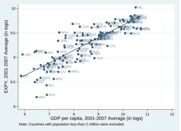
Comparing the sophistication level of the export baskets with the corresponding per capita incomes (figure 4, panel A), we find that countries such as China, Indonesia, and the Philippines have higher export sophistication levels than those of Brazil and Russia, but the latter have higher per capita incomes.6 India’s export sophistication ($12,005) is not significantly different from that of Brazil ($12,836) or from Turkey’s ($12,549). The latter two, however, have higher per capita incomes. Figure 5 shows the relationship between sophistication and income per capita. Countries such as China, India, Indonesia, or the Philippines have a more sophisticated export basket than would be expected given their level of development (proxied by per capita income).7 Among other countries that have a higher than expected sophistication level given their per capita income are Algeria, Egypt, Malaysia, Nigeria, Poland, and Thailand. On

6

The average (for the period 2001–07) per capita incomes (measured in 2005 PPP$) of China ($3,823), India ($2,122), Indonesia ($3,100), and the Philippines ($2,846) are not even in the top 30 and therefore are not shown in the chart.

7

(13)

the other hand, Brazil, Russia, and the advanced countries are closer to the sophistication levels that would be expected for countries in their respective income categories.

To stress the significance of the point made in the previous paragraph, note that the per capita income of today’s rich countries when they had levels of export sophistication similar to those of China and India in 2007 was much higher. For example, Japan’s (Korea’s)

sophistication level in the late 1970s (mid-1990s) was similar to China’s sophistication level today, but the per capita income in Japan (Korea) at the time was $17,000 ($16,000), more than three times that of China in 2007, roughly $5,000 (measured in PPP, 2005 prices). Similarly, Korea’s EXPY in the year 1985 was comparable to that of India in 2007, but at three times the per capita income (Korea’s per capita income in 1985 was $7,500 and India’s per capita income in 2007 was $2,600).

Figure 5: EXPY and GDP Per Capita, Average 2001–07

AGO ALB ARE ARG ARM AUS AUT AZE BDI BEL BEN BFA BGD BGR BIH BLR BOL BRA CAF CAN CHE CHL CHN CIV CMR COG COL CRI CZE DEU DNK DOM DZA ECU EGY ESP ETH FIN FRAGBR GEO GHA GIN GRC GTM HKG HND HRV HTI HUN IDN IND IRL IRN ISR ITA JAM JOR JPN KAZ KENKGZ KHM KOR KWT LAO LBN LBR LBY LKA LTU LVA MAR MDA MDG MEX MKD MLI MNG MOZ MRT MWI MYS NER NGA NIC NLD NOR NPL NZL OMN PAK PAN PER PHL PNG POL _PRT PRY ROM RUS RWA SAU SDN SEN SGP SLE SLV SVK SVN SWE SYR TCD TGO THA TJK TKM TUN TUR TZA UGA UKR _URY USA UZB VEN VNM YEM ZAF ZMB 8 8.5 9 9.5 10 EXPY, 2 0 0 1 -2 0 0 7 Ave ra g e (i n l o g s ) 6 7 8 9 10 11 12

GDP per capita, 2001-2007 Average (in logs)

(14)

12

Felipe (2010: table 10.4) estimates that a 10% increase in EXPY at the beginning of the period raises growth by about half a percentage point. From this perspective, the sophistication level of the export basket of some of the lower- and middle-income countries, such as China, India, Indonesia, Thailand, or the Philippines gives them a greater chance of rapid growth in the coming years.

A second indicator of sophistication that we examine is the sophistication level of the exports that belong to the core of the product space. We call this EXPY-core. This is calculated as overall EXPY (equation 2), except that the set of commodities over which sophistication is measured is restricted to the core of the product space: machinery, chemicals, and metals. Core commodities are significantly more sophisticated than commodities outside the core: average PRODY of the core is $18,687, while it was $11,634 for products outside the core.

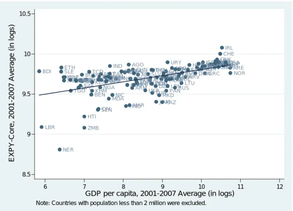
Figure 6 shows the average sophistication level of the core exports for the period 2001– 07. Among the non-high-income countries with the highest sophistication of the core exports, Uruguay’s core exports are the most sophisticated, followed by Angola’s and India’s. It is worth noting that not only does the ranking change, but also the composition of the top 30 countries, when compared with the overall export sophistication (figure 2). For example, Bangladesh and Pakistan, which were not in the top 30 in terms of overall export sophistication (figure 2, panel A), are in the top 30 when we consider the sophistication of the core exports (figure 6, panel A). Similarly, Argentina, which is just outside top 30 in terms of overall export sophistication, is in the top 10 when we consider the sophistication of the core exports. China’s core exports are less sophisticated than India’s, though the difference is small.

The average sophistication level of India’s core exports ($18,955) during 2001–07 is similar to that of France ($19,300), Japan ($19,288), Spain ($19,258), Hong Kong ($18,750), Australia ($18,665), and Korea ($18,308). The latter, however, have much higher income levels than India.

(15)

Figure 6: Sophistication of the Core (EXPY-core), Average 2001–2007 0 5,000 10,000 15,000 20,000 25,000 Iran Tajikistan South Africa Bangladesh Azerbaijan Libya El Salvador Mauritania Pakistan Syria Brazil Poland Indonesia Chad Sierra Leone Philippines Burundi Congo Costa Rica Sri Lanka Ecuador Thailand China Mexico Malaysia Argentina Ethiopia India Angola Uruguay

0 5,000 10,000 15,000 20,000 25,000 Slovakia Portugal Rep. of Korea UAE Australia Czech Rep. Hong Kong Slovenia New Zealand Kuwait Canada Finland Austria Hungary Spain Japan France Italy Saudi Arabia Singapore Sweden Belgium USA Netherlands Israel Germany UK Denmark Switzerland Ireland

EXPY-Core (2005 PPP $), 2001-2007 Average

Figure 7 plots the sophistication level of the core exports against per capita income. In general, countries at a higher stage of development have more sophisticated export baskets, but it is worth noting that given their per capita incomes, the sophistication levels of Angola’s, India’s, China’s, and Uruguay’s core-exports is greater than what one would expect. On the other hand, the sophistication of Brazil’s core exports is close to what one would expect for a country at its stage of development, while Russia’s is below the average.

(16)

14

Figure 7: EXPY-core and GDP Per Capita, Average 2001–07

AGO ALB ARE ARG ARM AUSAUT AZE BDI BEL BEN

BFABGD BOL BIH BLRBGR

BRA CAF CAN CHE CHL CHN CIV CMR COG COL CRI CZE DEUDNK DOM_DZA ECU EGY ESP

ETH FINFRA

GBR GEO GHA GIN GRC GTM HKG HND HRV HTI HUN IDN IND IRL IRN ISRITA JAM JOR JPN KAZ KENKGZ KHM KOR KWT LAO LBN LBR LBY LKA LTU LVA MAR MDA MDG MEX MKD MLI MNG MOZ MRT MWI MYS NER NGA NIC NLD NOR NPL NZL OMN PAK PAN PER PHL PNG POL PRT PRY ROM RUS RWA SAU SDN SEN SGP SLE _SLV SVK SVNSWE SYR TCD TGO THA TJK TKM TUN TUR TZA UGA UKR URY USA

UZBVNMYEM VEN

ZAF ZMB 8.5 9 9.5 10 10.5 EXPY-C o re , 2 0 0 1 -2 0 0 7 Av e ra g e (i n l o g s ) 6 7 8 9 10 11 12

GDP per capita, 2001-2007 Average (in logs)

Note: Countries with population less than 2 million were excluded.

This exercise indicates that the sophistication level of the export basket, and therefore the implicit accumulated capabilities, differs across countries. This is due to the different types of products exported. This brings us to the following question: do countries differ in the number of products exported with comparative advantage?

4. DIVERSIFICATION

A key insight from Hidalgo et al. (2007) is that the more diversified a country, the greater are its capabilities, which allows it to acquire comparative advantage in other products. In this paper,

diversification is measured by the absolute number of products that a country exports with comparative advantage. Revealed comparative advantage (RCA) is measured as the ratio of the

(17)

export share of a given product in the country’s export basket to the same share at the world level.8

Figure 8 shows the average diversification of the export basket, over the period 2001– 07.9 During this period, China and India exported 257 and 246 products, respectively with comparative advantage. Except for Indonesia (which exported 213 products with comparative advantage) and Thailand (197 products), no other lower-middle income had a comparative advantage in so many products. Other countries so diversified were either upper-middle income countries such as Poland (265), Turkey (235), Bulgaria (214), Romania (194), or Lithuania (192); high-income non-OECDcountries such as Slovenia (226) or Croatia (204); or high-income OECD countries such as Germany (340), Italy (325), United States (318), France (315), Spain (300), Belgium (278), Czech Republic (270), Austria (262), Great Britain (244),

Netherlands (233), Denmark (216), or Japan (200). Korea had comparative advantage in 154 products during the period 2001–07. Brazil and Russia, both upper-middle income countries, exported 190 and 105 products, respectively, with comparative advantage.

Figure 9 shows that both China and India are positive outliers in the sense that their export baskets are more diversified than one would expect given their income levels. Indonesia, Poland, and Turkey are other non-high-income countries that are positive outliers. Brazil is also above the fitted line; Russia, on the other hand, has comparative advantage in fewer products than would be expected given its income level.

8_{We use the measure proposed by Balassa (1965), Algebraically:}

∑∑

∑

= i c ci c ci i ci ci ci xval xval xval xval RCA (3)

A country c is said to have revealed comparative advantage (RCA) in a commodity i if the above-defined index,

RCAci, is greater than 1. The index of revealed comparative advantage can be problematic, especially if used for comparison of different products. For example, a country very well endowed with a specific natural resource can have a RCA in the thousands. However, the highest RCA in automobiles is about 3.6.

9

Measure of diversification shown is the average number of products that a country exported with revealed comparative advantage during 2001–07. It does not show that a country, say China, had revealed comparative advantage in the same 257 products in each year during 2001–07.

(18)

16

Figure 8: Diversification, Average 2001–07

0 50 100 150 200 250 300 350 Peru Uruguay Jordan Macedonia Panama Kenya Pakistan Guatemala Bosnia Colombia Tunisia Mexico Viet Nam Belarus Egypt Lebanon Argentina Latvia Ukraine Brazil Lithuania Romania Thailand South Africa Bulgaria Indonesia Turkey India China Poland

0 50 100 150 200 250 300 350 Ireland Norway Singapore Australia New Zealand Israel Rep. of Korea Finland Hong Kong Hungary Slovakia Japan Portugal Croatia Canada Switzerland Sweden Greece Denmark Slovenia Netherlands UK Austria Czech Rep. Belgium Spain France USA Italy Germany

(19)

Figure 9: Diversification and GDP Per Capita, Average 2001–07 AGO ALB ARE ARG ARM AUS AUT AZE BDI BEL BEN BFA BGD BGR BIH BLR BOL BRA CAF CANCHE CHL CHN CIV CMR COG COL CRI CZE DEU DNK DOM DZA ECU EGY ESP ETH FIN FRA GBR GEO GHA GIN GRC GTM HKG HND HRV HTI HUN IDN IND IRL IRN ISR ITA JAM JOR JPN KAZ KEN KGZ KHM KOR KWT LAO LBN LBR LBY LKA LTU LVA MAR MDA MDG MEX MKD MLI MNG MOZ MRT MWI MYS NER NGA NIC NLD NOR NPL NZL OMN PAK PAN PER PHL PNG POL PRT PRY ROM RUS RWA SAU SDN SEN SGP SLE SLV SVK SVN SWE SYR TCD TGO THA TJK TKM TUN TUR TZA UGA UKR URY USA UZB VEN VNM YEM ZAF ZMB 0 100 200 300 400 Di v e rs if ic at io n, 2 0 0 1 -2 0 0 7 A v er a g e 0 10,000 20,000 30,000 40,000 50,000

Figure 10 shows the average number of commodities in the core of the product space that countries exported with comparative advantage during 2001–07. On average, China exported 89 products with comparative advantage, India 81. Other lower-middle income countries where a large number of core commodities were exported with comparative advantage are Ukraine (73), Thailand (68), and Indonesia (45). Other countries that have comparative advantage in as many products in the core are either high-income (OECD and non-OECD) countries, or are upper-middle-income countries. Brazil exported 73 products in the core with comparative advantage, Russia only 44. For the high-income countries (those in the OECD) it is not uncommon to have comparative advantage in over 100 core commodities. The average number of products with comparative advantage in the core for the high-income OECD countries is 105.

(20)

18

Figure 10: Diversification-core, Average 2001–07

0 50 100 150 200 250 Georgia Costa Rica Senegal Macedonia Egypt Colombia Philippines Tunisia Bosnia Jordan Panama Argentina Russia Lebanon Indonesia Latvia Lithuania Malaysia Belarus Turkey South Africa Thailand Bulgaria Ukraine Brazil Romania Mexico India China Poland

0 50 100 150 200 250 Australia New Zealand Ireland Norway Hong Kong Greece Portugal Canada Croatia Singapore Hungary Israel Slovakia Rep. of Korea Finland Denmark Netherlands Slovenia Belgium Spain Sweden Czech Rep. Switzerland UK Austria Japan Italy France USA Germany

Diversification-Core, 2001-2007 Average

Finally, figure 11 shows that, given per capita income, China and India stand out in terms of number of core products exported with comparative advantage. Brazil, Mexico, Poland, Romania, and Ukraine also stand out in their income group, whereas Russia is close to the fitted line. Oil-rich countries such as Kuwait and Oman, which have a high level of export

(21)

Figure 11: Diversification-core and GDP per Capita, Average 2001–07 AGO ALB ARE ARG ARM AUS AUT AZE BDI BEL BEN BFA BGD BGR BIH BLR BOL BRA CAF CAN CHE CHL CHN CIV CMRCOG COL CRI CZE DEU DNK DOM DZA ECU EGY ESP ETH FIN FRA GBR GEO GHA GIN GRC GTM HKG HND HRV HTI HUN IDN IND IRL IRN ISR ITA JAM JOR JPN KAZ KENKGZ KHM KOR KWT LAO LBN LBR LKA LBY LTU LVA MAR MDA MDG MEX MKD MLI MNG MOZ MRT MWI MYS NER NGANIC NLD NOR NPL NZL OMN PAK PAN PER PHL PNG POL PRT PRY ROM RUS RWA SAU SDN SEN SGP SLE SLV SVK SVN SWE SYR TCD TGO THA TJK TKM TUN TUR TZA UGA UKR URY USA UZB VEN VNM YEM ZAF ZMB 0 50 100 150 200 Di v e rs if ic at io n -C o re , 20 01 -2 0 0 7 A v e rag e 0 10,000 20,000 30,000 40,000 50,000

The above discussion has highlighted the role of the size and nature of capabilities, measured by the number of products exported with revealed comparative advantage, both overall and core products. However, it may be the case that two countries export a similar number of products with comparative advantage, but the nature of the products differs, i.e., one of them has comparative advantage in a greater number of core products. For example, Great Britain and Turkey have comparative advantage in a similar number of products, 244 and 235, respectively. However, in the case of Great Britain, of the 244 products exported with comparative advantage, 139 lie in the core; whereas in the case of Turkey, only 60 out of the 235 lie in the core. Thus, the capabilities in the two countries are of a very different nature. A greater share of Great Britain’s capabilities seems to be of a more complex nature.

Similarly, two countries might have comparative advantage in a similar number of core products, but they might differ in the total number of products in which they have comparative advantage. For example, India and Korea export a similar number of core products with

(22)

20

comparative advantage, 81 and 85, respectively. This might seem to indicate that both have similar complex capabilities. However, the overall comparative advantage in the two countries is quite different. India has a comparative advantage in 246 products, while Korea in only 155 products. However, in the case of Korea, 85 are in the core, while in the case of India only 81 are in the core, i.e., a smaller share. Thus, Korea has a greater share of complex capabilities.

We account for this in the construction of our index by including the number of

commodities with revealed comparative advantage in the core as a ratio of the total number of commodities in which that country has a comparative advantage. We call this the share-core.

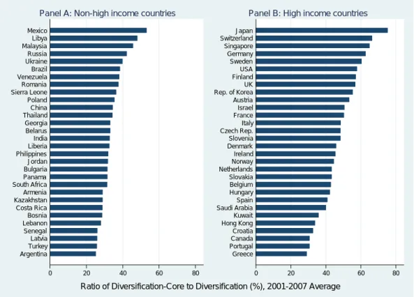
Figure 12 provides a comparison of share-core for non-high- and high-income countries. In general, high-income countries have a larger share of commodities exported with comparative advantage in the core (an average of 45%) than non-high-income countries (an average of 21%). In the case of non-high-income countries, Mexico stands out with a share of 53% of commodities exported with comparative advantage being in the core of the product space. Is this unusual for a country like Mexico given its per capita income?

Figure 12: Share-core, Average 2001–07

0 20 40 60 80 Argentina Turkey Latvia Senegal Lebanon Bosnia Costa Rica Kazakhstan Armenia South Africa Panama Bulgaria Jordan Philippines Liberia India Belarus Georgia Thailand China Poland Sierra Leone Romania Venezuela Brazil Ukraine Russia Malaysia Libya Mexico

0 20 40 60 80 Greece Portugal Canada Croatia Hong Kong Kuwait Saudi Arabia Spain Hungary Belgium Slovakia Netherlands Norway Ireland Denmark Slovenia Czech Rep. Italy France Israel Austria Rep. of Korea UK Finland USA Sweden Germany Singapore Switzerland Japan

(23)

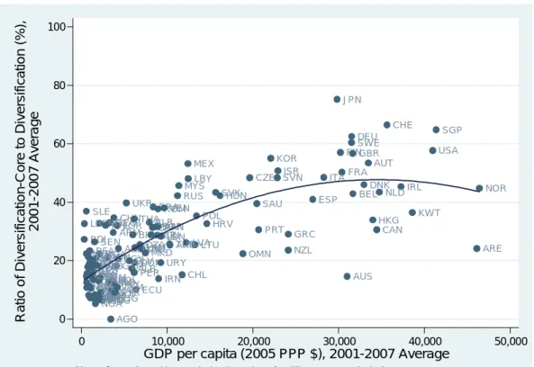
Figure 13 examines share-core across countries relative to their respective per capita income. As noted above, Mexico is a positive outlier, in the sense that it has a higher share of commodities in the core than would be expected for a country at its stage of development. Another point to be noted is that, while China and India were clear positive outliers in terms of diversification and diversification-core, they no longer stand out from the rest of countries in their income group when it comes to share-core (although they are above the fitted line, there are other countries in their income group also above the fitted line). Other non-high-income

countries that are significant positive outliers are Libya, Malaysia, and Russia.

In short, figures 12 and 13 show that high-income countries have, in general, a greater share of complex capabilities. For developing countries to reach the status of high-income countries, they will need to acquire more capabilities both by increasing the absolute number of core commodities in which they have a comparative advantage and by shifting the composition of products with comparative advantage towards core commodities.

Figure 13: Share-core and GDP Per Capita, Average 2001–07

AGO ALB ARE ARG ARM AUS AUT AZE BDI BEL BEN BFA BGD BGR BIH BLR BOL BRA CAF CAN CHE CHL CHN CIV CMRCOG COL CRI CZE DEU DNK DOM DZA ECU EGY ESP ETH FIN FRA GBR GEO GHA GIN GRC GTM HKG HND HRV HTI HUN IDN IND IRL IRN ISR ITA JAM JOR JPN KAZ KEN KGZ KHM KOR KWT LAO LBN LBR LBY LKA LTU LVA MAR MDA MDG MEX MKD MLI MNG MOZ MRT MWI MYS NER NGA NIC NLD NOR NPL NZL OMN PAK PAN PER PHL PNG POL PRT PRY ROM RUS RWA SAU SDN SEN SGP SLE SLV SVK SVN SWE SYR TCD TGO THA TJK TKM TUN TUR TZA UGA UKR URY USA UZB VEN VNMYEM ZAF ZMB 0 20 40 60 80 100 R a ti o o f D ive rsi fi c a ti o n -C o re t o D ive rsi fi c a ti o n (% ), 2 0 0 1 -2 00 7 A v era g e 0 10,000 20,000 30,000 40,000 50,000

(24)

22

5. STANDARDNESS

A complementary way of analyzing the export composition of a country is by examining how unique the export basket is. If a country exports product A with comparative advantage, how many other countries export the same product with comparative advantage, i.e., is the product exported by only a few countries or by many and therefore is a “standard” commodity? The

standardness of a country’s export is calculated as the average ubiquity of the commodities exported with comparative advantage by a country.10

A lower value of standardness indicates that the country’s export basket is more unique. Figure 14 shows the relationship between standardness and diversification. Even though by definition standardness and diversification are inversely related, the figure is informative because it shows that there are cases where two countries are diversified in a similar number of products, but their standardness differs. For example, Korea and Egypt export a similar number of products with comparative advantage, but Korea’s export package is more unique than Egypt’s.

10

Hidalgo and Hausmann (2009) compute standardness as follows:

∑

1 c _ic i c Standardness = ubiquity diversification (4)

where, diversification is the total number of commodities in which country c has a comparative advantage and

(25)

Figure 14: Standardness and Diversification, Average 2001–07 AGO ALB ARE ARG ARM AUS AUT AZE BDI BEL BEN BFA BGD BGR BIH BLR BOL BRA CAF CAN CHE CHL CHN CIV CMR COG COL CRI CZE DEU DNK DOM DZA ECU EGY ESP ETH FIN FRA GBR GEO GHA GIN GRC GTM HKG HND HRV HTI HUN IDN IND IRL IRN ISR ITA JAM JOR JPN KAZ KEN KGZ KHM KOR KWT LAO LBN

LBRLBY LKA LVALTU

MAR MDA MDG MEX MKD MLI MNG MOZ MRT MWI MYS NER NGA NIC NLD NOR NPL NZL OMN PAK PAN PER PHL PNG POL PRT PRY ROM RUS RWA SAU SDN SEN SGP SLE SLV SVK SVN SWE SYR TCD TGO THA TJK TKM TUN TUR TZA UGA UKR URY USA UZB VEN VNM YEM ZAF ZMB 10 20 30 40 50 S tan da rd n e s s , 2 0 0 1 -2 0 0 7 A v er a g e 0 50 100 150 200 250 300 350 Diversification, 2001-2007 Average

Note: Countries with population less than 2 million were excluded. Dashed lines correspond to the respective means of standardness and diversifcation.

The best positioned countries are those in the fourth quadrant (high diversification and more unique products), while the worst are in the second quadrant (low diversification and more standard products). Brazil, China, India, Poland, and Thailand are some of the non-high-income countries in the fourth quadrant. Russia and Malaysia, on the other hand, are on the border of the third and the fourth quadrants at a level of standardness similar to that of Brazil, China, and India. China and India are on far right and near to the bottom in the fourth quadrant, an area largely comprised of high-income countries.

Finally, figure 15 shows that given their per capita incomes, China and India have a highly unique export package, i.e., have a level of standardness below what one would expect for countries at their level of development. Other countries with a more unique export package than what would be expected given their level of income are Indonesia, Malaysia, Mexico, the Philippines, Thailand, and Vietnam.

(26)

24

Figure 15: Standardness and GDP Per Capita, Average 2001–07

AGO ALB ARE ARG ARM AUS AUT AZE BDI BEL BEN BFA BGD BGR BIH BLR BOL BRA CAF CAN CHE CHL CHN CIV CMR COG COL CRI CZE DEU DNK DOM DZA ECU EGY ESP ETH FIN FRA GBR GEO GHA GIN GRC GTM HKG HND HRV HTI HUN IDN IND IRL IRN ISR ITA JAM JOR JPN KAZ KEN KGZ KHM KOR KWT LAO LBN

LBR LKA LVALBYLTU

MAR MDA MDG MEX MKD MLI MNG MOZ MRT MWI MYS NER NGA NIC NLD NOR NPL NZL OMN PAK PAN PER PHL PNG POL PRT PRY ROM RUS RWA SAU SDN SEN SGP SLE SLV SVK SVN SWE SYR TCD TGO THA TJK _TKM TUN TUR TZA UGA UKR URY USA UZB VEN VNM YEM ZAF ZMB 10 20 30 40 50 S tan da rd n e s s , 2 0 0 1 -2 0 0 7 A v er a g e 6 7 8 9 10 11 12

GDP per capita (2005 PPP $, in logs), 2001-2007 Average

6. OPEN FOREST

The discussion so far has focused on the composition of the current export basket. In this section we ask how far the products currently not exported with comparative advantage are from this basket. In other words, given the current capability set, what is the likelihood of exporting these other products with comparative advantage? This measure, called “open forest” (Hausmann and Klinger 2006), is the last factor that enters our Index of Opportunities.

Open forest provides a measure of the (expected) value of the goods that a country could potentially export, i.e., the products that it currently does not export with comparative advantage. This value depends on how far the non-exported goods are from the goods currently being exported with comparative advantage, and on the sophistication level of these non-exported goods. It is calculated as the weighted average of the sophistication level of all potential exports of a country (i.e., those goods not yet exported with comparative advantage), where the weight is

(27)

the density or distance between each of these goods and those exported with comparative advantage (see section 2 for the definition of density).11

One may conclude that, because the developed countries, in general, export more products with comparative advantage than the developing countries, the possibilities for further diversification of the developed countries (and, therefore, of a high value of open forest) are limited. However, this is not exactly what matters for the purposes of open forest. Developed countries have comparative advantage in sophisticated products (e.g., some types of machinery). These products are “close” to many other sophisticated products, for example, other types of machinery or chemicals, in the sense that there is a high probability that the country can export them successfully (i.e., that it can acquire comparative advantage) because these products use capabilities similar to the ones the country already possesses. On the other hand, there are products that are “far” from the current basket (i.e., greater distance and hence low probability that the country acquires comparative advantage in them) and developed countries will probably not export them. These products tend to have low sophistication (e.g., natural resources, some agricultural products) and contribute little to open forest. Therefore, even though developed countries have revealed comparative advantage in the export of a large number of goods, many of the products that they do not export with comparative advantage are highly sophisticated and the probability of exporting them is high. Hence the relatively high open forest of these

countries.

The opposite is true for developing countries. Even though they can potentially export many products (those in which they do not have a comparative advantage) and most of them are

11 Algebraically: ω ⎡ ⎤ =

∑

_⎣ − _⎦ _ _c _cj(1 _cj) _j j

Open Forest x PRODY (5)

where φ ω φ =

∑

ij ci i cj ij i x is the density; ≥ ⎧⎪ = ⎨ _< ⎪⎩ , ,

1 if RCA 1 for country

,

0 if RCA 1 for country

i j ci cj

i j

c x x

c;ϕij denotes the proximity

or probability that the country will shift resources into good j (not exported with comparative advantage), given that it exports good i; PRODYj (see equation 1) is a measure of the sophistication of product j (not exported with comparative advantage); and ωcjPRODYj is the expected value (in terms of the sophistication of exports) of good j. Open forest is measured in 2005 PPP$.

(28)

26

sophisticated (e.g., machinery), the probability that these countries export them is low because they do not have the capabilities to do it (i.e., they are from the current export basket). Hence the low open forest of these economies.

Figure 16 shows the value of open forest of various countries. For the reasons discussed above, high-income countries have a very high value of open forest: the goods not exported with comparative advantage that are close to their current export basket are highly sophisticated. Among the developing countries, Poland has the highest open forest ($2,602,986), followed by India ($2,284,511), Turkey ($2,268,770), and China ($2,227,843). Other than China and India, no other lower-middle-income country has such a high open forest. Other countries with high open forest values are Ukraine ($1,940,032), Thailand ($1,928,222), Indonesia ($1,898,851), and Brazil ($1,978,485). Russia ($1,185,006) has a significantly lower open forest, whichhighlights the lower opportunities for further diversification available given the sophistication level of their current export basket.

Figure 16: Open Forest, Average 2001–07

0 500 1,000 1,500 2,000 2,500 3,000 Uruguay Pakistan Kenya Bosnia Malaysia Russia Panama Guatemala Lebanon Viet Nam Jordan Tunisia Egypt Colombia Argentina Belarus Latvia Mexico Lithuania Indonesia Romania Thailand Ukraine Brazil Bulgaria South Africa China Turkey India Poland

0 500 1,000 1,500 2,000 2,500 3,000 Ireland Norway Singapore Australia New Zealand Israel Hong Kong Rep. of Korea Finland Croatia Japan Greece Canada Switzerland Hungary Portugal Slovakia Sweden Slovenia Denmark Netherlands UK Germany USA Austria Czech Rep. Belgium Italy France Spain

Open Forest ('000, 2005 PPP $), 2001-2007 Average

(29)

Figure 17 shows the regression of open forest and per capita income. Given their stage of development, China and India are clear outliers in that their open forest is much higher than what is predicted by the regression. Other countries that have similar open forest values to China and India are Poland and Turkey. However, they have higher per capita income.

Figure 17: Open Forest and GDPpc, Average 2001–07

AGO ALB ARE ARG ARM AUS AUT AZE BDI BEL BEN BFA BGD BGR BIH BLR BOL BRA CAF CANCHE CHL CHN CIV CMR COG COL CRI CZE DEU DNK DOM DZA ECU EGY ESP ETH FIN FRA GBR GEO GHA GIN GRC GTM HKG HND HRV HTI HUN IDN IND IRL IRN ISR ITA JAM JOR JPN KAZ KEN KGZ KHM KOR KWT LAO LBN LBR LBY LKA LTU LVA MAR MDA MDG MEX MKD MLIMNG MOZ MRT MWI MYS NER NGA NIC NLD NOR NPL NZL OMN PAK PAN PER PHL PNG POL PRT PRY ROM RUS RWA SAU SDN SEN SGP SLE SLV SVK SVN SWE SYR TCD TGO THA TJK _TKM TUN TUR TZA UGA UKR URY USA UZB VEN VNM YEM ZAF ZMB 0 500 1,000 1,500 2,000 2,500 3,000 O p e n F o re st ('0 0 0 , 2 0 0 5 PPP $ ), 2 0 0 1 -2 00 7 A v era g e 0 10,000 20,000 30,000 40,000 50,000

7. AS YOU SOW, SO SHALL YOU REAP: INDEX OF OPPORTUNITIES

We have used the product space to infer countries’ capabilities and the opportunities they

provide for further structural change. The existing capabilities of a country are an indicator of its capacity to transform its portfolio of exports from less sophisticated products to more

sophisticated products, and thereby generate future growth. In previous sections, capabilities have been summarized in the form of seven indicators, namely, EXPY (figure 2), EXPY-core (figure 6), diversification (figure 8), diversification-core (figure 10), share-core (figure 12),

(30)

28

standardness (figure 14), and open forest (figure 16). In the previous sections we have shown the top thirty countries according to each indicator. Based on these charts, some countries

consistently appear in the top thirty, while others are in the top thirty only in some of the indicators. On the other hand, if we look at the performance of some countries relative to their per capita incomes (figures 5, 7, 9, 11, 13, 15, and 17), we see that some countries are better off than what would be expected. In this aspect, China and India stand out.

In this section, we combine the information discussed previously and develop a new Index of Opportunities to rank countries on the basis of their accumulated capabilities. We present two indices. The first one ranks only developing countries (a total of 96 countries), while the second one includes developed countries (a total of 130 countries). Our methodology is designed to “reward” countries that perform well given their income per capita and “penalize” those that perform poorly given their income per capita. We do this as follows.

We estimate cross-country regressions (using data for both high-income and non-high-income countries) of each of the seven indicators on the level of GDP per capita. 12 Each

indicator has two components that enter the construction of the index. One is the actual value of the indicator, which captures the actual capabilities. The other one is the residual from the regression of the indicator on GDP per capita. This shows whether a country is a positive or a negative outlier given its current stage of development. The residual obtained in each case is considered a “reward” or a “penalty.” For example, consider export sophistication. The

procedure we use involves running a regression of our measure of export sophistication (EXPY) on GDP per capita (where both are specified in levels). The residual obtained from this

regression is a reward if it is positive and a penalty if the residual is negative. This procedure is repeated for the other six indicators. Referring back to our discussion of standardness in section 5, a lower value is considered better. In this case, therefore, a negative residual corresponds to a reward and a positive residual to a penalty.

These seven indicators and their residuals from the regressions on GDP per capita are, however, not comparable directly because they have different units. To solve this problem, we rescale all seven indicators and the residuals such that they lie between 0 (minimum value) and 1

12

We use the average for the period 2001–07 for each of the seven indicators and for GDP per capita. For

diversification, diversification-core, share-core, and open forest, the square of GDP per capita was also included as regressor (see figures 9, 11, 13, and 17)

(31)

(maximum value).13 For purposes of the construction and rescaling of the first index, we do not include the high-income countries, since we are interested only in the future opportunities for further transformation of the non-high-income countries. An increasing value, except in the case of standardness, is considered better. To average across the seven indicators we need to ensure that an increasing value of standardness (and its residual) also corresponds to an improvement. We do so by subtracting the rescaled value of standardness from 1. With all the seven indicators (and their residuals) scaled to lie between 0 and 1, and an increasing value corresponding to an improvement, we averaged the fourteen components to obtain the Index of Opportunities.

Table 1 shows the seven indicators (and their corresponding residuals) and the Index of Opportunities for the 96 non-high-income countries. A higher value of the index indicates that a country has accumulated more capabilities, and this provides the country with more

opportunities to generate and sustain further transformation and growth. 14

Table 1 shows that, among the non-high-income countries, China has the highest score, followed by India, Poland, Thailand, and Mexico. Brazil comes in 6th place and Russia in 18th. Other Asian countries well placed are Indonesia (8th), Malaysia (10th), the Philippines (13th), Vietnam (21st), and Georgia (29th). China and Thailand rank in the first quintile in all indicators. On the other hand, some Asian countries are ranked in the fourth and fifth quintiles (Tajikistan, Bangladesh, Turkmenistan, Lao PDR, Mongolia, and Cambodia). This low ranking is a

reflection of these countries’ export baskets’ position in the product space (in general, low diversification and sophistication). Obviously, this can be reversed through policies to, for example, help develop new capabilities.

So far we have discussed the growth opportunities of non-high-income countries. Table 2 shows the Index of Opportunities for both the high-income and the non-high-income countries (130 countries). To construct this index, we repeat the exercise described previously and rescale each of the indicators (to lie between 0 and 1), this time also including the high-income

countries.15

13

Each indicator is rescaled as follows. Suppose the original value of the indicator i is X, and the rescaled value is

Xnew. Then, Xnew =(X- Xmin)/( Xmax - Xmin) where, Xmin (Xmax) is the minimum (maximum) value of indicator i among

the set of non-high-income countries in table 1.

14

We have also checked if the ranking is influenced by the choice of period over which the data is averaged. We constructed the Index of Opportunities based on averages for 2003–07 and 2005–07, and find that the respective correlations with the reported index for 2001–07 are very high: 0.995 and 0.987, respectively.

15

(32)

30

As expected, the high-income countries dominate the top twenty. However, what is interesting is that the top eight countries in table 1 (except Ukraine) make it to the top twenty in table 2: China is third behind Germany and the United States; India is fifth, just behind Japan, and ahead of France and Italy; Poland is ranked 14th; Thailand is ranked 15th; Brazil 18th; Mexico 19th; and Indonesia 20th. Not only do these seven countries rank very high in terms of the overall score, but also rank high on most individual indicators.16

While most of the high income countries are in the top quintile, there are a few that lie in the fifth quintile. These are commodity-rich countries such as Saudi Arabia, Oman, UAE, and Kuwait. These countries do not perform well on any of the components, especially with respect to the diversification of their exports baskets, their low presence in the core, and their low future opportunities.

16

Some of the 14 components are highly correlated with each other. Out of the 91 possible correlations, 18 are greater than 0.7 (in the sample of all countries). One may argue then that these variables are capturing similar information. To avoid this problem, we constructed the index using the first component obtained from a principal components analysis (PCA). The first principal component accounts for 51.3% of the total variance of the variables. The Pearson correlation between the index shown here and that obtained from the PCA is 0.99 and the rank

correlation between the two is 0.99. Given this, we decided to continue working with the index based on the 14 variables.

(33)

Table 1: Index of Opportunities and its Components: Non-high-income Countries

COLOR LEGEND FIRST QUINTILE 2nd QUINTILE 3rd QUINTILE 4th QUINTILE FIFTH QUINTILE

EXPY EXPY-Core Diversification

Diversification-Core Share Core Standardness Open Forest

Country

Actual Residual Actual Residual Actual Residual Actual Residual Actual Residual Actual Residual Actual Residual

Index of Opportunities Rank China 0.8921 0.9020 0.8694 0.9006 0.9698 0.9767 0.9496 0.9918 0.6497 0.8077 0.9352 1.0000 0.8538 0.9174 0.9011 1 India 0.6486 0.6746 0.9328 0.9874 0.9287 1.0000 0.8611 1.0000 0.6148 0.8399 0.7917 0.8698 0.8759 1.0000 0.8590 2 Poland 0.9105 0.7054 0.8170 0.7393 1.0000 0.7581 1.0000 0.6840 0.6642 0.4721 0.7070 0.5694 1.0000 0.7611 0.7706 3 Thailand 0.8703 0.8254 0.8647 0.8700 0.7411 0.7202 0.7221 0.7186 0.6450 0.7035 0.7656 0.7672 0.7370 0.7410 0.7637 4 Mexico 0.9689 0.7919 0.8746 0.8123 0.5436 0.4081 0.8290 0.5819 1.0000 0.9297 0.8260 0.7213 0.6549 0.5014 0.7460 5 Brazil 0.7127 0.6036 0.8105 0.7874 0.7142 0.6382 0.7802 0.6787 0.7208 0.7137 0.8795 0.8548 0.7566 0.6885 0.7385 6 Ukraine 0.7136 0.6751 0.5542 0.5458 0.6862 0.7027 0.7771 0.7981 0.7467 0.8700 0.7208 0.7335 0.7416 0.7753 0.7172 7 Indonesia 0.7564 0.7702 0.8256 0.8613 0.8042 0.8661 0.4840 0.6647 0.3982 0.5204 0.6976 0.7465 0.7255 0.8396 0.7114 8 South Africa 0.6911 0.5821 0.7677 0.7424 0.7811 0.6947 0.6962 0.6172 0.5892 0.5500 0.7067 0.6626 0.7960 0.7233 0.6857 9 Malaysia 1.0000 0.8501 0.8791 0.8289 0.3977 0.3122 0.5252 0.3808 0.8592 0.7854 1.0000 0.9361 0.4427 0.3533 0.6822 10 Romania 0.6744 0.5491 0.6960 0.6581 0.7301 0.6369 0.7832 0.6608 0.7072 0.6758 0.6647 0.6036 0.7278 0.6490 0.6726 11 Bulgaria 0.6825 0.5622 0.7418 0.7094 0.8042 0.7015 0.7237 0.6215 0.5951 0.5402 0.5945 0.5282 0.7656 0.6850 0.6611 12 Philippines 0.9618 1.0000 0.8399 0.8794 0.3719 0.5247 0.3466 0.5701 0.6028 0.7916 0.6513 0.6992 0.3782 0.5659 0.6560 13 Belarus 0.8946 0.8122 0.7152 0.6898 0.5612 0.5260 0.5328 0.5045 0.6193 0.6017 0.7032 0.6652 0.6389 0.6058 0.6479 14 Turkey 0.6906 0.5359 0.7186 0.6675 0.8859 0.7303 0.6443 0.5064 0.4818 0.3411 0.6134 0.5211 0.8697 0.7277 0.6382 15 Argentina 0.6398 0.4794 0.8959 0.8577 0.6018 0.4992 0.4366 0.3447 0.4762 0.3323 0.6964 0.6134 0.6180 0.5210 0.5723 16 Jordan 0.6064 0.5818 0.6653 0.6767 0.4707 0.5606 0.4336 0.5776 0.5999 0.7282 0.4763 0.4783 0.5092 0.6226 0.5705 17 Russian Federation 0.7445 0.5743 0.5901 0.5192 0.3856 0.3052 0.4718 0.3437 0.7910 0.7031 0.9050 0.8318 0.4473 0.3602 0.5695 18 Egypt 0.7451 0.7309 0.6459 0.6548 0.5771 0.6437 0.3405 0.5016 0.3860 0.4524 0.4595 0.4576 0.5605 0.6610 0.5583 19 Latvia 0.7532 0.5607 0.7520 0.6823 0.6698 0.5138 0.4992 0.3330 0.4855 0.2820 0.5455 0.4099 0.6421 0.4950 0.5446 20 Viet Nam 0.5168 0.5329 0.7512 0.7929 0.5584 0.7034 0.2122 0.5037 0.2480 0.3783 0.5695 0.6221 0.5047 0.7006 0.5425 21 Bosnia Herzegovina 0.6099 0.5451 0.7370 0.7343 0.4997 0.5296 0.4137 0.4873 0.5384 0.5746 0.4735 0.4425 0.4414 0.5052 0.5380 22 Lithuania 0.7530 0.5375 0.6579 0.5699 0.7197 0.5344 0.5206 0.3194 0.4734 0.2352 0.5352 0.3798 0.7095 0.5278 0.5338 23 Sierra Leone 0.4226 0.4622 0.8363 0.9001 0.1711 0.4408 0.1924 0.5563 0.6845 1.0000 0.5737 0.6527 0.1229 0.4472 0.5331 24 Colombia 0.6311 0.5437 0.7434 0.7294 0.5030 0.5016 0.3466 0.3927 0.4505 0.4198 0.4990 0.4513 0.5609 0.5677 0.5243 25 Lebanon 0.6465 0.5112 0.6140 0.5662 0.5869 0.5128 0.4733 0.4100 0.5250 0.4323 0.5448 0.4630 0.4984 0.4524 0.5169 26 Uruguay 0.6930 0.5626 1.0000 0.9820 0.4531 0.4052 0.2519 0.2404 0.3617 0.2261 0.6255 0.5541 0.4187 0.3883 0.5116 27 Panama 0.6389 0.5097 0.5503 0.5008 0.4761 0.4305 0.4336 0.3900 0.5941 0.5310 0.6050 0.5360 0.4531 0.4238 0.5052 28 Georgia 0.5411 0.5308 0.6291 0.6476 0.2825 0.4373 0.2748 0.4945 0.6208 0.7941 0.5345 0.5599 0.2612 0.4532 0.5044 29

(34)

32

EXPY EXPY-Core Diversification Diversification-_Core Share Core Standardness Open Forest

Country

Index of Opportunities Rank Costa Rica 0.7682 0.6530 0.8434 0.8175 0.3313 0.3158 0.2779 0.2736 0.5386 0.4643 0.4241 0.3349 0.3677 0.3571 0.4834 31 Kenya 0.3312 0.3460 0.6703 0.7134 0.4783 0.6630 0.2382 0.5565 0.3255 0.5091 0.3881 0.4312 0.4383 0.6744 0.4831 32 Nepal 0.4112 0.4421 0.5926 0.6340 0.4032 0.6161 0.2214 0.5621 0.3569 0.5675 0.5219 0.5884 0.2041 0.4992 0.4729 33 Kyrgyzstan 0.3315 0.3381 0.7038 0.7455 0.3939 0.5817 0.2366 0.5381 0.3954 0.5809 0.4868 0.5353 0.2384 0.4966 0.4716 34 Rep. of Moldova 0.4881 0.5008 0.4516 0.4700 0.4010 0.5749 0.2565 0.5365 0.4137 0.5873 0.4211 0.4551 0.3094 0.5401 0.4576 35 Venezuela 0.7488 0.6142 0.7138 0.6694 0.1843 0.1777 0.2122 0.1955 0.7128 0.6573 0.5759 0.4909 0.2159 0.2116 0.4557 36 Pakistan 0.3447 0.3434 0.8006 0.8453 0.4800 0.6374 0.1053 0.4180 0.1421 0.2404 0.4485 0.4850 0.4379 0.6434 0.4551 37 Armenia 0.4695 0.4425 0.5886 0.5991 0.2545 0.4001 0.2229 0.4347 0.5438 0.6766 0.5339 0.5511 0.2036 0.3896 0.4507 38 Guatemala 0.3683 0.3245 0.7188 0.7356 0.4882 0.5785 0.2550 0.4448 0.3423 0.4061 0.2868 0.2677 0.4554 0.5829 0.4468 39 Syria 0.6003 0.5815 0.8088 0.8343 0.3955 0.5089 0.1038 0.3356 0.1487 0.1676 0.4612 0.4665 0.3399 0.4948 0.4462 40 Senegal 0.4249 0.4433 0.3272 0.3416 0.3703 0.5677 0.2840 0.5814 0.4889 0.7064 0.3726 0.4098 0.3126 0.5629 0.4424 41 Azerbaijan 0.7036 0.6844 0.7837 0.8026 0.1635 0.3072 0.1206 0.3297 0.4524 0.5344 0.4125 0.4039 0.1523 0.3260 0.4412 42 Kazakhstan 0.6288 0.5182 0.4090 0.3583 0.2946 0.3056 0.2489 0.2790 0.5435 0.4989 0.7462 0.7102 0.2843 0.3112 0.4383 43 Sri Lanka 0.3259 0.2930 0.8535 0.8878 0.4279 0.5506 0.1023 0.3555 0.1546 0.1962 0.4957 0.5139 0.3657 0.5336 0.4326 44 El Salvador 0.5639 0.5034 0.7947 0.8006 0.3631 0.4302 0.2107 0.3462 0.3758 0.3839 0.2610 0.2110 0.3491 0.4426 0.4312 45 Uzbekistan 0.3078 0.3072 0.6818 0.7194 0.2512 0.4584 0.1359 0.4499 0.3420 0.5026 0.5251 0.5742 0.2071 0.4621 0.4232 46 Peru 0.3945 0.3063 0.6492 0.6380 0.4432 0.4791 0.2031 0.3182 0.2983 0.2632 0.4984 0.4674 0.4070 0.4717 0.4170 47 TFYR of Macedonia 0.5379 0.4333 0.4939 0.4566 0.4745 0.4680 0.3099 0.3497 0.4255 0.3731 0.3847 0.3160 0.3763 0.4053 0.4146 48 Burundi 0.1526 0.1735 0.8410 0.9080 0.0944 0.3882 0.0840 0.4855 0.4478 0.7121 0.4901 0.5636 0.0152 0.3703 0.4090 49 Dominican Rep. 0.5426 0.4665 0.6477 0.6358 0.3769 0.4236 0.2107 0.3217 0.3602 0.3393 0.3082 0.2529 0.3488 0.4222 0.4041 50 Ethiopia 0.0998 0.1100 0.9063 0.9753 0.2628 0.5148 0.1145 0.4962 0.2251 0.4165 0.3999 0.4577 0.1797 0.4934 0.4037 51 Mozambique 0.4359 0.4758 0.7430 0.7991 0.1766 0.4437 0.0672 0.4578 0.2299 0.4208 0.3578 0.4097 0.1271 0.4489 0.3995 52 Libya 0.7513 0.5535 0.7880 0.7186 0.0406 0.0000 0.0763 0.0000 0.9045 0.8069 0.5167 0.3735 0.0417 0.0000 0.3980 53 Uganda 0.2108 0.2248 0.6894 0.7388 0.2891 0.5259 0.1481 0.5085 0.3152 0.5175 0.3112 0.3531 0.1903 0.4904 0.3938 54 Algeria 0.9577 0.9057 0.6144 0.5932 0.0483 0.1405 0.0458 0.1707 0.4678 0.4518 0.4778 0.4322 0.0447 0.1546 0.3932 55 Iran 0.7199 0.5966 0.7583 0.7241 0.2222 0.2234 0.0916 0.1241 0.2547 0.0979 0.6408 0.5751 0.2318 0.2416 0.3930 56 Togo 0.2559 0.2765 0.5504 0.5904 0.2902 0.5309 0.1832 0.5410 0.3939 0.6229 0.2650 0.3032 0.1656 0.4749 0.3889 57 Bolivia 0.3884 0.3577 0.7216 0.7440 0.2688 0.4168 0.1053 0.3510 0.2501 0.3107 0.4673 0.4793 0.1929 0.3868 0.3886 58 Yemen 0.6997 0.7298 0.7323 0.7713 0.1465 0.3659 0.0641 0.3842 0.2358 0.3574 0.2149 0.2221 0.1268 0.3878 0.3885 59

United Rep. of Tanzania 0.1865 0.1957 0.6193 0.6622 0.3873 0.6015 0.1252 0.4856 0.2015 0.3678 0.3518 0.3966 0.2612 0.5438 0.3847 60

Albania 0.4280 0.3489 0.6994 0.6949 0.4054 0.4563 0.2031 0.3291 0.3265 0.3100 0.3116 0.2626 0.2494 0.3520 0.3841 61

Chad 0.3500 0.3686 0.8342 0.8908 0.0181 0.2938 0.0183 0.3914 0.3098 0.4937 0.4887 0.5458 0.0000 0.3206 0.3803 62

Chile 0.5128 0.3098 0.7205 0.6540 0.3993 0.3053 0.1756 0.0990 0.2849 0.0435 0.5639 0.4398 0.4114 0.3185 0.3742 63

Mali 0.0765 0.0761 0.6961 0.7450 0.1399 0.4017 0.0901 0.4592 0.3901 0.6081 0.4646 0.5235 0.1121 0.4228 0.3718 64

(35)

EXPY EXPY-Core Diversification Diversification-_Core Share Core Standardness Open Forest Country

Index of Opportunities Rank Morocco 0.4378 0.4133 0.3764 0.3732 0.4229 0.5439 0.1191 0.3649 0.1826 0.2282 0.3582 0.3582 0.3803 0.5425 0.3644 66 Burkina Faso 0.0134 0.0070 0.6993 0.7483 0.2024 0.4519 0.1420 0.4986 0.3872 0.6038 0.3637 0.4100 0.1198 0.4285 0.3626 67 Nigeria 0.7644 0.8116 0.5961 0.6301 0.0664 0.3185 0.0122 0.3675 0.0972 0.2047 0.3800 0.4165 0.0529 0.3473 0.3618 68 Ghana 0.1916 0.1976 0.7093 0.7572 0.2463 0.4814 0.0763 0.4400 0.1910 0.3467 0.3494 0.3910 0.1986 0.4859 0.3616 69 Tajikistan 0.3036 0.3149 0.7657 0.8155 0.1459 0.3924 0.0611 0.4179 0.2525 0.4145 0.3310 0.3663 0.0824 0.3822 0.3604 70 Ecuador 0.4911 0.4066 0.8610 0.8635 0.2573 0.3222 0.0763 0.2116 0.1866 0.1123 0.3692 0.3184 0.2358 0.3248 0.3598 71 Paraguay 0.3051 0.2600 0.6309 0.6432 0.2633 0.4026 0.0931 0.3284 0.2236 0.2639 0.5100 0.5217 0.1915 0.3746 0.3580 72 Bangladesh 0.2768 0.2935 0.7820 0.8369 0.2386 0.4798 0.0519 0.4273 0.1387 0.2864 0.2348 0.2647 0.2010 0.4932 0.3576 73 Côte d’Ivoire 0.1877 0.1838 0.3360 0.3508 0.2545 0.4730 0.1420 0.4705 0.3531 0.5325 0.4264 0.4697 0.2256 0.4908 0.3497 74 Madagascar 0.2384 0.2551 0.7061 0.7569 0.3017 0.5365 0.0718 0.4501 0.1500 0.3081 0.1903 0.2176 0.1929 0.4930 0.3477 75 Sudan 0.6004 0.6343 0.7060 0.7492 0.1163 0.3614 0.0305 0.3850 0.1542 0.2803 0.1826 0.1962 0.0886 0.3793 0.3475 76 Angola 0.6932 0.6938 0.9578 1.0000 0.0000 0.2043 0.0000 0.2767 0.0000 0.0000 0.3913 0.3968 0.0019 0.2368 0.3466 77 Rwanda 0.1347 0.1443 0.7042 0.7560 0.0790 0.3602 0.0473 0.4365 0.3104 0.5170 0.4357 0.4949 0.0329 0.3669 0.3443 78 Congo 0.6124 0.6064 0.8430 0.8768 0.0762 0.2670 0.0183 0.2922 0.1312 0.1680 0.2854 0.2786 0.0517 0.2786 0.3419 79 Turkmenistan 0.5389 0.5087 0.6915 0.7053 0.0949 0.2573 0.0336 0.2702 0.2019 0.2239 0.3466 0.3332 0.0643 0.2605 0.3236 80

Central African Rep. 0.1176 0.1280 0.7453 0.8014 0.0433 0.3350 0.0260 0.4250 0.2714 0.4724 0.3618 0.4138 0.0190 0.3599 0.3229 81

Honduras 0.2913 0.2604 0.3653 0.3647 0.3379 0.4853 0.1237 0.3822 0.2355 0.3092 0.3044 0.3035 0.2778 0.4704 0.3222 82

Lao People’s Dem. Rep. 0.2302 0.2296 0.7534 0.7999 0.2134 0.4389 0.0504 0.3987 0.1443 0.2662 0.1919 0.2061 0.0928 0.3814 0.3141 83

Papua New Guinea 0.2421 0.2363 0.7431 0.7857 0.1295 0.3611 0.0260 0.3668 0.1214 0.2242 0.3265 0.3521 0.0903 0.3682 0.3124 84

Niger 0.2172 0.2386 0.0000 0.0000 0.1607 0.4331 0.1099 0.4938 0.4197 0.6647 0.4860 0.5548 0.1180 0.4441 0.3101 85 Mongolia 0.1921 0.1683 0.7257 0.7604 0.2150 0.4098 0.0412 0.3510 0.1197 0.1945 0.3251 0.3397 0.1177 0.3671 0.3091 86 Cameroon 0.3713 0.3761 0.6908 0.7288 0.1245 0.3553 0.0305 0.3678 0.1412 0.2467 0.1684 0.1737 0.1048 0.3780 0.3041 87 Zambia 0.2565 0.2698 0.1582 0.1646 0.1942 0.4414 0.0870 0.4511 0.2798 0.4623 0.4158 0.4666 0.1538 0.4519 0.3038 88 Nicaragua 0.2838 0.2736 0.4968 0.5166 0.2918 0.4800 0.0779 0.3899 0.1686 0.2672 0.1317 0.1268 0.2062 0.4484 0.2971 89 Jamaica 0.3380 0.2272 0.4139 0.3763 0.1821 0.2459 0.1359 0.2360 0.4618 0.4400 0.2725 0.1999 0.1879 0.2681 0.2847 90 Cambodia 0.2709 0.2801 0.5499 0.5837 0.1843 0.4248 0.0397 0.4032 0.1320 0.2633 0.1407 0.1535 0.1277 0.4208 0.2839 91 Guinea 0.2350 0.2477 0.6868 0.7343 0.0976 0.3655 0.0336 0.4129 0.1955 0.3583 0.0740 0.0842 0.0614 0.3791 0.2833 92 Malawi 0.0000 0.0000 0.6942 0.7466 0.1585 0.4288 0.0519 0.4457 0.1948 0.3758 0.1485 0.1748 0.0877 0.4164 0.2803 93 Benin 0.1257 0.1223 0.5008 0.5312 0.1448 0.3938 0.0687 0.4269 0.2792 0.4515 0.2069 0.2284 0.0684 0.3735 0.2802 94 Mauritania 0.3423 0.3505 0.7956 0.8446 0.0521 0.3059 0.0122 0.3661 0.1157 0.2268 0.0721 0.0705 0.0272 0.3252 0.2791 95 Haiti 0.2620 0.2758 0.2587 0.2729 0.1487 0.4046 0.0504 0.4229 0.2092 0.3726 0.0000 0.0000 0.0666 0.3807 0.2232 96