SPATIAL AND TEMPORAL PATTERNS OF GASTROINTESTINAL ILLNESS AND THEIR RELATIONSHIP WITH PRECIPITATION ACROSS THE STATE OF NORTH CAROLINA
JENNA M. HARTLEY
A thesis submitted to the faculty at the University of North Carolina at Chapel Hill in partial fulfillment of the requirements for the degree of Master of Science in the Department of Environmental Sciences and Engineering in the Gillings School of Global Public Health.
Chapel Hill 2016
Approved by: J. Jason West Charles E. Konrad
ABSTRACT
Jenna M. Hartley: Spatial and temporal patterns of gastrointestinal illness and their relationship with precipitation across the state of North Carolina
(Under the direction of J. Jason West and Charles E. Konrad)
The quality of drinking water quality in the United States is among the best in the world. Nonetheless, pathogens are present in source waters that are used for drinking water. Water in general and floodwaters specifically can spread pathogens within watersheds by mobilizing pathogens in the environment and transporting them. Previous research has identified a positive association between gastrointestinal illness and meteorological variables, including heavy
precipitation. This study analyzes patterns of gastrointestinal illness and their relationship with various demographic variables and precipitation across the state of North Carolina. Results show the strongest demographic relationships between poverty indicators and disease. Moreover, this study identifies increases in the rate of gastrointestinal illness after periods of heavy rainfall. Several geographical clusters of high disease occurrence are identified at the county level, with seven
ACKNOWLEDGEMENTS
This project was developed with assistance and support of the Southeast Regional Climate Center (SERCC), the North Carolina State Climate Office, and the Carolinas Integrated Science Assessments (CISA). The Emergency Department health data was made available by the North Carolina Disease Event Tracking and Epidemiologic Collection Tool (NC DETECT). NC DETECT is North Carolina’s statewide syndromic surveillance system, which is funded by the North Carolina Division of Public Health (NC DPH) Federal Public Health Emergency
Preparedness Grant and managed through a collaboration between NC DPH and the University of North Carolina at Chapel Hill’s Department of Emergency Medicine’s Carolina Center for Health Informatics. The NC DETECT oversight committee does not take responsibility for the scientific validity or accuracy of methodology, results, statistical analyses, or conclusions presented in this project.
Special thanks to Ashley Hiatt with the North Carolina State Climate Office for assisting with the extraction of the climate and health data, Margaret (Maggie) Sugg with Appalachian State University (formerly with SERCC) for her kind mentorship and guidance, Jordan McLeod and William Schmitz with SERCC for their assistance with ArcGIS tools and precipitation interpretation, respectively, and to Kristen Downs with the University of North Carolina at Chapel Hill
Environmental Sciences and Engineering Department for her assistance with planning and thought-process development throughout the development of the project.
TABLE OF CONTENTS
LIST OF TABLES………. viii
LIST OF FIGURES………... ix
LIST OF ABBREVIATIONS………... xi
CHAPTER 1: ACUTE GASTROINTESTINAL ILLNESS AND DIARRHEA…………... 1
Introduction: Gastrointestinal Disease and Diarrhea………... 1
Disease Burden………...……….... 3
Pathways to Human Exposure: Overview……….. 3
Pathways to Human Exposure: The impact of heavy rains on drinking water and recreational water contamination……….. 5
Links between precipitation and gastrointestinal illness, AGI, and diarrhea……….... 8
Connection to Climate Change………... 11
Overall Objectives of this Study………... 13
CHAPTER 2: METHODS……….. 15
Data Sources and IRB Exemption………... 15
Health Data………... 15
Demographic Data………... 19
Meteorological Data………... 21
Geographic Data……….... 27
Mapping of Spatial Patterns……….... 28
CHAPTER 3: RESULTS………. 31
Introduction……… 31
Descriptions of temporal patterns……….………...…... 31
Spatial patterns……….………... 34
Demographic patterns……… 42
Precipitation patterns..………... 52
CHAPTER 4: DISCUSSION………... 59
Study Limitations……… 60
Future Research………... 62 APPENDIX 3.1: ANNUAL VARIATION MAPS, NATURAL BREAKS………. APPENDIX 3.2: ANNUAL VARIATION MAPS, QUANTILES……….. APPENDIX 3.3: AGE GROUP MAPS, ALL AGE GROUPS….………... APPENDIX 3.4: AGE GROUP MAPS, SPECIFIC AGE GROUPS…...……… REFERENCES………...
LIST OF TABLES
Table 1 – ICD-9-CM codes utilized in study………... 18
Table 2 – Definitions of “heavy precipitation” for this study……….. 25
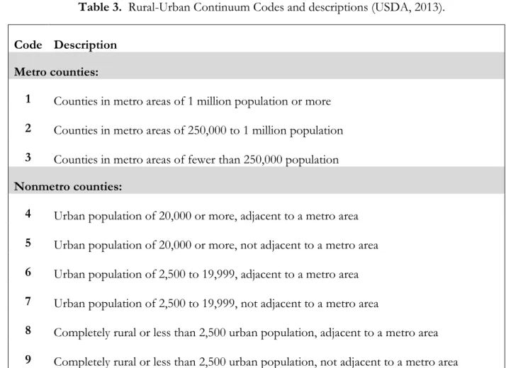
Table 3 – Rural-Urban Continuum Codes and their descriptions……… 28
Table 4 – Correlation Matrix: Rates & Demographic Variables………... 51
LIST OF FIGURES
Figure 1 – Diagram of Combined Sewer Systems………. 6
Figure 2 – Locations of United States communities served by Combined Sewer Systems……. 7
Figure 3 – Map of all North Carolina Emergency Departments that report to NC DETECT……….... 17
Figure 4 – Features of the NC DETECT Climate-Health Toolbox ………. 23
Figure 5 – Total Counts of gastrointestinal illness, separated by time of day………. 32
Figure 6 – Total Counts of gastrointestinal illness, separated by month of year……… 33
Figure 7 – Total Counts of gastrointestinal illness, separated by day of year ……… 33
Figure 8 –North Carolina county level gastrointestinal illness map………... 34
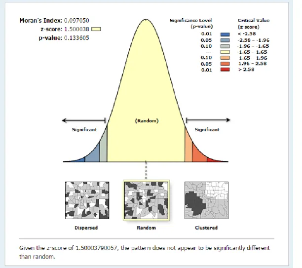
Figure 9 –Spatial autocorrelation analysis of the county level map (Figure 8)……….... 35
Figure 10 – North Carolina county level gastrointestinal illness map (quantiles)………... 36
Figure 11 – North Carolina ZIP code-level gastrointestinal illness map……… 37
Figure 12 – Spatial autocorrelation analysis of the ZIP code level map (Figure 11)…………... 38
Figure 13 – North Carolina norovirus map.……….. 40
Figure 14 – “High-Viral” vs. “Low-Viral” season maps……….... 41
Figure 15 – Incidence of gastrointestinal illness, split by age group………... 42
Figure 16 – Incidence of gastrointestinal illness, split by gender map……….... 43
Figure 17 – North Carolina county level gastrointestinal illness map overlaid with average household size……….. 44
Figure 18 – North Carolina county level gastrointestinal illness map overlaid with percent of population living below poverty level………... 45
Figure 19 – North Carolina county level map of rural-urban continuum codes (RUCC)……….. 46
Figure 21 – North Carolina county level gastrointestinal illness map
overlaid with health insurance type……….…… 49 Figure 22 – Monthly distribution of ED visits for gastrointestinal illness
after periods of heavy and light rain, both lag periods……… 53 Figure 23 – Map of average rates for light vs. heavy precipitation,
3-day lag period and proportional difference rates map...……….. 55 Figure 24 – Map of North Carolina drainage basins and proportional
10-day lag period counties highlighted that match basins ……….. 56 Figure 25 – Map of North Carolina river basins and highlighted areas of
LIST OF ABBREVIATIONS
AGI Acute gastrointestinal illness, including specified and non-specified
causes for illness, as derived from the ICD-9-CM codes 1.00-9.00 (specified gastrointestinal illness) and 589.89 (non-specified, noninfectious
gastrointestinal illness, including acute gastrointestinal illness) ArcGIS A geographic information system (GIS) for working with maps and
geographic information
CISA Carolinas Integrated Science Assessments, South Carolina
ED Emergency Department
EPA Environmental Protection Agency
ICD-9-CM International Classification of Diseases, Ninth Revision, Clinical
Modification. A set of standardized codes used to describe diagnoses of morbidity in hospitals.
IPCC Intergovernmental Panel on Climate Change
NC North Carolina
NC DETECT North Carolina’s statewide syndromic surveillance system, which is funded by the North Carolina Division of Public Health (NC DPH) Federal Public Health Emergency Preparedness Grant and managed through collaboration between NC DPH and the University of North Carolina at Chapel Hill’s Department of Emergency Medicine’s Carolina Center for Health Informatics
CHAPTER 1: ACUTE GASTROINTESTINAL ILLNESS AND DIARRHEA
Introduction: Gastrointestinal Illness and Diarrhea
One of the targets of the United Nations’ 2015 Millennium Development Goals was to “halve, by 2015, the proportion without sustainable access to safe drinking water and basic sanitation” (United Nations, 2008). Now in 2015, assessments of our progress have been made. Between 1990 and 2015, progress was made, as 2.6 billion people gained access to improved sources of water (United Nations, 2015). However, the United Nations reports that there are still 2.4 billion people that use unimproved sanitation facilities (United Nations, 2015), which can contribute to disease burdens in those communities (DeFelice, Johnston, & MacDonald Gibson, 2015). Diarrhea and gastrointestinal illness are illnesses that are often associated with poor drinking water and sanitation (Patz, Vavrus, Uejio, & McLellan, 2008). Despite uncertainties associated with all estimates of disease burdens, one detailed literature review has concluded that the median number of global annual deaths from diarrhea is 2.5 million people, which, although high, shows a decrease over four consecutive decades (Kosek, Bern, & Guerrant, 2003). Even with the decrease in
mortality from diarrhea, illnesses associated with the consumption of contaminated or inadequately treated water are still a global public health concern (Murphy et al., 2015b).
improvement of the municipal water and sewer systems in the United States during the twentieth century (DeFelice et al., 2015). The improvements in these United States’ public systems served as highly influential public health advances that helped contribute to decreased rates of infant mortality, child mortality, and total mortality during the twentieth century (DeFelice et al., 2015). However, drinking water is still responsible for a portion of all cases of acute gastrointestinal illness (AGI) in developed countries such as the United States (Murphy et al., 2015a).
The short period of time that it takes for most enteric and acute gastrointestinal illnesses, including diarrhea, to run their course makes them largely underreported in clinical records, both in the United States and globally (Drayna, McLellan, Simpson, Li, & Gorelick, 2010; Murphy et al., 2015b). However, research suggests that drinking water contributes an estimated 4.3-16.4 million cases of gastrointestinal illness (GI) in the United States annually (Colford et al., 2006; Messner et al., 2006; Tinker et al., 2010). Despite great efforts and many resources devoted to maintaining safe drinking water in the United States, there are still pathogens present in source waters that are used for drinking water purposes (Tinker et al., 2010) and there is some evidence to suggest that developed countries with established municipal and sewer systems are not entirely immune to diseases of this type (Murphy et al., 2015a). Users of private wells and small water systems may be at an increased risk of AGI (Murphy et al., 2015b). In the United States, private wells that are shallow may be especially prone to contamination (Richards et al., 1996). Gastroenteritis, diarrhea, and AGI, the disease outcomes of this study, are the primary diseases associated with contaminated water exposure (Patz et al., 2008). In 2003 and 2004, gastroenteritis (referred heretofore as gastrointestinal illness) was noted in 48% and 68% of reported recreational and drinking water outbreaks,
Disease Burden
Waterborne diseases are one of the major contributors to global disease burden and mortality (Pruss-Ustun, et al., 2014). Waterborne and foodborne disease outbreaks also contribute to significant morbidity in the United States. In 2002, there were 1,330 water-related disease outbreaks (Socolovschi, et al., 2011). In the cases associated with recreational water, bacteria were responsible for the most outbreaks (32%), parasites (mainly Cryptosporidium) accounted for 24%, and viruses accounted for 10% (Lowe, Ebi, & Forsberg, 2013). In drinking water outbreaks, bacteria were also the most responsible for outbreaks (29%, with Campylobacter as the most common bacteria), followed by parasites and viruses, which accounted for 5% each (Lowe et al., 2013).
Waterborne pathogens are associated with high rates of AGI and a small but significant number of deaths (Portier, Thigpen, Carter, & Dilworth, 2010). Waterborne diseases may cause as many as 900,000 cases and 900 deaths to occur annually in the United States (Bennet, Homberg, & Rogers, 1987). Gastroenteritis remains the primary disease associated with food and water exposure (Lowe et al., 2013). It has been estimated that up to 19 million cases of AGI may be due to
contamination of public drinking water systems (Colford et al., 2007; Messner et al., 2006; Reynolds, Mena, & Gerba, 2008). Children under the age of five and the elderly show the highest levels for risk of waterborne disease infection (Teschke et al., 2004), and often have higher incidence of
waterborne disease following heavy rainfall (Wade et al., 2004). The symptoms often associated with AGI range from mild to acute and include nausea, vomiting, and diarrhea (Rose et al., 2000).
Pathways to Human Exposure: Overview
Humans may be exposed to contaminated waters via a number of routes, one being
of the inhalation of particulates or volatiles or as a result of direct contact with contaminated water bodies or agricultural soils (Boxall et al., 2009). Direct contact with contaminated floodwaters via walking or swimming can also cause illness (Greenough et al., 2001; Malilay, 1997). Ear, nose, and throat, respiratory, and gastrointestinal illnesses are frequently associated with recreational swimming in both fresh and oceanic waters (Lowe et al., 2013). Swimmers have a greater risk of contracting gastrointestinal illnesses than non-swimmers, and this risk has been shown to increase with prolonged exposure (Lowe et al., 2013). Heavy runoff after severe rainfall can also contaminate recreational waters, increasing the risk of human health impacts with higher bacterial counts (Lowe et al., 2013). This association has been found to be most closely associated at the beaches that are closest to rivers (Lowe et al., 2013).
The largest waterborne disease outbreak ever to impact the United States occurred in 1993 in Milwaukee, Wisconsin, and was a result of outdated combined sewer system infrastructure (MacKenzie et al., 1994). In the wake of the heaviest rainfall the region had received in over 50 years, a parasitic Cryptosporidium outbreak occurred as the combined sewer system sent sewage directly into local surface waters (MacKenzie et al., 1994). The Cryptosporidium infections affected more than 400,000 people and caused over 100 deaths (MacKenzie et al., 1994). Symptoms of that outbreak included severe diarrhea that lasted from several days to a week (MacKenzie et al., 1994). Similarly, Cryptosporidium transmission in humans has been linked to agricultural areas where manure is applied to land as a fertilizer (Lake et al., 2007). Waterborne disease outbreaks from the
Pathways to Human Exposure: The impact of Heavy Rains on Drinking and Recreational Water Contamination
Just as the 1993 Cryptosporidium outbreak followed the heavy rainfall event in Milwaukee (MacKenzie et al., 1994), over 60% of waterborne disease outbreaks have been shown to be preceded by precipitation events above the 90th percentile (Curriero, Patz, Rose, & Lele, 2001). After heavy precipitation events, floodwaters can contain over 100 types of disease-causing bacteria, viruses, and parasites (Batterman et al., 2009; Domino, Fried, Moon, Olinick, & Yoon, 2003; Rose et al., 2000). Moreover, a storm surge can infiltrate human infrastructure from the sea, and/or the build-up of agricultural waste, human waste, and chemicals can subsequently mix with freshwater sources. The rate and effect to which runoff of storm water can happen depends on multiple variables, such as slope, vegetation, flow rate, infiltration rate, and rainfall intensity (Sterk, Schijven, de Nijs, & de Roda Husman, 2013).
In some older cities, like Milwaukee, the contamination leading to such waterborne disease outbreaks can be attributed to combined sewer systems, wherein during an overflow event,
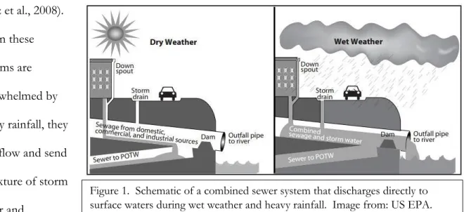
When the water volume exceeds the containment capacity of the water treatment plant, the overburden is typically discharged directly into surface water bodies (Patz et al., 2008). The cities with combined sewer systems are the most at risk from the threat of water contamination and include more than 700 communities throughout the nation (EPA, 2011). Combined sewer systems are designed to collect both sanitary sewage and storm water (Patz et al., 2008). These systems then transport the sewage and storm water to a wastewater treatment plant, where they are all treated (Patz et al., 2008).
When these systems are overwhelmed by heavy rainfall, they overflow and send a mixture of storm water and
untreated raw
sewage directly into surface waters and local waterways (Curriero et al., 2001). The excessive rainfall can cause the untreated sewage in combined systems to breach the dam (sometimes called weir) and then to be mixed directly with the storm water that is released into surface waters (Figure 1, EPA 2004).
Obviously, this risk varies greatly depending on each individual system and regional differences. For example, more than 2.5 inches of rainfall in one day in the Chicago area will send raw sewage into Lake Michigan, whereas .25 of an inch in Indianapolis can send raw sewage into surface waters (Hayhoe & Wuebbles, 2008). Regardless of regional variations, the national toll of combined sewer systems is grand: each year, overflows from combined sewer systems can send over
850 billion gallons of stormwater and sewage into local waterways (EPA, 2004). This can be particularly dangerous for communities with recreational facilities along the surface waters and coastal beaches where people swim. At the time of writing, the majority of the communities served by combined sewer systems were concentrated in the Midwest and the Northeast, and there were no combined sewer systems in North Carolina (EPA, 2004, Figure 2).
2001). Although the literature suggests that rainfall alone is not predictive of an outbreak, heavy rainfall may increase the potential for disease exposure, which could lead to an increase in the potential risk to public health. In sum, the issue of disease as a result of contaminated water is absolutely one that merits further research. In fact, the United States Environmental Protection Agency (EPA) stated in 1990 that “microbial contamination from pathogens represents the greatest remaining risk to drinking-water supplies” (Macler & Merkle, 2000).
Links between precipitation and gastrointestinal illness, AGI, and diarrhea
After a heavy rainfall event, floodwaters can be contaminated with over 100 types of disease-causing agents (Batterman et al., 2009). These disease-disease-causing agents can come in many different forms, including viruses, bacteria, and protozoans (Drayna et al., 2010). The majority of the viral agents (e.g. rotavirus, norovirus, enterovirus, calcivirus, and adenovirus) that can cause
gastrointestinal illness, AGI, and diarrhea have incubation times from 1-7 days (American Academy of Pediatrics, 2006; Drayna et al., 2010). Bacterial causes of gastrointestinal illness, AGI, and diarrhea are much less common, but have similar incubation times to viral agents (Drayna et al., 2010). Examples of bacterial causes of gastrointestinal illness, AGI, and diarrhea include
Campylobacter sp., Salmonella sp., and Echerichia coli sp. Protozoans have longer incubation periods than
Escherichia coli (E. coli), which is a type of bacterium that typically originates in the intestines
of humans and some other mammals, can also cause gastrointestinal illness (Batterman et al., 2009). E. coli has been found in storm water at concentrations of 100 to 500 times higher than the
maximum water quality standards in Lake Michigan after heavy rains (McLellan et al., 2007). After five days of heavy rain Walkerton, Ontario in 2000, high concentrations of E. coli in the water supply also caused over 2,300 cases of illness and seven deaths (Auld, MacIver, & Klaasen, 2004). Once considered only a foodborne pathogen, E. coli continues to be linked to waterborne disease. In fact, the largest reported outbreak of E. coli 0157:H7 occurred at a fairground in New York State in September of 1999 and it was linked to contaminated well water (Curriero et al., 2001). Furthermore, the unusually heavy rainfall linked to this outbreak was preceded by a drought
(Curriero et al., 2001; Patz et al., 2000). Several articles document increases in diarrhea or outbreaks following dry periods, which might suggest an interaction between the accumulation of pathogens in the environment during dry periods (referred to as the “concentration effect”) followed by rain events that can then spread the accumulated pathogens (Adkins et al., 1987; Carlton et al., 2014; Effler et al., 2001; Nicholas, Lane, Asgari, Verlander, & Charlett, 2009; Smith et al., 1989; Willocks et al., 1998).
In addition to E. coli, other bacteria are frequently associated with waterborne disease outbreaks. Vibro sp. are one of the most-frequently associated waterborne bacteria with heavy precipitation (Schwab, 2007). Vibrio are ubiquitous, heterotrophic bacteria (Schwab, 2007) and its genus includes three significant human pathogens: Vibrio cholera, Vibrio parahaemolyticus, and Vibrio vulnificus (Schwab, 2007). According to leading scientists, “all three species have been demonstrated
Coast estuaries (Shope, 1991) and could therefore be a future threat to some eastern United States’ watersheds, such as those in the state of North Carolina.
Temperature is a limiting factor for Vibrio (Shope, 1991). Total Vibrio abundance is typically high in the summer and low (sometimes undetectable) in the winter months or when temperatures fall below 10-12ºC (Shope, 1991). Salinity is also a limiting factor for Vibrio growth, and mesohaline waters are optimal for growth (Schwab, 2007). Very high or very low salinities have been shown to be detrimental to Vibrio growth and development (Schwab, 2007).
The consequences of increased Vibrio exposure to humans in a climate that is projected to be warmer, wetter, and potentially less saline (due to increased precipitation, increased valley-glacier melt into surface water bodies, and increased continental-glacier melt into oceans) could be
significant. Scientific observations have raised questions about the ecological response of total Vibrio, which could see major changes in a warming climate. Although one species may not seem
like much, even small increases in risk, if left unchecked, could represent substantial impacts to the global burden of disease.
It has been well-documented that water in general and floodwaters specifically can spread pathogens within watersheds (Curriero et al., 2001; Dorner, Anderson, Slawson, Kouwen, & Huck, 2006; Ferguson, Husman, Altavilla, Deere, & Ashbolt, 2003). Excessive rainfall can mobilize pathogens in the environment and contribute to an increase in runoff from livestock or other agricultural fields, as well as transport them into rivers, coastal waters, and wells (Semenza et al., 2009). Waterborne disease outbreaks in the U.S. are clustered in key watersheds and associated with heavy precipitation (Patz et al., 2008).
runoff have been associated with individual outbreaks of waterborne disease caused by fecal-oral pathogens (Rose et al., 2000). Fecal-oral pathogens, which originate from human or animal wastes, include the following: bacteria (Escherichia coli (E. coli), Campylobacter, Salmonella, and Shigella), viruses (Norwalk virus, small round structured viruses, and hepatitis A virus), and protozoa (Cryptosporidium and Giardia) (Rose et al., 2000). Rose et al. (2000) also confirmed a statistically significant
relationship between precipitation events and waterborne disease outbreaks originating from groundwater sources (Rose et al., 2000). In brief, there is mounting evidence that heavy precipitation and runoff events add to the risk of waterborne disease outbreaks (Curriero et al., 2001).
Connection to Climate Change
During the 20th century, greenhouse gas concentrations have increased significantly (IPCC, 2013; Nicholls & Cazenave, 2010). The burning of fossil fuels has been a major contributor to this rise in greenhouse gas concentrations, and there is increasing scientific data to support that the human-caused (anthropogenic) emissions of greenhouse gases are having a noticeable impact on the climate of the Earth (Houghton, 2009). Global temperatures have been observed as having
increased 0.6ºC and global sea levels have risen 10-20cm (Houghton, 2009). This anthropogenic influence on climate is expected to increase during the 21st century and beyond (IPCC, 2013).
This regional and geographic hydroclimatic variability can make specific projections of future climate change impacts difficult (IPCC, 2013). In the United States, data show that downpours averaged less than 8 percent of the total annual precipitation at the beginning of the twentieth century and that they had increased to 10 percent of the total at the end of the century (Rose et al., 2000).
This meteorological variability is not unique to the present, as it can also be observed in climate reconstructions of the past. Scientists are still trying to find trends and patterns regarding historical extreme weather-related events. According to the most recent IPCC report (the
Assessment Report Five, often referred to as the AR5, released in 2013/2014), regional trends in precipitation extremes since the middle of the 20th century are varied. Nonetheless, there are some distinct weather patterns that can be extracted from long-term data despite the regional variation. It is likely that since 1951, there have been increases in the number of heavy precipitation events in more regions than there have been decreases (Trenberth, 2011). However, Trenberth also
acknowledges that there are strong regional and subregional variations in these trends and that not all regions of the United States will experience a wetter and rainier future (Trenberth, 2011).
weather will be of a wetter and rainier overall nature, however these trends could have regional variability (Alexander, 2009; Trenberth, 2001; Westra et al., 2013).
With the expectation of meteorological changes that could include an increase in precipitation in at least some parts of the United States, the US National Assessment on the Potential Consequences of Climate Variability and Change has stated that “determining the role of weather in the incidence of waterborne disease outbreaks is a priority public health research issue for this country” (Curriero et al., 2001).
Overall Objectives of the Study
The overall objective of this study is to uncover spatial and temporal patterns of diarrheal disease across the state of North Carolina and to determine if those patterns are related to
socioeconomic, demographic, and/or meteorological factors. North Carolina is a good study area for multiple reasons. The state has distinct geographic variation that includes mountains, piedmont, and coastal areas, which can contribute to variations both in meteorology as well as variations in the incidence of gastrointestinal illness, AGI, and diarrhea across the state. In addition to geographic variability, there is a wide range of variation in the demographic and socioeconomic statuses across the state of North Carolina (Sugg et al., 2015). Some of these variations may also be associated with incidence of disease across the state.
Although waterborne disease outbreaks are frequently associated with heavy precipitation events, this study will establish North Carolina baseline levels for diarrheal disease infections that may not be classified as “outbreaks,” but can still be associated with rainfall trends and patterns. As such, we hope that the results of this study may be able to inform health officials in specific counties of a potential increase in number of waterborne disease infections given a particular set of
been determined, this could be used as real-time information to guide better prevention and controls to limit the impacts or magnitudes of contamination events for the state (Patz et al., 2008).
CHAPTER 2: METHODS
Data Sources and IRB Exemption
Data sources for this study include the NC DETECT (North Carolina Disease Event Tracking and Epidemiologic Collection Tool), the United States Bureau of Census including the American Community Survey (ACS), a previously-published study that determined drinking water sources (private or community systems) at the county-level for the state of North Carolina (Luh et al., 2015), and weather stations maintained by the National Weather Service and Federal Aviation Administration (FAA) and the U.S. Forest Service (USFS) as well as stations in the North Carolina Environment and Climate Observing Network (NC ECONET). This research project was
approved as exempted research by the University of North Carolina Institutional Review Board (IRB) (Study number 15-1158).
Health Data
Incidence of gastrointestinal illness, AGI, and diarrhea in North Carolina was determined using Emergency Department (ED) visit data from NC DETECT (North Carolina Disease Event Tracking and Epidemiologic Collection Tool), and the methodology for the data extraction emulated a previous study on heat-related illness in North Carolina (Sugg, Konrad, & Fuhrmann, 2015). NC DETECT is North Carolina’s statewide syndromic surveillance system, which is funded by the North Carolina Division of Public Health (NC DPH) Federal Public Health Emergency
North Carolina at Chapel Hill’s Department of Emergency Medicine’s Carolina Center for Health Informatics.
When the ED visits are reported to NC DETECT, the reason for patient admission is coded via ICD-9-CM code into the NC DETECT database upon patient discharge. For the purpose of this study, we followed a version of the case definition for gastrointestinal illness from previous literature and used the ICD-9-CM codes (International Classification of Diseases, 9th Revision, Clinical
Modification) shown in Table 1. Heretofore, we will use the term “gastrointestinal illness” and/or
“gastrointestinal disease” interchangeably as an umbrella term to describe results for all of the ICD-9-CM codes utilized in this study (Table 1). We chose to exclude nausea with vomiting (787.01-787.03) as well as abdominal pain (789.0) in our case definition to increase the specificity of the case
definition. Following existing literature (Tinker et al., 2010), we included non-infectious gastrointestinal illness (558.9) due to the fact that research has shown that some cases of actual gastrointestinal illness cases are misclassified into this diagnostic code (Gangarosa, Glass, Lew, & Boring, 1992; Hoxie, Davis, Vergeront, Nashold, & Blair, 1997; Schwartz, Levin, & Hodge, 1997; Tinker et al., 2010). Furthermore, some care providers may choose not to run specific tests on intestinal infectious diseases (codes 001-009) (Tinker et al., 2010) due to cost, time constraints, or other reasons, meaning that actual intestinal infections that could be specified (e.g. norovirus, salmonella, etc.) get coded instead as “non-specified.”
ICD-9-CM
Diagnosis Code Disease Examples (incomplete list)
001-009 Intestinal infectious diseases
Cholera (001)
Salmonella (003)
Giardiasis (007.1)
Cryptosporidosis (007.4)
Campylobacter (008.43)
Norovirus (008.63)
Rotavirus (008.61)
558.9
Gastroenteritis, noninfectious,
unspecified
Acute gastroenteritis Enteritis
Gastroenteritis 787.91 Diarrhea, not otherwise
specified
Diarrhea, noninfectious Nausea, vomiting and diarrhea
Emergency Department (ED) visit data have been used as a uniform sentinel for
community-wide events of gastrointestinal illness in similar contexts before (Drayna et al., 2010; Tinker et al., 2009) and thus provide a framework to follow in this North Carolina-based study. In addition to providing the ICD-9-CM code that describes the reason for each ED visit, NC
such as age, gender, county of residence and ZIP code of residence for the patient. Each visit can be linked to as many as 11 ICD-9-CM diagnoses codes. Similar to the heat-related illness studies after which this study was modeled (Lippman et al., 2013; Sugg et al., 2015), ED visits containing at least one code from Table 1 were used to calculate the incidence of gastrointestinal illness in North Carolina during the study period, regardless of if those codes were categorized as primary or secondary codes.
Due to the fact that the NC DETECT data is only ED visits, the data could be skewed based on multiple factors, such as gender [many ED data studies have found that, in general, women frequent the Emergency Department more often than men, (Agency for Healthcare Research and Quality, 2011)] and severity of illness (Lowe et al., 2003). Other limitations with ED data could include, but are not limited to, a lack of individual data regarding disease etiology, clinical course, drinking water source and habits, and recreational water exposures (Drayna et al., 2010).
Furthermore, considering that ED data itself can present an underestimation of the true incidence of disease (Drayna et al., 2010), all 11 possible codes (both primary and secondary diagnoses codes) were utilized in order to capture a larger proportion of ED visits. In this North Carolina-based study over a five-year period (2008-2012), the resulting dataset contains a total of 660,891 ED visits for the ICD-9-CM codes shown in Table 1.
Demographic Data
population estimates were used as denominators in the estimation of gastrointestinal illness ED visits per 100,000 person years (modeled after Sugg et al., 2015). Corresponding to the 2010 US Census age categories, all 660,891 cases were divided into 12 age categories in order to obtain the rates for different age groups and demographic groups (i.e. under 5, 5 to 9, 10 to 14, 15 to 17, 18 to 24, 25 to 34, 35 to 44, 45 to 54, 55 to 64, 75 to 84, and over 85).
In addition to age and gender, we assessed whether other measures of demographic and socioeconomic character factor into the incidence of gastrointestinal illness. We chose to determine if there were associations between gastrointestinal illness in North Carolina counties with the
following elements: percentage of the population living in poverty (divided into two age categories by the U.S. Census Bureau: under 18 and 18 to 64), average number of people per household, urban vs. rural counties, drinking water source, and the type, level, and percentage of health insurance coverage. All of the information for the above elements was collected from the 5-year estimates in the American Community Survey for 2008-2012 at the county level (methodology modeled after Sugg et al., 2015; data from United States Census Bureau 2006-2010).
Drinking water source data by county for the state of North Carolina were obtained from a previous study conducted at the University of North Carolina at Chapel Hill through the Gillings School of Global Public Health (Luh et al., 2015). The authors of that study calculated the
proportion of the county population serviced by different water technology types (Luh et al., 2015). In order to do so, they assumed that the only two water technology types in the United States were domestic self-supply (private wells) and community piped water systems as defined by the United States Environmental Protection Agency (EPA) (Luh et al., 2015; USEPA 2012).
recognize that there could be discrepancies in this information since the private well information provided by Luh et al. (2015) is from 2005 and our study runs from 2008-2012. However, we assumed that the variation in the percentage of the population using self-supplied vs. community water systems from 2005-2008 would not be so great as to egregiously skew the results for the study. Secondly, Luh et al. (2015) obtained county-level information on the number of people on very small, small, medium, large, and very large community piped water systems in 2010 from the U.S. EPA Safe Drinking Water Information System (SDWIS) (Luh et al., 2015; USEPA, 2012), wherein the size categories are determined based on the size of the population served (Luh et al., 2015). We were given access to this North Carolina county-level drinking water-source data in early November 2015 to include in our study.
Meteorological Data
accepted lag period in the existing literature (Drayna et al., 2010; Tinker et al., 2010). We chose for the precipitation data available within the NC DETECT Climate-Health Toolbox to pull from the following weather networks: the Automated Surface Observing System (ASOS), the Automated Weather Observing System (AWOS), and the North Carolina Environment and Climate Observing Network (ECONET). In total, there are 113 of these stations across the 100 counties in North Carolina (Sugg et al., 2015). The patient’s county of residence was utilized to determine which weather station to assign to each ED visit. If nearby weather stations were missing precipitation data or not functioning at the time of the ED visit, the closest weather station with available data was assigned to the ED visit.
Within the Climate-Health Toolbox, the ZIP code of the patient’s residential address was utilized to determine which weather station to assign to the ED visit. The nearest weather station was identified using the center of the patient’s ZIP code area to determine the shortest distance to a station. This was based on the Euclidean distance using the great circle distance formula:
D = R cos-1 [sinl
1 sinl2 + cos l1 cosl2 cos (m2—m1)]
where D is the distance (km) between the ED patient’s residence and the weather station, R is the mean earth radius, l1 and l2 are latitudes (rad) of the ED patient’s residence and the weather station,
respectively, and m1 and m2 are the longitudes (rad) of the ED patient’s residence and the weather
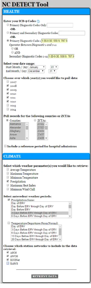
Figure 4. Features of the NC DETECT Climate-Health Toolbox. This example shows how information for this study was retrieved from the NC DETECT ED visit database and the North Carolina weather station networks.
Once the meteorological data was extracted from the NC DETECT Climate-Health
Toolbox, we isolated the information just to examine a 3-day lag and a 10-day lag for the purpose of this study. An example for the Climate-Health Toolbox parameters of a “lag period” is that, using a 3-day lag as an example: a 3-day lag is the sum of all of the precipitation that occurred three days before the ED visit up until the day of the visit, including the precipitation data from the date of the visit itself. Similarly, a 10-day lag represents the sum of all of the precipitation beginning ten days prior to the ED visit and including all of the days leading up to visit and the precipitation data from the date of the visit itself. We recognize that there are limitations associated with this definition, including the following: 1) other lag periods may capture a different relationship and 2) the
precipitation can occur in the hours after a patient enters the emergency room. The module in the NC DETECT Climate-Health Toolbox that estimates precipitation for each visit is still under development, and as such the tool is currently being updated based on feedback from studies like this one. Future studies will be able to use this module to explore a wider range of precipitation lags and therefore identify the one that best captures the relationship.
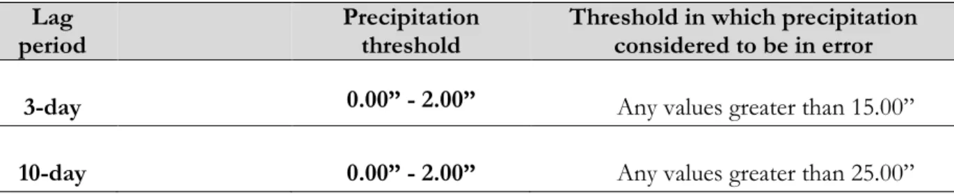
Lag period
Precipitation threshold
Threshold in which precipitation considered to be in error
3-day 0.00” - 2.00” Any values greater than 15.00”
10-day 0.00” - 2.00” Any values greater than 25.00”
The following information was calculated for each lag period and precipitation group: 1) Cases per county over the entire study period (2008-2012)
2) The average cases per county
3) The average rate of ED visits per county per 100,000 person-years
4) The proportional difference between the heavy and light precipitation groups 5) The average rate of ED visits across the entire state per 100,000 person-years
Cases per county over the entire study period were derived by using a Pivot Table in Excel that summed the cases per county from the originally-extracted data, which was already sorted based on the given lag period of interest. Using that cases per county information, the average cases per county was calculated (e.g., the cases per county were divided by how many days the condition (heavy or light) was observed). The information regarding how many days in the study period had observations of heavy or light precipitation, given both lag periods, was provided by the North Carolina State Climate Office (SCO). The leap days both in 2008 and in 2012 were taken into account when measuring the number of days in the 5-year study period that the certain conditions were observed.
Next, the rate of average ED visits per county per 100,000 person-years was calculated by dividing the average cases per county values by the population per county (based on the U.S. Census
data) and then multiplying by 100,000. These values, although still in 100,000 person-years, are smaller than previous values throughout the study for 100,000 person-years due to the fact that the average number of cases per county was divided by the population whereas earlier calculations were
made by dividing total number of cases per county by the population of respective county. The rates of average ED visits per county per 100,000 person-years were mapped for both lag periods and precipitation groups using the ArcMap product within ArcGIS10.2. The map scales for each lag period are the same; to see maps with natural breaks used to delineate contour values (Jenks), refer to Appendix 3.4.
Proportional differences between the two rates of average ED visits per county per 100,000 person years for the rain thresholds (heavy vs. light) were then determined. These proportional differences were calculated for the heavy and light rates within each given lag period. Proportional rates were determined simply by dividing the heavy rates by the light rates. Those proportional differences were then mapped for both the lag periods using ArcGIS10.2 to show whether or not average ED visits per county per 100,000 person-years were higher after heavy rain totals.
Furthermore, we hypothesized that counties with the biggest proportional increases could be related to waterborne disease vulnerability. T-tests for both lag periods were also carried out to determine the statistical significance of the proportional differences results.
Geographic Data
North Carolina has distinct physical geographical regions (e.g. mountains, piedmont, and coastal plain) that are hypothesized to contribute to variations in the incidence of gastrointestinal illness across the state. In addition to geographic variability, there is a wide range of variation in the demographic and socioeconomic statuses across the state of North Carolina (Sugg et al., 2015). Some of these variations may also be associated with incidence of gastrointestinal illness across the state. We chose to ascertain the rurality of North Carolina counties in this study and did so using the Rural-Urban Continuum Codes (RUCC) provided by the United States Department of
Agriculture, Economic Research Service (USDA, 2013). According to the Rural-Urban Continuum Codes, rurality is measured based on metropolitan vs. nonmetropolitan areas, and then population size per county. The Rural-Urban Continuum Codes are developed for the entire United States and the specific qualifications for each code are listed below in Table 3. We chose to investigate rurality because we suspected that there might be an association between runoff from livestock and
Code Description
Metro counties:
1 Counties in metro areas of 1 million population or more 2 Counties in metro areas of 250,000 to 1 million population 3 Counties in metro areas of fewer than 250,000 population Nonmetro counties:
4 Urban population of 20,000 or more, adjacent to a metro area 5 Urban population of 20,000 or more, not adjacent to a metro area 6 Urban population of 2,500 to 19,999, adjacent to a metro area 7 Urban population of 2,500 to 19,999, not adjacent to a metro area
8 Completely rural or less than 2,500 urban population, adjacent to a metro area 9 Completely rural or less than 2,500 urban population, not adjacent to a metro area
Mapping of Spatial Patterns
Spatial patterns of incidence of gastrointestinal illness across the state of North Carolina were assessed at the county and ZIP code level. Gastrointestinal disease rates per 100,000 person-years were mapped using the ArcGIS 10.2 product within ArcMap. Maps expressing rates in 100,000 person-years were made using the “Jenks method,” a classification method proposed by George Jenks and collaborators in the 1970s (Jenks and Caspall, 1971; Jenks, 1977). The “Jenks method,” sometimes referred to as the Jenks optimization method or the Jenks natural breaks classification method, is a method of data classification that determines the best arrangement of values into different classes (Chen et al., 2013). This is accomplished by minimizing each class’
average deviation from the class mean and simultaneously maximizing each class’ deviation from the means of the other groups (Chen et al., 2013).
The 2008-2012 incidence rates per 100,000 person-years using the “Jenks method” was utilized as the uniform standard for comparison and/or serves as the baseline map for all other maps. As a result, different years, age groups, and various socioeconomic factors can all be
compared to the uniform standard. Unless otherwise noted, the rates on the maps are based off of the 5-year study period uniform standard.
Statistical Analyses
The overarching objective of this study was to document patterns of gastrointestinal illness in space and time and determine how these patterns relate to socioeconomic, demographic factors and precipitation. Within that overarching objective, we hoped to identify relationships between heavy precipitation and incidence rates of gastrointestinal illness. Various statistical analyses were performed in this study to quantify the geographic variability of illness and assess the nature of its relationships with certain socioeconomic and demographic factors. These analyses are described below.
T-tests were used to ascertain the statistical significance of differences in rates of gastrointestinal disease across different groups (e.g. cases associated with heavy vs. light
precipitation). Correlations were calculated to assess the strength of relationship between different variables in the study. Correlations were identified using the Microsoft Excel 7 program,
Moran’s I provides a measure of the degree of spatial autocorrelation and was used to
CHAPTER 3: RESULTS
Introduction
Emergency Department, meteorological, and population data were all analyzed in order to assess the spatial and temporal patterns of gastrointestinal disease across the state of North Carolina. Results are conveyed in the form of maps, correlation matrices, correlograms, as well as summary tables and charts.
Descriptions of temporal patterns
Gastrointestinal illness Emergency Department visits show one spike for total counts around 10:00am and another spike around 7:00pm (Figure 5). The 10:00am spike in Emergency Department visits coincides with reported visit escalations at that time for all Emergency
Total counts: 660891
Figure 7. Total Counts of gastrointestinal illness, AGI, and diarrhea in North Carolina from 2008-2012, separated by day of year.
Figure 6. Total Counts of gastrointestinal illness, AGI, and diarrhea in North Carolina from 2008-2012, separated by month of year.
Spatial patterns
The incidence rates per 100,000 person-years of gastrointestinal illness ED visits by county are presented in Figure 8. The highest rates of gastrointestinal illness were found in the following counties using the “Natural Breaks” (Jenks) method, shown West to East (Figure 8): McDowell (2,856.6), Anson (2972.4), Halifax (2,966.5), and Chowan (2,586.4) counties.
Spatial autocorrelation tests for the overall county-level “Natural Breaks” map were run using the Moran’s I calculation and results show that at a 95% confidence interval, there is no significant clustering at the county level (Figure 9). To examine spatial patterns over time, county-level maps for all individual years were made using a standard set of values for Natural Breaks; those can be found in Appendix 3.1.
When broken into quantiles (20 counties in each quantile) as opposed to natural breaks, incidence rates for gastrointestinal illness can be seen in more condensed areas of the state, despite a lack of statistical clustering (Figure 10). However, the .133 p-value does show that the value is right on the edge of being statistically significant at the 95% confidence interval, and therefore a smaller-scale of observation, such as a map made at the ZIP code level, could show significant clustering. To examine spatial patterns over time, county-level maps made using a quantiles for all individual years in the study period can be found in Appendix 3.2.
Figure 9. Spatial autocorrelation analysis of the county-level map (Figure 7) for
gastrointestinal illness ED visits per 100,000 person-years from 2008-2012. Given the z-score and p-value for the map, the pattern does not appear to be significantly different from
A mapping of the patterns of gastrointestinal illness at the ZIP code level reveals a clustering in the pattern of incidence rates (Figure 12, which is revealed in the Moran’s I calculation) (Figure 11). The z-score indicates that there is a less than 1% likelihood that the clustered pattern could be the result of random chance (Figure 12). Although the statistical significance for clustering is highest at the ZIP code level, many of the calculations for this study were made at the county level (e.g. see the Study limitations portion of the Discussion section). The clustering of high rates at the ZIP code level is found largely in rural areas in the coastal plain as well as in scattered pockets in the Piedmont and the North Carolina mountains (Figure 11).
Figure 11. North Carolina ZIP code-level gastrointestinal illness ED visits per 100,000 person-years from 2008-2012. ED data are acquired through the NC DETECT. Data not available for ZIP code areas that are blank. The East coast blank areas are North Carolina sounds
Efforts were made to assess the effect of norovirus, an endemic disease that occurs year-round but has a pronounced winter peak and that may have a large influence on the geographic patterns of gastrointestinal illness (Hall et al., 2013). Despite causing an average of 400,000 emergency department visits in the United States each year and being recognized as “the leading
Figure 12. Spatial autocorrelation analysis of the ZIP code-level map (Figure 11) for
cause of epidemic acute gastroenteritis across all age groups,” norovirus has been poorly directly associated with respect to disease incidence (Hall et al., 2013). In the United States, there is
currently no public health reporting requirement for individual cases of norovirus (Hall et al., 2013). CalciNet, which is an outbreak surveillance network for norovirus in the United States, was
launched in March 2009 in an effort to “develop and improve standardized typing of norovirus outbreaks” (Vega et al., 2011). Although all 50 states have the laboratory capacity for testing norovirus, unfortunately for this study, as of 2011, North Carolina was not a participating state in CalciNet (Vega et al., 2011).
Seasonal maps were made to see if the geographical patterns during the cool season (October – March), when norovirus incidence is high, are different from the warm season (April – September), when bacterial agents may play a greater role for gastrointestinal illness. Hereafter, we refer to the former as “high viral” season where the rates are higher (e.g. Figure 6) and the latter as the “non-viral” season. The geographic patterns of disease incidence are very similar across the two seasons (Figure 14). As is expected, the signal for gastrointestinal illness is stronger in the high viral season; however, there are still some counties in the low-viral season that show high rates of gastrointestinal illness incidence, such as (from West to East) Caldwell, Anson, Robeson, Columbus, Halifax, Craven, and Chowan counties (Figure 14). The higher incidence rates in these counties could merit further investigation as to the potential sources of gastrointestinal illness increases there during the low-viral season (Figure 14).
Figure 14. High Viral vs. Low-Viral Season Maps: county-level maps for gastrointestinal illness ED visits per 100,000 person-years from 2008-2012.
High Viral Season Rates of AGI, 2008-2012
Demographic patterns
Demographic information results display information gathered in terms of gender and age, both from NC DETECT and the US Census. Additional information gathered at the county-level from the US Census included average household size, poverty status, urban or rural, proportion of residents using specific sources of drinking water, and health insurance status. As is consistent with existing literature regarding the use of the ED for all causes (Agency for Healthcare Research and Quality, 2011), more women than men visited the ED for gastrointestinal illness, as women
comprised roughly 60% of the visits for gastrointestinal visits, while men accounted for only 40%. This study also supports existing literature that children under the age of five and the elderly show the highest levels for risk of waterborne disease infection (Teschke et al., 2004), as those two age groups show the highest incidence rates for gastrointestinal disease in this study (Figure 15).
The geographic patterns of gastrointestinal disease at the county level are similar across gender (Figure 16). Age group maps using a standardized scale show a wide range of variation among incidence rates of gastrointestinal illness across age groups and geographic counties, with the under 5 and over 85 age groups reflecting the highest incidence rates of disease (Appendix, 3.2). Maps generated with more specific breakdowns (natural breaks) for age groups that showed some of the highest rates (under 5, 18-24, 35-34, and over 85) also show county level spatial incidence rates (Appendix 3.3).
Females
Males
A map of the state for average household size within each county shows that there are some distinct geographic pockets across the state with larger average household sizes (Figure 17). This measure was selected since it could be a confounding factor for the spread of disease, specifically diarrheal disease, within homes that have more people per household. Although all of the counties in the highest disease bracket show average household sizes of 2.5 or greater, not all of the counties in the Sandhills within the second-highest disease bracket show this association (Figure 17).
Poverty shows much variation across the state but is especially clustered in the Coastal Plain and the Sandhills (Figure 18). Many of these counties (Anson, Halifax, Robeson, Columbus, Bladen, etc.) also display relatively high rates of gastrointestinal illness (Figure 18). Correlations for these variables at the end of this section reveal that some of the strongest relationships exist between poverty and incidence rates of disease (Table 4).
A rural and urban county-level map made utilizing the 2013 Rural-Urban Continuum Codes (RUCC) shows the urban and rural counties in North Carolina that could factor into incidence levels of gastrointestinal illness. Many, although not all, of the counties that are especially rural also display relative high rates of gastrointestinal illness (e.g. compare Figures 8 and 19).
Drinking water source maps for the state of North Carolina (Figure 20) show the proportion of the population in counties that use self-supplied drinking water, small or very small community systems, and medium, large, or very large community systems. The counties with the highest proportions of self-supplied drinking water are in the mountains region, which do not show the highest rates of gastrointestinal disease incidence. McDowell County is one of the four counties within the highest bracket for gastrointestinal disease incidence, and it has a 0.59-0.86 proportion of the population with self-supplied drinking water (Figure 20), but three of the other four highest disease-bracket counties have high proportions of their populations on community water systems (Figure 20).
Figure 20. Proportion of the population in each county using self-supplied drinking water (top), on small or very small community water systems (middle) and on
A correlation matrix supports the spatial results for demographic variables (Table 4). The only strong association with rates of gastrointestinal illness ED visits and a demographic variable is with the cluster of variables that relate to poverty, which includes percent of the population without health insurance or with only public health insurance (Table 4). The highest association (.40) within this poverty cluster is for the percent of the population under the age of 18 living in poverty (Table 4). The association for percent of the population aged 18-64 living in poverty is slightly lower, with a correlation rate of .24 (Table 4). The second-highest association (.35) is with the percent of the population that either has no health insurance or only public health insurance (Table 4).
Surprisingly, there is a negative correlation (-0.06) between rates and the proportion of the
R ate s A vg. Hs hold. S iz e % P ov: U nder 18 % P ov: 1 8-64 Hig h-V iral Se as on L ow -V iral Se as on DW : Se lf DW : S, V S DW
: M, L
, V L % No Hea lth I ns . % No or P ublic Hea lth Ins .
Rates 1.00
Avg. Hs. Size
0.02 1.00
% Pov.: Under 18
*0.40 0.06 1.00
% Pov.: 18-64
*0.24 -0.11 *0.71 1.00
High-Viral
*0.96 0.00 *0.42 *0.26 1.00
Low-Viral
*0.96 0.00 *0.36 *0.23 *0.97 1.00
DW: Self -0.06 -0.17 0.01 0.02 -0.09 -0.07 1.00
DW: S,VS
0.04 -0.24 *0.25 *0.22 0.07 0.01 0.10 1.00
DW: M, L, VL
0.03 *0.25 -0.12 -0.11 0.05 0.06 -0.89 -0.54 1.00
% No HealthIns
*0.23 -0.16 *0.40 *0.38 *0.27 *0.24 *0.21 *0.30 -0.31 1.00
% No or Public HealthIns
*0.35 -0.18 *0.73 *0.53 *0.38 *0.35 *0.29 *0.30 -0.38 *0.63 1.00
Table 4. Correlation Matrix for Rates of gastrointestinal illness per 100,000 person-years and demographic variables. A * represents statistical significance.
Key for abbreviations in Correlation Matrix:
Rates: Gastrointestinal illness ED visits per 100,000 person-years Pov.=Poverty
DW: Source of Drinking Water, value is proportion of population of county Self: proportion of population of county that is on self-supplied drinking water S, VS: proportion of population of county that is on small or very small community drinking water systems
Precipitation patterns
Monthly patterns of ED visits following light vs. heavy rain events display distinct patterns (Figure 22). The monthly pattern for all cases, regardless of precipitation totals, shows a winter peak for cases of gastrointestinal illness (Figure 6). Similarly, the monthly distribution of cases after light rainfall closely follows the overall pattern for all cases (Figure 6, 22), which is due to the fact that the light cases represent the vast majority of overall cases during the study period. The monthly pattern for heavy rainfall, however, shows peak admissions rates in the months of July, August, and
September for both lag periods, with a spike in November for the 10-day lag period (Figure 22). The foundation of this summer spike in visits after heavy rainfall events could be multi-faceted. For starters, it could be attributed to the meteorological trend of higher overall rainfall in North Carolina during those months, or it could be attributed to an increase in bacterial and protozoan pathogens in the water during these times. Furthermore, recreational bathing and swimming also increases during the summer months, and as such, swimmers and bathers could be increasingly exposed to disease-causing pathogens, many of which are naturally occurring (Fewtrell & Kay, 2015). In addition to these potential factors, pathogens present in surface waters that end up in ocean waters or surface waters following heavy precipitation events could contribute to the increase in visits during the summer months. Although more statistical analysis and further research is necessary to accurately investigate the cause behind this summer season spike following heavy rain events, it is clear that higher proportions of visits after heavy rainfall exist for the state of North Carolina during the summer is months (Figure 22).
Across the entire state, the average number of admissions per day is significantly higher after periods of heavy rainfall (p<.01) and this is especially the case for the 3-day lag period. These results support our hypothesis that heavy precipitation amounts can contribute to an increase in Emergency
Department visits for gastrointestinal illness. The spatial patterns in disease rates for both lag periods are nearly identical, but there is much county-to-county variability in the rates. Only slightly more than half (52%) of the counties show increased rate of gastrointestinal admission rates. This suggests that the influence of heavy precipitation is confined to particular regions of the state. Interestingly, there are counties that show higher admission rates after heavy precipitation that do not have demographic factors that are associated with high rates gastrointestinal disease overall (e.g. Swain, Lee, and Johnston Counties) (Figures 23, 24). It should be noted that although the light maps for both the 3-day and the 10-day lag periods (Figures 23, 24) appear different from the overall map showing incidence of disease (Figure 8), the light maps are still a representation of disease events as a whole. Although there is less gradation in the light maps than the overall disease incidence map (Figure 8), the light maps still capture the majority of disease occurrence since the light values include all of the cumulative totals of zero precipitation, and therefore a large number of the overall cases throughout the study period.
events might more clearly elucidate the pattern of local to regional scale vulnerability in these counties.
3-day lag, light precipitation
3-day lag, heavy precipitation
Figure 23. The rate of admissions per day per county for light and heavy precipitation over a 3-day lag period (top) and the proportional difference values in the two rates (bottom).
Average number of admissions per day per 100,000
person-years
Proportional difference values
in the two rates
Figure 24. The rate of admissions per day per county for light and heavy precipitation over a 10-day lag period (top) and the proportional difference values in the two rates (bottom).
Average number of admissions per
day per 100,000 person-years
10-day lag, light precipitation
10-day lag, heavy precipitation
10-day lag, proportional difference: heavy divided by light
Proportional difference values
The highest-bracket counties show several commonalities (Table 5). Five out of seven of these counties are rural with a high proportion of the population that has self-supplied drinking water. Moreover, only 2 out of 7 of these counties are in the top two brackets in regards to poverty status.
Demographic Factor Number of counties,
percentage of counties Considered “non-metropolitan” or “rural” (Fig. 19) 5/7, 71%
In the top-two brackets for poverty status, any age group (Fig. 18) 2/7, 29% In the top-two brackets for largest average household size (Fig. 17) 3/7, 43% With a 39% or greater proportion of the population on
self-supplied drinking water (Figure 20) 5/7, 71%
The areas with the greatest proportional differences in admissions after heavy vs. light rain loosely match North Carolina watershed and river drainage basins (Figure 25). For example, while counties within the French Broad River Basin and the Roanoke River Basin show decreases in average admissions per day per county after heavy rainfall events, other counties show increases in admissions after heavy rainfall events, such as the counties in the Catawba, Lumber, and Cape Fear River Basins (Figure 25). As a result of this geographical connection, the unique factors to each specific watershed and the methods of watershed management could be investigated in more detail to extrapolate differences in some of these geographic pockets. The geographic pocket that
occupies the Cape Fear River Basin with 300% increases in average admissions rates per day in some of the counties, for example, lies south of one of the most rapidly-urbanizing areas of the United States within Wake County (Figure 25). Perhaps new hypotheses could be developed in response to these connections with land cover, watershed management, and urbanization, especially for the Cape
Fear River Basin county-cluster which has a cluster of some of the highest increases in rates across the entire state, in order to investigate more localized signals of admissions rates after heavy rainfall.
CHAPTER 4: DISCUSSION AND CONCLUSIONS
This study investigated the association between heavy rainfall, defined as rainfall totals over 2 inches within either a 3-day or a 10-day lag period, and incidence of gastrointestinal illness in North Carolina from 2008-2012. The effects of heavy rainfall on human health have been studied extensively; however, the majority of these studies are confined to a locale (e.g. cities or
metropolitan areas). To our knowledge, no study of gastrointestinal disease has yet been conducted statewide across North Carolina. Unlike previous studies, this study examined the gastrointestinal illness burden for the state of North Carolina, the role of certain demographic factors in disease burden, and whether or not rainfall totals greater than 2” had an impact on that disease burden. In addition, this study investigated the spatial patterns of gastrointestinal illness across the entire state of North Carolina, allowing for investigation into the relationships with various demographic variables.
Results did show statistically significant correlations with a few of those demographic variables. Poverty and a lack of health insurance had the strongest relationships with disease rates across the State, with the highest correlation value existing between children under 18% living in poverty and disease rates of gastrointestinal illness (0.40).