E t s e l s k a p i N H H - m i l j ø e t
S A M F U N N S - O G
N Æ R I N G S L I V S F O R S K N I N G A S
Recognizing and visualizing copulas:
an approach using local Gaussian
approximation
Geir Drage Berentsen
Bård Støve
Dag Tjøstheim
Tommy Nordbø
oppgave å initiere, organisere og utføre eksternfinansiert forskning. Norges Handelshøyskole, Universitetet i Bergen og Stiftelsen SNF er aksjonærer. Virksomheten drives med basis i egen stab og fagmiljøene ved NHH og Institutt for økonomi (UiB).
SNF er Norges største og tyngste forsk-ningsmiljø innen anvendt økonomisk-administrativ forskning, og har gode samarbeidsrelasjoner til andre forsk-ningsmiljøer i Norge og utlandet. SNF utfører forskning og forskningsbaserte utredninger for sentrale beslutnings-takere i privat og offentlig sektor. Forskningen organiseres i programmer og prosjekter av langsiktig og mer kortsiktig karakter. Alle publikasjoner er offentlig tilgjengelig.
- is a company within the NHH group. Its objective is to initiate, organize and conduct externally financed research. The company shareholders are the Norwegian School of Economics and Business Administration (NHH), the University of Bergen (UiB) and the SNF Foundation. Research is carried out by SNF´s own staff as well as faculty members at NHH and the Department of Economics at UiB.
SNF is Norway´s largest and leading research environment within applied economic administrative research. It has excellent working relations with other research environments in Norway as well as abroad. SNF conducts research and prepares research-based reports for major decision-makers both in the private and the public sector. Research is organized in programmes and projects on a long-term as well as a short-term basis. All our publications are publicly available.
Working Paper No 12/12 Recognizing and visualizing copulas: an approach using local Gaussian approximation
by
Geir Drage Berentsen Bård Støve Dag Tjøstheim Tommy Nordbø
SNF project no 1306 “Crisis, Restructuring and Growth”
CRISIS, RESTRUCTURING AND GROWTH
This working paper is one of a series of papers and reports published by the Institute for Research in Economics and Business Administration (SNF) as part of its research programme
“Crisis, Restructuring and Growth”. The aim of the programme is to map the causes of the crisis and the subsequent real economic downturn, and to identify and analyze the consequences for restructuring needs and ability as well as the consequences for the long-term
economic growth in Norway and other western countries. The programme is part of a major initiative by the NHH environment and is conducted in collaboration with The Norwegian
Ministry of Trade and Industry, The Research Council of Norway, The Confederation of Norwegian Enterprise/ABELIA and Sparebanken Vest/Bergen Chamber of Trade and
Industry/Stavanger Chamber of Trade and Industry.
INSTITUTE FOR RESEARCH IN ECONOMICS AND BUSINESS ADMINISTRATION BERGEN, JUNE 2012
ISSN 1503-2140
© Materialet er vernet etter åndsverkloven. Uten uttrykkelig samtykke er eksemplarfremstilling som utskrift og annen kopiering bare tillatt når det er hjemlet i lov (kopiering til privat bruk, sitat o.l.) eller avtale med Kopinor (www.kopinor.no)
Utnyttelse i strid med lov eller avtale kan medføre erstatnings- og straffeansvar.
Recognizing and visualizing copulas: an approach using
local Gaussian approximation
Geir Drage Berentsen, B˚
ard Støve, Dag Tjøstheim and Tommy Nordbø
21st June 2012
Abstract
Copulas are much used to model nonlinear and non-Gaussian dependence between stochastic variables. Their functional form is determined by a few parameters, but unlike a dependence measure like the correlation, these parameters do not have a clear interpretation in terms of the dependence structure they create. In this paper we ex-amine the relationship between a newly developed local dependence measure, the local Gaussian Correlation, and standard copula theory. We are able to describe charac-teristics of the dependence structure in different copula models in terms of the local Gaussian correlation. In turn, these characteristics can be effectively visualized. More formally, the characteristic dependence structure can be used to construct a goodness-of-fit test for bivariate copula models by comparing the theoretical local Gaussian correlation for a specific copula and the estimated local Gaussian correlation. A Monte Carlo study reveals that the test performs very well compared to a commonly used alternative test. We also propose two types of diagnostic plots which can be used to investigate the cause of a rejected null. Finally, our methods are used on a ”classic” insurance data set.
1
Introduction
Copula theory goes back to the work of Sklar [1959]. In recent years the use of copulas has grown fast. The books of Joe [1997] and Nelsen [2006] provide an overview of copula theory,
including the most common parametric families of copulas and estimating procedures. One of the main argument for using copula theory is that non-linear dependencies between variables can be modelled. Thus copula modelling has found many useful applications, in particular in finance, where non-linear dependencies typically arise between the returns of financal assets, see e.g. Jaworski et al. [2010], Brigo et al. [2010], Cherubini et al. [2004], Chollete et al. [2009] and Okimoto [2008].
There are two interrelated issues of copula theory that we will look at in this paper: i) visualizing and quantifying the nonlinear dependence structure of a copula and ii) use this to recognize and specify a copula model from given data. Both of these issues will be explored using the new tool of local Gaussian correlation that was introduced in Tjøstheim and Hufthammer [2012]. The local Gaussian correlation is a nonlinear dependence measure, but it retains the standard correlation interpretation based on a family of local Gaussian approximations.
Typically a copula model contains a few (often only one) parameters that describes the dependence structure. A problem is that the parameters are difficult to interpret. In what way do they measure dependence? A very crude characterization of a copula model is obtained by simulating observations from it and subsequently looking at the resulting scatter diagram. For instance the Clayton copula whose scatter diagram indicates heavy tails for negative values is thought to give a possible model for dependence of financial returns, since it is a common view among finance analysts that the correlations between financial objects increase as the market is going down. But a scatter diagram is not a very precise quantification of dependence.
Tjøstheim and Hufthammer [2012] introduce a local correlation measure that is meant to give a precise mathematical description and interpretation of such phenomena. A brief survey of this concept is given in Section 2. In Section 3 it will be shown how it can be used to precisely characterize and visualize the dependence structure for a number of standard copula models.
The problem of recognizing a copula from the data is the problem of goodness-of-fit. Many proposals have been made for goodness-of-fit-testing of copula models, which dates back to Deheuvels [1979]. One has to choose the right copula from a wide range of possibilities. The most used approach is to select the copula that provides the best likelihood, e.g. by the Akaike Information Criteria (AIC), see Breymann et al. [2003]. Two recent papers which
introduce new copula selection methods are Huard et al. [2006] and Karlis and Nikoloupoulos [2008]. In the first paper the authors propose a Bayesian method to select the most probable copula family among a given set, whereas the second paper introduce a goodness-of-fit test for copula families based on Mahalanobis squared distance between original and simulated data, through parametric bootstrap techniques.
Based on the Rosenblatt transformation (see Rosenblatt [1952]), Breymann et al. [2003] propose a test procedure, further Chen et al. [2004] developed a test based on the kernel density estimator. Genest et al. [2009] reviews and performs a power study of the available goodness-of-fit tests for copulas, and a similar study is performed by Berg [2009].
In goodness-of-fit testing, when a model is rejected, a problem is to identify the cause of the rejection. This problem has been recognized by Berg [2009]; ”When doing model evaluation. . . there is still an unsatisfied need for intuitive and informative diagnostic plots.” In this paper we introduce a new goodness-of-fit test for bivariate copula models based on the local Gaussian correlation. The test is based on calculating the difference between the local Gaussian correlation estimated nonparametrically for the data in question and estimated by using an analytical expression for the local Gaussian correlation for a specific copula. One type of diagnostic plots are obtained by plotting these estimates together along
the diagonal x1 = x2. We also propose a second type of diagnostic plot which displays the
results of a ”local goodness-of-fit” test. Implementation issues of the goodness-of-fit test are discussed in section 4 where a simulation study is conducted to assess the power and level of the proposed test and the diagnostic plots are discussed in Section 5. Finally, a practical data example is given in Section 6.
2
Local Gaussian approximation
Let X = (X1, X2) be a two-dimensional random variable with density f(x) = f(x1, x2). In
this section we describe howf can be approximated locally in a neighbourhood of each point
x= (x1, x2) by a Gaussian bivariate density
ψ(v, µ(x),Σ(x)) = 1 2π|Σ(x)|1/2exp −1 2(v−µ(x)) TΣ−1(x)(v −µ(x)), (2.1)
where v = (v1, v2)T is the running variable, µ(x) = (µ1(x), µ2(x))T is the local mean vector
and Σ(x) = (σij(x)) is the local covariance matrix. Withσi2(x) =σii(x), we define the local
correlation at the point x by ρ(x) = σ12(x)
σ1(x)σ2(x), and in terms of the local correlation, ψ may
be written as ψ(v, µ1(x), µ2(x), σ12(x), σ22(x), ρ(x)) = 1 2πσ1(x)σ2(x) q 1−ρ2(x)exp − 1 2(1−ρ2(x))× v1−µ1(x) σ1(x) !2 −2ρ(x) v1−µ1(x) σ1(x) ! v2−µ2(x) σ2(x) ! + v2−µ2(x) σ2(x) !2 . (2.2)
First note that the representation in (2.2) is not well-defined unless extra conditiona are
imposed. Actually, as is easy to check, if f(x) is a global Gaussian N(µ,Σ), infinitely many
Gaussians can be chosen whose density pass through the point (x, f(x)). However, these
Gaussian densities are not really the objects we want. We need to construct a Gaussian
approximation that approximatesf(x) in a neighborhoodofxand such that (2.2) holds atx.
In the case of X ∼ N(µ,Σ) this is trivially obtained by taking one Gaussian; i.e., µ(x) =µ
and Σ(x) = Σ for all x. In fact, these relatisonships may be taken as definitions of the local
parameters for a Gaussian distribution.
In Tjøstheim and Hufthammer [2012] it was demonstrated that for a given
neighbour-hood characterized by a bandwidth parameter b the local population parameters λ(x) =
(µ(x),Σ(x)) or λ(x) = (µ1(x), µ2(x), σ12(x), σ22(x), ρ(x)) can be defined by minimizing a
like-lihood related penalty function resulting in the equations
Z
Kb(v−x) ∂ ∂λj
log(ψ(v, λ(x))[f(v)−ψ(v, λ(x)]dv= 0, j = 1, . . . ,5. (2.3)
whereb is a bandwidth parameter, andKb(v−x) =b−1K(b−1(v−x)) withK being a kernel
function. We define the population value λb(x) as the solutions of these set of equations. It
is assumed that there is a bandwidth b0 such that there exists a unique solution of the set
of equations (2.3) for any b with 0< b < b0.
It is easy to find examples where (2.3) is satisfied with a uniqueλb(x). A trivial example
a step function of a Gaussian variable Z ∼ N(µ,Σ), where we will take µ= 0 and Σ =I2,
the identity matrix of dimension 2. Let Ri, i= 1, . . . , k be a set of non-overlapping regions
of R2 such that
R2 =∪ki=1Ri. Further, let ai and Ai be a corresponding set of vectors and
matrices in R2 such thatA
i is non-singular and define the piecewise linear function
X =gs(Z) = k
X
i=1
(ai+AiZ)1(Z ∈Ri), (2.4)
where 1(·) is the indicator function. Let Si be the region defined by Si = {x : x = ai +
Aiz, z ∈ Ri}. It is assumed that (2.4) is one-to-one in the sense that Si ∩ Sj = ∅ for
i 6= j and ∪k
i=1Si = R2. To see that the linear step function (2.4) can be used to obtain a
solution of (2.3) let x be a point in the interior of Si and let the kernel function K have a
compact support. Ifv−x is in the support of K, then b can be made small enough so that
v −x ∈ Si. Under this restriction on b, λb(x) = λ(x) ≡ λi = (µi,Σi) where µi = ai and
Σi = AiATi as defined in (2.4). Thus, in this sense, for a fixed but small b, there exists a
local Gaussian approximationψ(x, λb) off, with corresponding local meansµi,b(x), variances
σ2
i,b(x),i= 1,2, and correlationρb(x).
It was shown in Tjøstheim and Hufthammer [2012] that once a unique population vector
λb(x) exists one can let b → 0 to obtain a local population vector λ(x) defined at a point
x. The popolation vectors λb(x) and λ(x) are both consistent with a local log-likelihood
function defined by LX1, . . . , Xn, λb(x) =n−1X i Kb(Xi−x) logψ(Xi, λb(x))− Z Kb(v−x)ψ(v, λb(x)) dv. (2.5)
for given observationsX1, . . . , Xn. This likelihood is taken from Hjort and Jones [1996] where
it was used for density estimation. Here, the Xi’s are iid observations or more generally
from an ergodic time series{Xt}. In the latter case (2.5) could be thought of as a marginal
local likelihood function. The last term of (2.5) is perhaps somewhat unexpected, but it
is this term that forces ψ(x, λb(x)) not to stray away from f(x) as b → 0. Indeed, using
assuming E{Kb(Xi−x) logψ(xi, λb(x))}<∞, we have almost surely ∂L ∂λj =n−1X i Kb(Xi−x)uj(Xi, λb(x))− Z Kb(v−x)uj(v, λb(x))ψ(v, λb(x)) dv → Z Kb(v−x)uj(v, λb(x))[f(v)−ψ(v, λb(x))] dv (2.6)
as n→ ∞, where (2.6) can be identified with (2.3). Lettingb →0 and requiring
∂L/∂λj = 0 (2.7) leads to uj x, λb(x) [f(x)−ψ(x, λb(x))] +O(bTb) = 0, (2.8)
so that, ignoring solutions that yield uj
x, λb(x) = 0, (2.6) requires ψx, λb(x) to be close
tof(x), in fact with a difference of the order O(bTb) as b→0. The numerical maximization
of the local likelihood (2.5) leads to local likelihood estimates λbb(x), including estimates
b
ρb(x) of the local correlation. It is shown in Tjøstheim and Hufthammer (2012) that under
relatively weak regularity conditions λbb(x)→λb(x) forb fixed, andλb(x)→λ(x) for b=bn
tending to zero.
2.1
Non-linear transformations of Gaussian variables
To connect the local correlation concept introduced in the preceding section with the copula concept it is advantageous to consider nonlinear transformations of Gaussian variables. A
continuous one-to-one functiong :R2 →
R2 with an inverseh=g−1can be approximated by
a sequence of one-to-one piecewise linear functions such as in (2.4) by lettingk increase and
by letting the regions Ri be smaller. It will be seen below ifg is continuously differentiable
at z, then a Gaussian representation can be found by Taylor expansion, but unfortunately
it is not unique unless x is restricted, and it cannot be identified with the representation of
the previous section unless there is uniqueness.
Generally ifgis continously differentiable atz, the best linear approximation ofX =g(Z)
in a neighbourhoodN(x) ={x0 :|x0−x| ≤rx}ofx=g(z) transformed from a corresponding
Uz(Z) = g(z) + ∂g
∂z(z)(Z−z)
such that X = g(Z) = Uz(Z) +op(|Z −z|), and where ∂g∂z is the Jacobi matrix. When
rz → 0, then rx → 0 because of the continuity of g, and in the limit using the continuous
differentiability of g, higher order terms of a Taylor expansion of g(Z) can be neglected in
probability, and in the limit Uz(Z) gives one Gaussian representation of X = g(Z) at the
point x=g(z).
For this representation it is tempting to define the local meanµ(x) and Σ(x) of the density
of X at the point x as the mean and covariance of the Gaussian variable Uz(Z). These are
expressed as functions of x using z = h(x) = g−1(x). Since
E(Z) = 0 and Σ(z) = I2 this results in µ(x) =g(z)−∂g ∂z(z)z =x− ∂h ∂x(x) −1 h(x) (2.9) and Σ(x) = ∂g ∂z(z) ∂g ∂z(z) T = ∂h ∂x(x) −1∂h ∂x(x) −1T . (2.10)
It is an easy matter to verify that fUz(Z) = ψ(v, µ(x),Σ(x)) yields a representation of type
(2.1).
The representations (2.9) and (2.10) are unique for a given X and g, But for a given
density f(x), it can be generated in several ways, leading to non-uniqueness. This raises
two questions: When can a stochastic variableX be represented as a function of a Gaussian
variable Z and to what degree is the representations in (2.9) and (2.10) unique? The first
question is essentially answered in Rosenblatt [1952]. We state it as a lemma.
Lemma 2.1. Let X have a density fX(x) on R2 with cumulative distribution function
FX(x) = R−∞x1
Rx2
−∞fX(w1, w2) dw1dw2. Then there exists a one-to-one function g such that
X =g(Z), where Z ∼ N(0, I2).
Proof. We have fX(x) = fX1(x1)fX2|X1(x2|x1). Then U1 =FX1(X1) is uniform. There also
exists a standard normal variable Z1 such that U1 = Φ(Z1), where Φ is the cumulative
distribution of the standard normal density. Hence, X1 =FX−11(Φ(Z1)). In the same manner,
there exists a uniform variableU2 independent of U1 (see Rosenblatt [1952]) such thatU2 =
and hence X1 X2 = FX−11(Φ(Z1)) FX−1 2|X1(Φ(Z2)|F −1 X1(Φ(Z1)) . =g(Z), (2.11) where FX−1
2|X1 is interpreted as the inverse of FX2|X1 with X1 fixed (i.e., with U1, Z1 fixed).
Hereg is one-to-one due to the strict monotonicity of FX.
As pointed out in Rosenblatt [1952] this representation is non-unique, since we also have
X1 X2 = FX−1 1|X2(Φ(Z1)|F −1 X2(Φ(Z2)) FX−21(Φ(Z2)) . =g0(Z0), (2.12)
where in general g 6=g0 and Z 6=Z0. This also means that µ0(x)6=µ(x) and Σ0(x)6= Σ(x).
However, there may be a set of points (x1, x2) for which the two Rosenblatt
represent-ations (2.11) and (2.12), with ρ and ρ0, respectively, coincide. It is shown in Tjøstheim
and Hufthammer [2012] that ρ(x1, x2) = ρ0(x2, x1) if X1 and X2 are exchangable, i.e.
FX1,X2(x1, x2) = FX1,X2(x2, x1) for all pairs (x1, x2), in which case they coincide along
the diagonal x = (s, s). More generally they would coincide along the curve defined by
FX1(x1) = FX2(x2) (see section 3). Since the two Rosenblatt representations are bases for
any representation offX(x), (including a density generated by a general functional
relation-ship X = g(Z)), we have uniqueness at points where they coincide. The local parameters
along such curves are consistent with the local parameters derived from the local penalty
function (2.3). Indeed, for a point x where the Rosenblatt representations give a unique
λ(x) = (µ(x),Σ(x)) such thatf(x) = ψ(x, λ(x)), a local Gaussian approximation withλb(x)
can be found that satisfies the local penalty equation (2.3) and that converges to λ(x).
Simply choose a linear stepwise representation (2.4), such that x∈ Si for some i, and take
Ai = Σ1/2(x) and ai =µ(x). Then with a small enough bandwidth, λb(x) = λi = (ai, AiATi )
= (µ(x),Σ(x)), and λb(x) → λ(x) trivially as b → 0. If for a point x there is not a unique
Rosenblatt representation, i.e. off-diagonal terms in the above example, then such an
ap-proach is not possible since there is not a unique λ(x) that could serve a starting point for
the construction. Nevertheless, for such pointsx, under the regularity conditions mentioned
at the end of the previous sub-section the existence of a unique λ(x) can be determined by
the local penalty function resulting in (2.5) and the local likelihood estimate λb(x) converges
defined by FX1(x1) = FX2(x2) we have not managed to find an explicit expression for λ(x)
for a general x. A simulation experiment confirming these facts are given in section 4, but
first we will derive explicit formulas for ρ(x) along the curve F1(x1) = F2(x2) for several
copulas with Fi =FXi.
3
Local Gaussian correlation for copula models
We start by rephrasing the local parameters given by (2.9) and (2.10) in the previous section
and making it explicit for the local Gaussian correlation in the case wheng is the Rosenblatt
transformation (2.11). We will subsequently look at (2.12) and then examine under what conditions these two transformations will give rise to a unique local Gaussian correlation to be used in the rest of the paper. For the transformation (2.10) the matrix
∂h ∂x(x) = ∂h1 ∂x1 ∂h1 ∂x2 ∂h2 ∂x1 ∂h2 ∂x2 (3.1)
is lower triangular and
∂h ∂x(x) !−1 = ∂h1 ∂x1 ∂h2 ∂x2 !−1 ∂h2 ∂x2 0 −∂h2 ∂x1 ∂h1 ∂x1 ,
which, by (2.10), results in the following local covariance matrix
Σ(x) = ∂h1 ∂x1 ∂h2 ∂x2 !−2 ∂h 2 ∂x2 2 −∂h2 ∂x1 ∂h2 ∂x2 −∂h2 ∂x1 ∂h2 ∂x2 ∂h 1 ∂x1 2 +∂h2 ∂x1 2 .
The local Gaussian correlation is then given by
ρ(x) =ρ(x1, x2) = Σ12(x) q Σ11(x)Σ22(x) = − ∂h2 ∂x1 r ∂h1 ∂x1 2 +∂h2 ∂x1 2 , (3.2)
where we return to its validity and uniqueness below. Next, consider a continuous random
and F2(x2). Due to the reprentation theorem of Sklar [1959], F can be written as
F(x1, x2) = C((F1(x1), F2(x2)), (3.3)
where the copulaC : [0,1]2 →[0,1] is a unique bivariate distribution function with uniform
margins. In the case when F is given by (3.3) we may re-express (2.11) and thusρ(x1, x2) in
terms of the copula C and the margins F1 and F2. Let U1 and U2 be distributed according
toC and let C1(u1, u2) =P r(U2 ≤u2|U1 =u1) = lim∆u1→0 C(u1+ ∆u1, u2)−C(u1, u2) ∆u1 = ∂ ∂u1 C(u1, u2) (3.4)
Then, using the notation F2|1 for for the distribution function of X2 given X1, we may write
F2|1(x2|x1) as
F2|1(x2|x1) =P(U2 ≤F2(x2)|U1 =F1(x1)) =C1(F1(x1), F2(x2)),
and consequently F2−|11(x2|x1) may be written as
F2−|11(x2|x1) = F2−1
C1−1(F1(x1), x2)
,
where C1−1(u, v) is interpreted as the inverse ofC1(u, v) with u fixed. It follows that (2.11)
may be written as g(Z) = F1−1(Φ(Z1)) F2−1C1−1(Φ(Z1),Φ(Z2)) (3.5)
Note that this transformation (only with Φ(Z1) and Φ(Z2) replaced by two independent
uniform [0,1] variables) is a standard way of sampling from the distributionC(F1(x1), F2(x2))
(See e.g. Nelsen, 2006, page 35-37). In the continuous case, g is one-to-one if the copula
density c(u1, u2) satisfies c(u1, u2) > 0 for all points (u1, u2) ∈ [0,1]2 (This guarantees the
invertibility of C1(u1, u2) with respect to u2). The inverse h=g−1 is then given by
h(X) = h1(X1, X2) h2(X1, X2) = Φ−1(F 1(X1)) Φ−1(C 1(F1(X1), F2(X2))) (3.6)
Towards finding an expression for ρ(x1, x2) using (3.2) let φ denote the standard normal
density function and let
C11(u1, u2) =
∂2 ∂u2
1
C(u1, u2).
Then the two partial derivatives of h involved in (3.2) is given by
∂h1 ∂x1 = f1(x1) φ(Φ(−1)(F 1(x1))) , (3.7) ∂h2 ∂x1 = C11(F1(x1), F2(x2))f1(x1) φ(Φ(−1)(C 1(F1(x1), F2(x2)))) , (3.8)
wheref1 is the marginal density function ofX1. Inserting equation (3.7) and (3.8) into (3.2)
the local Gaussian correlation given by (3.2) and model (3.3) may be written as
ρ(x1, x2) = −C11(F1(x1), F2(x2))φ(Φ−1(F1(x1))) q φ2(Φ−1(C 1(F1(x1), F2(x2)))) +C112 (F1(x1), F2(x2))φ2(Φ−1(F1(x1))) (3.9)
However, repeating the above steps with the Rosenblatt representation (2.12) as a starting
point in stead of (2.11) leads to another local Gaussian correlation ρ0(x1, x2) given by
ρ0(x1, x2) = −C22(F1(x1), F2(x2))φ(Φ−1(F2(x2))) q φ2(Φ−1(C 2(F1(x1), F2(x2)))) +C222 (F1(x1), F2(x2))φ2(Φ−1(F2(x2))) (3.10)
where C2(u1, u2) = ∂u∂2C(u1, u2) and C22(u1, u2) = ∂
2
∂u2 2
C(u1, u2). As pointed out in section
2, the local correlation given by (3.9) and (3.10) is only consistent with the local correlation
derived from the penalty function (2.3) at points (x1, x2) whereρ0(x1, x2) =ρ(x1, x2). In the
copula case, when the copula is exchangeable (i.e. C(u1, u2) = C(u2, u1)), these points are
found along the curve defined by F1(x1) = F2(x2). To see this let (x1, x2) be a point along
this curve so that F1(x1) =F2(x2) =u. Then
ρ(x1, x2) = −C11(u, u)φ(Φ−1(u)) q φ2(Φ−1(C 1(u, u))) +C112 (u, u)φ2(Φ−1(u)) (3.11) ρ0(x1, x2) = −C22(u, u)φ(Φ−1(u)) q φ2(Φ−1(C 2(u, u))) +C222 (u, u)φ2(Φ−1(u)) (3.12)
It then follows from echangeability of C that C1(u, u) = C2(u, u) and C11(u, u) =C22(u, u)
and thus ρ(x1, x2) = ρ0(x1, x2). In case the margins are identical which they are if X1 and
X2 are exchangeable, we have equality along the diagonal x1 = x2 and we are recovering
the result mentioned in Tjøstheim and Hufthammer [2012]. In the rest of the paper we take (3.9) as the local Gaussian correlation along such curves. It will be used for characterizing the dependence properties of the copulas and for testing goodness of fit.
Note that since φ(Φ−1(F
1(·))) > 0, the sign of ρ(x1, x2) is determined by the sign of
−C11(F1(x1), F2(x2)). To see that this is reasonable, consider a random variableX1positively
related to the variableX2 in the neighbourhood of (x1, x2), in the sense thatm(s) := P(X2 ≤
x2|X1 = s) = C1(F1(s), F2(x2)) is decreasing as s increases (in a neighbourhood of x1).
Then since m0(s)<0, we have that −C11(F1(x1), F2(x2)) >0 and thus ρ(x1, x2)>0 in the
neighbourhood of (x1, x2).
When X1 and X2 are independent their copula is the independence copula C(u1, u2) =
u1u2. Then C11(u1, u2) = 0 which implies that ρ(x1, x2) = 0 along the curve F1(x1) =
F2(x2). In Tjøstheim and Hufthammer [2012] it is shown that independence impliesρ(x) = 0
everywhere and that a necessary and sufficient condition for independence is that ρ(x)≡0,
µi(x) ≡ µi(xi), σi2(x) ≡ σ2i(xi), i = 1,2. We have not been able to find examples where
ρ(x)≡0 and where we do not have independence.
Tjøstheim and Hufthammer [2012] consider the connection between ρ(x1, x2) and the
upper and lower tail coefficient given by
λu = lim
q→1−P(F2(X2)> q|F1(X1)> q) and λl = limq→0+P(F2(X2)≤q|F1(X1)≤q).
Due to the local Gaussian representation it can be shown that under a weak monotonicity condition the lower tail coefficient can be expressed as
λl = 2 lim s→−∞Φ s v u u t 1−ρ(s, s) 1 +ρ(s, s) ,
by (3.9),ρ(x1, x2) for copula models with lower tail dependence should satisfy lim s→−∞ρ(s, s) = limq→0+ −C11(q, q)φ(Φ−1(q)) q φ2(Φ−1(C 1(q, q))) +C112 (q, q)φ2(Φ−1(q)) = 1. (3.13)
For exchangeable copulas with lower tail dependence λl, it can be shown that
limq→0+φ2(Φ−1(C1(q, q))) = φ2(Φ−1(λl/2)) 6= 0. So for (3.13) to hold when λl 6= 0 we
must have that limq→0+−C11(q, q)φ(Φ−1(q)) =∞. This can for example be verified for the
Clayton copula. For the speed at whichρ(s, s)→1 for the Clayton copula we refer to figure
1 in the case of standard Gaussian margins.
3.1
Examples
In practice, given a copula, the formula (3.9) often becomes quite complicated. As a con-sequence, for the examples in section 3.1.1 and section 3.1.2, we only formulate the functions
C1 andC11and refer to figure 1 - 4 for the characteristics ofρ(x1, x2) for each copula. In the
examples we have simply used standard normal margins for bothX1 and X2 and all copulas
considered are exchangeable so that the local correlation given by (3.9) is well defined along
the diagonal x1 = x2. In figures 1 - 4 a) we have plotted ρ(s, s) against s. The copula
parameters in these plots are chosen so that they correspond to a specific value of Kendall’s
tau (τ = 0.2,0.4,0.6,0.8), which in general is uniquely related to the (one-parameter) copula
C by the formula
τ =m(θ) = 4
Z Z
[0,1]2C(u, v) dC(u, v)−1. (3.14)
We have not been able to find an analytic expression for ρ(x1, x2) for general (x1, x2), but
using the local likelihood algoritmρ(x1, x2) can be estimated for all (x1, x2) for which there
is data. Figures 1 - 4 b) display the estimated local correlation based on one realisation
of n = 500 samples from each of the copula models considered, with copula parameter i
corresponding to τ = 0.4. There is some boundary bias in the estimation by the estimated
dependence pattern revealed in figures 1 - 4 b) are consistent with the theoretical ones along the diagonal in figures 1 - 4 a). See also the comparison made in figure 7.
3.1.1 Archimedean copulas
An important class of copulas is the class of Archimedean copulas, which have been extens-ively studied. Archimedean copulas are popular, because they allow dependence modeling with only one parameter governing the strength of dependence. These copulas are
com-pletely defined by their so-called generator function ϕ, with the following properties. Let
ϕ : [0,1] → [0,∞] be a continuous and strictly decreasing function with ϕ(1) = 0 and
ϕ(0)≤ ∞. Define the pseudo-inverse of ϕwith domain [0,∞] by
ϕ[−1] = ϕ−1(t), 0≤t ≤ϕ(0), 0, ϕ(0)< t≤ ∞. (3.15)
A bivariate Archimedean copula is a copula on the form
C(u1, u2) =ϕ[−1](ϕ(u1) +ϕ(u2)), (3.16)
where ϕsatisfies the above assumptions and is convex. For simplicity we will only consider
Archemedean copulas where ϕ(0) = ∞. The generator function is then said to be strict
and we may replace the pseudo-inverse ϕ[−1] by the ordinary functional inverse ϕ−1. The
functions C1 and C11 needed to compute ρ(x1, x2) are then easily obtain by differentiation
of equation (3.16) with respect to u1
C1(u1, u2) = ϕ0(u1) ϕ0(C(u 1, u2)) . (3.17) C11(u1, u2) = ϕ00(u1)ϕ0(C(u1, u2))2−ϕ0(u1)2ϕ00(C(u1, u2)) ϕ0(C(u1, u2))3 . (3.18)
In the following three examples we consider the commonly used Archimedean copulas Clayton, Gumbel and Frank.
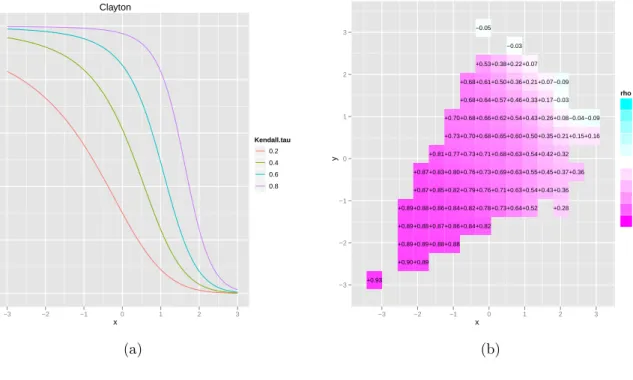
Example 3.1 (Clayton copula). The Clayton copula is an asymmetric copula, exhibiting
greater dependence in the negative tail than in the positive (i.e. lower tail dependence). The
generator for the Clayton copula is ϕ(t) = 1
θ(t
thus be written as CθCl(u1, u2) = (u−1θ+u −θ 2 −1) −1/θ, with derivatives C1(u1, u2) = 1 +uθ1(u−2θ−1)− θ+1 θ C11(u1, u2) = (θ+ 1)uθ2−1(1−u −θ 2 )(1 +u θ 1(u −θ 2 −1)) −1/θ−2
Since C11(q, q) = (θ+ 1)q−1(1−qθ)(2−qθ)−1/θ−2 → 0 as q →1− we have that ρ(s, s) →0
as s→ ∞. On the other hand, it can be shown that −C11(q, q)φ(Φ−1(q))→ ∞ as q→ 0+
so that ρ(s, s)→ 1 as s→ −∞. These features can be seen in figure 1. These plots give a
directly interpretable local dependence structure in terms of local correlation.
Figure 1: Local gaussian correlation for the clayton copula: (a) along the diagonal x1 =x2;
(b) estimated based on n= 500 observations.
Clayton x LGC 0.0 0.2 0.4 0.6 0.8 1.0 −3 −2 −1 0 1 2 3 Kendall.tau 0.2 0.4 0.6 0.8 (a) x y −3 −2 −1 0 1 2 3 +0.93 +0.90+0.89 +0.89+0.89+0.88+0.88 +0.89+0.88+0.87+0.86+0.84+0.82 +0.89+0.88+0.86+0.84+0.82+0.78+0.73+0.64+0.52 +0.28 +0.87+0.85+0.82+0.79+0.76+0.71+0.63+0.54+0.43+0.36 +0.87+0.83+0.80+0.76+0.73+0.69+0.63+0.55+0.45+0.37+0.36 +0.81+0.77+0.73+0.71+0.68+0.63+0.54+0.42+0.32 +0.73+0.70+0.68+0.65+0.60+0.50+0.35+0.21+0.15+0.16 +0.70+0.68+0.66+0.62+0.54+0.43+0.26+0.08−0.04−0.09 +0.68+0.64+0.57+0.46+0.33+0.17−0.03 +0.68+0.61+0.50+0.36+0.21+0.07−0.09 +0.53+0.38+0.22+0.07 −0.03 −0.05 −3 −2 −1 0 1 2 3 rho −1.0 −0.8 −0.6 −0.4 −0.2 0.0 0.2 0.4 0.6 0.8 1.0 (b)
Example 3.2 (Gumbel copula). The Gumbel copula is also an asymmetric copula,
Its generator function is ϕ(t) = (−lnt)θ for θ ≥1, thus the Gumbel copula can be written as CθGu(u1, u2) = exp h −((−lnu1)θ+ (−lnu2)θ)1/θ i .
The functions C1 and C11 are quite complicated and are therefore not given here. The
characteristics of ρ(x1, x2) for the Gumbel copula can be seen in figure 2 where we clearly
see the upper tail dependence numerically quantified in terms of the local correlation.
Figure 2: Local gaussian correlation for the gumbel copula: (a) along the diagonal x1 =x2;
(b) estimated based on n= 500 observations.
Gumbel x LGC 0.0 0.2 0.4 0.6 0.8 1.0 −3 −2 −1 0 1 2 3 Kendall.tau 0.2 0.4 0.6 0.8 (a) x y −2 −1 0 1 2 +0.50 +0.36 +0.45 +0.50 +0.47 +0.23 +0.34 +0.42 +0.45 +0.46 +0.43 +0.39 +0.36 +0.42 +0.44 +0.44 +0.42 +0.40 +0.38 +0.24 +0.31 +0.39 +0.44 +0.46 +0.46 +0.45 +0.43 +0.42 +0.43 +0.45 +0.29 +0.35 +0.43 +0.48 +0.50 +0.50 +0.49 +0.48 +0.49 +0.51 +0.55 +0.39 +0.46 +0.51 +0.54 +0.55 +0.55 +0.55 +0.56 +0.58 +0.62 +0.35 +0.42 +0.48 +0.53 +0.56 +0.58 +0.59 +0.60 +0.61 +0.63 +0.66 +0.39 +0.45 +0.50 +0.54 +0.57 +0.61 +0.63 +0.64 +0.65 +0.66 +0.67 +0.68 +0.52 +0.56 +0.61 +0.65 +0.67 +0.68 +0.68 +0.68 +0.69 +0.47 +0.52 +0.59 +0.65 +0.68 +0.69 +0.70 +0.71 +0.72 +0.39 +0.54 +0.64 +0.69 +0.71 +0.72 +0.74 +0.76 +0.77 +0.70 +0.74 +0.76 +0.78 +0.80 +0.81 +0.82 +0.83 +0.84 +0.86 +0.85 −2 −1 0 1 2 rho −1.0 −0.8 −0.6 −0.4 −0.2 0.0 0.2 0.4 0.6 0.8 1.0 (b)
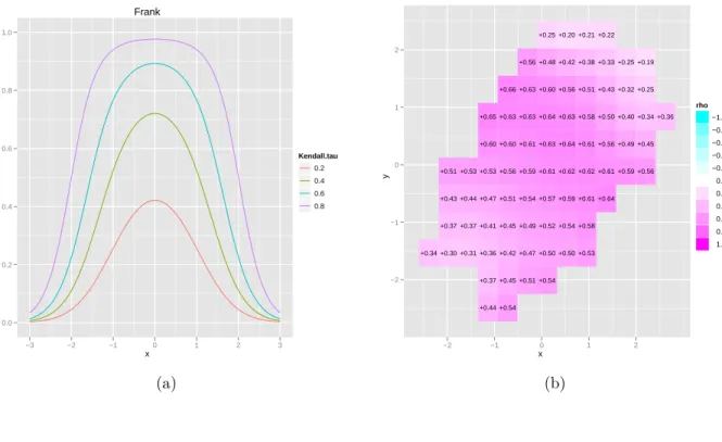
Example 3.3 (Frank copula). Define qz =e−θz−1. The generator for the Frank copula is
ϕ(t) =−ln(qt/q1). Then the Frank copula may be written as
The derivativesC1 and C1 are C1(u1, u2) = qu1qu2+qu2 qu1qu2 +q1 C11(u1, u2) = qu01qu2(q1−qu2) (qu1qu2 +q1) 2
It is easily seen that C11(q, q) → 0 when q → 0+ and when q → 1−. Thus the ρ(x1, x2)
goes to zero in both the upper and lower tail. This feature is reflected in figure 3; close to constant dependence in the center which vanish in the tails.
Figure 3: Local gaussian correlation for the gumbel copula: (a) along the diagonal x1 =x2;
(b) estimated based on n= 500 observations.
Frank x LGC 0.0 0.2 0.4 0.6 0.8 1.0 −3 −2 −1 0 1 2 3 Kendall.tau 0.2 0.4 0.6 0.8 (a) x y −2 −1 0 1 2 +0.44 +0.54 +0.37 +0.45 +0.51 +0.54 +0.34 +0.30 +0.31 +0.36 +0.42 +0.47 +0.50 +0.50 +0.53 +0.37 +0.37 +0.41 +0.45 +0.49 +0.52 +0.54 +0.58 +0.43 +0.44 +0.47 +0.51 +0.54 +0.57 +0.59 +0.61 +0.64 +0.51 +0.53 +0.53 +0.56 +0.59 +0.61 +0.62 +0.62 +0.61 +0.59 +0.56 +0.60 +0.60 +0.61 +0.63 +0.64 +0.61 +0.56 +0.49 +0.45 +0.65 +0.63 +0.63 +0.64 +0.63 +0.58 +0.50 +0.40 +0.34 +0.36 +0.66 +0.63 +0.60 +0.56 +0.51 +0.43 +0.32 +0.25 +0.56 +0.48 +0.42 +0.38 +0.33 +0.25 +0.19 +0.25 +0.20 +0.21 +0.22 −2 −1 0 1 2 rho −1.0 −0.8 −0.6 −0.4 −0.2 0.0 0.2 0.4 0.6 0.8 1.0 (b) 3.1.2 Elliptical copulas
Elliptical copulas are simply the copulas of elliptical distributions. The key advantage of elliptical copula is that one can specify different levels of correlation between the marginals,
but a disadvantage is that elliptical copulas typically do not have closed form expressions. The most commonly used elliptical distributions are the Gaussian and Student-t distribu-tions.
Example 3.4 (Gaussian copula). For a given correlation matrix Σ =
1 ρ ρ 1 the Gaussian
copula with correlation matrix Σ can be written as
CΣGauss(u1, u2) = ΦΣ(Φ−1(u1),Φ−1(u2)) (3.19)
where ΦΣ is the joint bivariate distribution function of a Gaussian variable with mean vector
zero and correlation matrix Σ. In general, when (X1, X2) is Gaussian with mean vector zero
and correlation matrix Σ, thenX1|X2 =x2 ∼N(ρx2,1−ρ2). It follows that for the Gaussian
copula C1(u1, u2) = P(U2 ≤u2|U1 =u1) = P(Φ−1(U2)≤Φ−1(u2)|Φ−1(U1) = Φ−1(u1)) = Φ Φ −1(u 2)−ρΦ−1(u1) √ 1−ρ2 ! LettingR = Φ−1(u√2)−ρΦ−1(u1)
1−ρ2 and differentiating this expression once more with respect tou1
we get C11(u1, u2) = −ρ √ 1−ρ2φ(Φ−1(u 1)) φ(R)
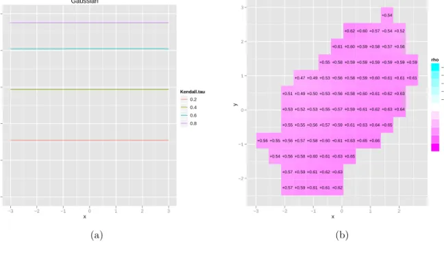
Thus for a Gaussian copula modelCGauss(F1(x1), F2(x2)) with arbitrary marginsF1 and F2,
ρ(x1, x2) is ρ(x1, x2) = −C11(F1(x1), F2(x2))φ(Φ−1(F1(x1))) q φ2(Φ−1(C 1(F1(x1), F2(x2)))) +C112 (F1(x1), F2(x2))φ2(Φ−1(F1(x1))) = φ(R)√ρ 1−ρ2 φ(Φ−1(F 1(x1))) φ(Φ−1(F 1(x1))) r φ(R)2+φ2(R) ρ2 1−ρ2 φ2(Φ−1(F 1(x1))) φ2(Φ−1(F 1(x1))) = √ ρ 1−ρ2+ρ2 =ρ (3.20)
This is of course valid for all (x1, x2), not only on a curve F1(x1) = F2(x2), and it shows
that a constant local Gaussian correlation is a feature of the Gaussian copula rather than the bivariate Gaussian distribution. Note that the local mean and local variance are not in
general constant for non-Gaussian marginals. For a non-Gaussian copula, ρ(x1, x2) will in
general depend on the margins. It remains to prove the converse statement that ρ(x) = c,
(−1 < c < 1, c 6= 0) implies the Gaussian copula. We do not know of any other than the Gaussian that has this property.
Figure 4: Local gaussian correlation for the gaussian copula: (a) along the diagonalx1 =x2;
(b) estimated based on n= 500 observations (where the copula parameter is ρ= 0.5877).
Gaussian x LGC 0.0 0.2 0.4 0.6 0.8 1.0 −3 −2 −1 0 1 2 3 Kendall.tau 0.2 0.4 0.6 0.8 (a) x y −2 −1 0 1 2 3 +0.57 +0.59 +0.61 +0.61 +0.62 +0.57 +0.59 +0.61 +0.62 +0.63 +0.54 +0.56 +0.58 +0.60 +0.61 +0.63 +0.65 +0.56 +0.55 +0.56 +0.57 +0.58 +0.60 +0.61 +0.63 +0.65 +0.66 +0.55 +0.55 +0.56 +0.57 +0.59 +0.61 +0.63 +0.64 +0.65 +0.53 +0.52 +0.53 +0.55 +0.57 +0.59 +0.61 +0.62 +0.63 +0.64 +0.51 +0.49 +0.50 +0.53 +0.56 +0.58 +0.60 +0.61 +0.62 +0.63 +0.47 +0.49 +0.53 +0.56 +0.58 +0.59 +0.60 +0.61 +0.61 +0.61 +0.55 +0.58 +0.59 +0.59 +0.59 +0.59 +0.59 +0.59 +0.61 +0.60 +0.59 +0.58 +0.57 +0.56 +0.62 +0.60 +0.57 +0.54 +0.52 +0.54 −3 −2 −1 0 1 2 rho −1.0 −0.8 −0.6 −0.4 −0.2 0.0 0.2 0.4 0.6 0.8 1.0 (b)
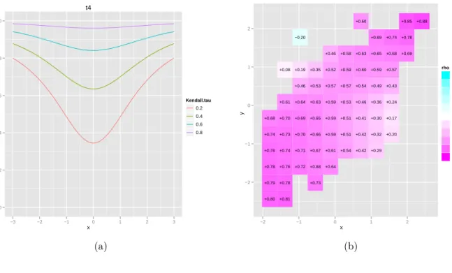
Example 3.5(T-copula).In the case that (X1, X2) is t-distributed withνdegrees of freedom
and correlation coefficient ρ, we have that X1|X2 = x2 is t-distributed with ν+ 1 degrees
of freedom, expected value ρx2 and variance
ν+x2 2
ν+1
(1−ρ2). With tν as the standard
t-distribution function, a similar argument as for the Gaussian copula leads to
C1(u1, u2) =tν+1 t−1 ν (u2)−ρt−ν1(u1) r (ν+t−1ν (u1)2)(1−ρ2) ν+1 :=tν+1(R),
and with ftv as the standard t-density function and b= r (ν+t−1ν (u1)2)(1−ρ2) ν+1 C11(u1, u2) = ∂R ∂u1 ftν+1(R) = −ftν+1(R) ftν(t −1 ν (u1))b2 ρb+ 1−ρ 2 ν+ 1t −1 ν (u1)R ! ,
No simple formula for ρ(x1, x2) comes as a result of this. In figure 5 a) we see that ρ(s, s)
increase towards each tail which is consistent with the t-copula having both upper and lower tail-dependence.
Figure 5: Local gaussian correlation for the student t-copula: (a) along the diagonalx1 =x2;
(b) Estimated based on n= 500 observations.
t4 x LGC 0.0 0.2 0.4 0.6 0.8 1.0 −3 −2 −1 0 1 2 3 Kendall.tau 0.2 0.4 0.6 0.8 (a) x y −2 −1 0 1 2 +0.80 +0.81 +0.79 +0.78 +0.73 +0.78 +0.76 +0.72 +0.68 +0.64 +0.76 +0.74 +0.71 +0.67 +0.61 +0.54 +0.42 +0.29 +0.74 +0.73 +0.70 +0.66 +0.59 +0.51 +0.42 +0.32 +0.20 +0.68 +0.70 +0.69 +0.65 +0.59 +0.51 +0.41 +0.30 +0.17 +0.61 +0.64 +0.63 +0.59 +0.53 +0.46 +0.36 +0.24 +0.46 +0.53 +0.57 +0.57 +0.54 +0.49 +0.43 +0.08 +0.19 +0.35 +0.52 +0.59 +0.60 +0.59 +0.57 +0.46 +0.58 +0.63 +0.65 +0.68 +0.69 −0.20 +0.69 +0.74 +0.78 +0.60 +0.85 +0.88 −2 −1 0 1 2 rho −1.0 −0.8 −0.6 −0.4 −0.2 0.0 0.2 0.4 0.6 0.8 1.0 (b)
Example 3.6. (Role of margins) It is of great interest to investigate how the choice of
mar-gins affects the local Gaussian correlation. For many combinations of marginal distributions
ρ(x1, x2) typically reveals the same pattern as long as the copula is kept fixed. In figure 6 we
have plotted ρ(x1, x2) along the diagonal for the t-copula (4 degrees of freedom, ρ = 0.58),
but with margins F1 = F2 = tv where tv is the t-distribution function with v degrees of
choice of margins only affects the speed at which ρ(s, s) goes to 1 in the tails. This is quite
clear since the degrees of freedom determines the rate at which tv(x) → 0,1 as x → ±∞,
which in turn influences the rate at which the numerator of (3.2) goes to ∞.
Figure 6: ρ(x1, x2) for the t-copula with 4 degrees of freedom andρ= 0.587 (τ = 0.4). Both
margins are t-distributed with v degrees of freedom, v = 1,4,8,100.
t4 x LGC 0.6 0.7 0.8 0.9 1.0 −3 −2 −1 0 1 2 3 df 1 4 8 100
4
Evaluating copula models
Given iid observations X1, . . . , Xn from F(x1, x2) = C(F1(x1), F2(x1)) consider the issue of
using local Gaussian correlation to test the null hypothesis
H0 :C∈ C, C ={Cθ :θ∈Θ}, (4.1)
where Θ is the parameter space. Let ρθ(·) denote the local Gaussian correlation of the
distribution functionCθ(F1(x1), F2(x1)) (given by (3.9)). A natural approach is to compare
the functionρθ(·) estimated under H0 with the nonparametric estimate described in section
replacing θ, F1 and F2 in the analytical expression (3.9) with corresponding estimates under
H0.
4.1
Parametric estimation of local Gaussian correlation
Sinceρθ(·) depends on the marginsF1 andF2 we would, for a full parametric approach, need
to make the additional parametric assumption that
H00 :F1 ∈ F1, F2 ∈ F2,
and thus restricting ourselves to the more narrow null hypothesis H0 ∩H
0
0. This problem
may be overcome by estimating Fj by the empirical distribution function
ˆ Fj(x) = 1 n n X i=1 1(Xij ≤x), j = 1,2. (4.2)
The same issue is also encountered when estimating the copula parameter θ under H0,
where a full maximum likelihood approach or the ”Inference Functions for Margins” (IMF)
approach [see Joe, 1997] requires the additional assumption H00. This assumption can be
avoided by replacing Fj in the likelihood by the empirical distribution function ˆFj(x) (4.2).
This method is denoted the pseudo-likelihood [Demarta and McNeil, 2005] or the canonical maximum likelihood [Romano, 2002]. To avoid that the copula density blows up at the
boundary of [0,1]2 one typically base the pseudo-likelihood estimation on the scaled ranks
U1 = (U11, U12). . . , Un = (Un1, Un2) whereUij =nFˆj(Xij)/(n+1). These values are called the
pseudo-observations, and given independent observations X1, ..., Xn from C(F1(x1), F2(x1))
they can be interpreted as a sample from the underlying copula C. However, one should
note that the observations are not mutually independent. By using the pseudo-observations one could also estimate the copula parameter using the relation to Kendall-s tau given by equation (3.14). For other rank-based estimators see Tsukahara [2005] and Chen et al. [2006].
Let θn = θn(U1, . . . , Un) denote an estimate of the copula parameter under H0 based
on the pseudo observations (U1, . . . , Un). Then a plug-in estimator ρθn(·) of ρθ(·) is given
by (3.9) with θ replaced by θn and with the marginal distribution functions Fj replaced by
ˆ
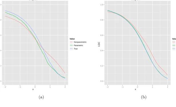
described in section 2. In general, ρθn(·) will converge considerably faster towardsρθ(·) than
ρn,b(·) since it is based on ˆFj and θn which has the ordinary parametric convergence rate,
whereas (Tjøstheim and Hufthammer [2012]) ρn,b(·) has a substantially slower rate. Figure
7 displays the estimates ρθn(·) and ρn,b(·) along the diagonal when F1 and F2 are standard
gaussian and C is the Clayton copula. In figure 7 (a) the estimates are based on n = 500
observations and in figure 7 (b) n = 5000. Note that ρn,b(·) is biased. This bias can be
adjusted for, but this problem will be studied generally in a separate publication.
Figure 7: Plot of the true local Gaussian correlationρθ(s, s), the parametric estimateρθn(s, s)
and the nonparametric estimate ρn,b(s, s) against s for the Clayton copula with standard
normal margins: (a) n = 500,b1 =b2 = 1; (b)n = 5000,b1 =b2 = 0.5
Clayton x LGC 0.0 0.2 0.4 0.6 0.8 1.0 −2 −1 0 1 2 Value Nonparametric Parametric True (a) Clayton x LGC 0.0 0.2 0.4 0.6 0.8 1.0 −2 −1 0 1 2 Value Nonparametric Parametric True (b)
4.2
A bootstrap based Goodness-of-fit test
We now turn to the problem of constructing a goodness-of-fit test forH0. Having established
goodness-of-fit test on the process
Pn(·) =ρn,b(·)−ρθn(·), (4.3)
where ρn,b(·) is the estimate obtained by using the local likelihood method described in
section 2. Aggregation of Pn2 onR2 is done over a prespecified grid (x1, . . . , xp) by
Tn= p
X
i=1
Pn(xi)2, (4.4)
where large values of Tn lead to the rejection of H0. By the construction of Tn it is clear
that its asymptotic distribution (when scaled properly by some function δ(n, b)) in general
depends on the underlying copula and the parameter θ, which in turns means that critical
values can not be tabulated by means of the asymptotic properties. Moreover, it is known (see e.g. Terasvirta et al. [2010] chapter 7.7) that in general the asymptotics of functional
tests like Tn are not very accurate. We therefore use a parametric bootstrap similar to that
of Genest et al. [2009] (see also Stute et al. [1993]) to obtain approximate P-values. The parametric bootstrap procedure is as follows:
Parametric bootstrap
1. Estimate θ, F1 and F2 byθn =θn(U1, . . . , Un), ˆF1 and ˆF2.
2. Obtain ρn,b(·) by the local likelihood method and ρθn(·) by replacing θ, F1 and F2 in
(3.9) by θn, ˆF1 and ˆF2. Compute the value ofTn.
3. For some large integer R, repeat the following steps for everyk ∈ {1, . . . , R}:
(a) Generate a random sample X1∗k, . . . , Xnk∗ from the distribution
F∗(x) = Cθn( ˆF1(x1),Fˆ2(x2)).
(b) Compute Tn,k∗ by repeating step 1 and 2 for this sample.
The P-value for this test can then be approximated by R−1PR
k=11(T
∗
n,k > Tn).
we have chosen to estimate θ by θn = m−1(ˆτ) where ˆτ is the sample Kendall’s tau and
m is defined by 3.14. The margins F1 and F2 are typically estimated by their empirical
counterpart given by (4.2), but for n small we suggest using smoothed nonparametric
estimates.
Remember that the local likelihood estimate ρn,b(·) is only consistent with the
ana-lytical expression (3.9) along the curve F1(x1) = F2(x2). This means that each gridpoint
xi = (xi1, xi2), i = 1, . . . p should be chosen so that ˆF1(xi1) ≈ Fˆ2(xi2). For example, given
suitable values xi1, i = 1, . . . , p one can take xi2 = ˆF2−1( ˆF1(xi1)), where ˆFj is given by
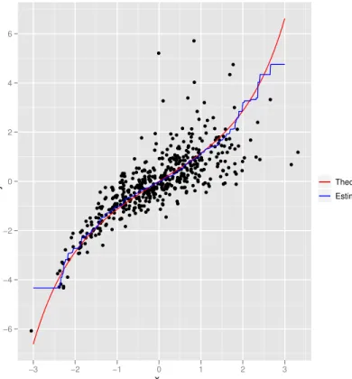
(4.2). Such a curve is illustrated in figure 8. However, this is somewhat restrictive and we therefore provide a second bootstrap procedure which does not rely on the analytical
expression (3.9) but where we instead estimate ρθ by monte carlo approximation:
Double parametric bootstrap
1. Estimate θ, F1 and F2 byθn =θn(U1, . . . , Un), ˆF1 and ˆF2.
2. Obtainρn,b(·) by the local likelihood method andρθn(·) by monte carlo approximation:
(a) For some (preferable large) integer m ≥ n generate a random samle V1∗, . . . , Vm∗
from the distributionF∗(x) =Cθn( ˆFX1(x1),FˆX2(x2)).
(b) Approximate ρθn(·) by ρn,b(·) based on V
∗
1, . . . , V
∗ m.
(c) Compute the corresponding value of Tn.
3. For some large integer R, repeat the following steps for everyk ∈ {1, . . . , R}:
(a) Generate a random samle X1∗k, . . . , Xnk∗ from the distribution
F∗(x) = Cθn( ˆF1(x1),Fˆ2(x2)).
(b) Compute Tn,k∗ by repeating step 1 and 2 for this sample.
The P-value for this test can then be approximated by R−1PR
k=11(T
∗
n,k > Tn).
In Genest et al. [2009] a similar bootstrap procedure is used for a number of test statistics in the context of copula goodness-of-fit testing. There it is concluded that for the
Figure 8: Plot of the curves x2 =F2−1(F1(x1)) and x2 = ˆF2−1( ˆF1(x1)) when the data comes
fromCθ(φ(x1), t4(x2)), whereCθ is the Clayton copula with θ = 3, φis the standard normal
distribution function andt4 is the Student’s t-distribution function with 4 degrees of freedom.
x y −6 −4 −2 0 2 4 6 −3 −2 −1 0 1 2 3 Theoretical Estimated
than the sample size n (minimumm= 2500 when n= 150). In our case we can expect that
even larger values of m is required since a larger m is balanced out by a smaller bandwidth
b. This makes the double-boostrap computational demanding and, consequently, we only
considered the one-level parametric bootstrap in the simulation study in section 4.4. The
advantage of this boostrap procedure is that we can choose the grid (x1, . . . , xp) freely and
that it can be used whenever the analytical expression (3.9) is not available. The selection of gridpoints can be done as in Jones and Koch [2003] and Berentsen and Tjøstheim [2012]: First place a regular grid over the area of interest and then select the gridpoints satisfying
ˆ
f(xi) > C for some constant C and a density estimator ˆf. Alternatively, if the user is
interested in a good fit in a particular region the grid can be specified manually, for example in the context of risk management where the fit of the tails are specially important.
4.3
Choice of bandwidth
Choosing the correct bandwidth for the estimateρn,b is in general a difficult task and an
im-portant topic for future research. A practical bandwidth algorithm is proposed by Tjøstheim
and Hufthammer [2012], but when testing H0 : C ∈ C we may choose the bandwidth such
that it is optimal if H0 is true. In general, when the distribution function of X is given by
F(x) =Cθ(F1(x1), F2(x2)) the mean sum of squared error over a grid (x1, . . . , xp) is given by
MSSE(ρn,b(·)) =E p X i=1 (ρn,b(xi)−ρθ(xi)) 2 ! (4.5)
Since ρθn(·) converges faster than ρn,b(·) (under H0) it is reasonable to choose b as the
minimizer of \ MSSE(ρn,b(·)) =E∗ n X i=1 (ρn,b(xi)−ρθn(xi)) 2 ! (4.6)
where the expectation E∗ is with respect to the distribution function F∗(x) =
Cθn( ˆF1(x1),Fˆ2(x2)) estimated underH0. If the grid is the same as for the test statisticTn, this
amounts to minimising the bootstrap mean of the statistic Tn, i.e. MSSE(\ ρn,b(·)) = E∗(Tn).
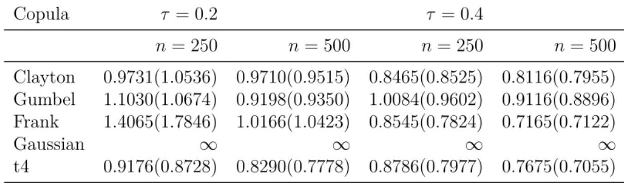
Table 1 reports bandwidth estimates based on minimizing (4.6). For simplicity b1 =
b2 =b. The resampling distribution F∗(x) =Cθn( ˆF1(x1),Fˆ2(x2)) is calculated from a single
and τ = 0.2,0.4. Standard normal margins where used, i.e. F1 =F2 = Φ. For comparison,
the minimiser of (4.5) (which is computed by monte carlo integration) is given in parentheses.
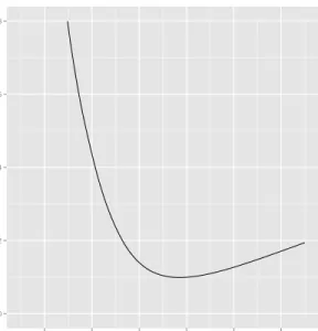
Figure 9 displays MSSE(\ ρn,b(·)) as a function of b when C is the Clayton copula.
Not supricingly, neither (4.5) nor (4.6) has a minimum for the Gaussian copula (both
decrease as b increases). This is a result of the local Gaussian likelihood beeing equivalent
with the global Gaussian likelihood when b → ∞. However, it is not recommended to use
a very large bandwidth when testing for the Gaussian copula, since too much smoothing results in poor power when the null hypothesis is false.
Figure 9: MSSE(\ ρn,b(·)) versusb for the Clayton copula.
h MSSE 0.0 0.2 0.4 0.6 0.8 0.4 0.6 0.8 1.0 1.2 1.4
Table 1: Estimated bandwidth based on MSSE(\ ρn,b(·)) calculated from a single sample from
each copula model for n = 250,500 and τ = 0.2,0.4. The minimizer of MSSE(ρn,b(·)) is
given in the parentheses.
Copula τ = 0.2 τ = 0.4 n = 250 n = 500 n= 250 n= 500 Clayton 0.9731(1.0536) 0.9710(0.9515) 0.8465(0.8525) 0.8116(0.7955) Gumbel 1.1030(1.0674) 0.9198(0.9350) 1.0084(0.9602) 0.9116(0.8896) Frank 1.4065(1.7846) 1.0166(1.0423) 0.8545(0.7824) 0.7165(0.7122) Gaussian ∞ ∞ ∞ ∞ t4 0.9176(0.8728) 0.8290(0.7778) 0.8786(0.7977) 0.7675(0.7055)
4.4
Simulation study
A Monte Carlo study is performed to assess the finite-sample properties of the proposed goodness-of-fit test (4.4) (based on the one-level parametric bootstrap). In order to examine
its performance, we compare it with a much used test proposed by Genest and R´emillard
[2008].
This particular test is chosen because of its good overall performance in the simulation studies of Genest et al. [2009] and Berg [2009]. The test is based on the empirical copula process Cn(u) = 1 n n X i=1 1(Ui1 ≤u1, Ui2 ≤u2), (4.7)
where Ui = (Ui1, Ui2) i = 1, . . . , n are the pseudo-observations and u = (u1, u2) ∈[0,1]2. A
natural test consist in comparing a distance between Cn and an estimateCθn of C obtained
under H0. Then a goodness-of-fit test may be based on the Cramer-von-Mise type statistic
An=n
Z
[0,1]2{Cn(u)−Cθn(u)}
2dC
n(u), (4.8)
which in turn may be estimated by ˆAn = Pni=1{Cn(Ui)−Cθn(Ui)}
2. Further one proceed
by parametric bootstrap analogue to the first procedure described in section 4.2 to find an
approximate P-value for the test. If an analytical expression for Cθ is not available one
may resort to a double parametric bootstrap analogue to the second bootstrap procedure described in section 4.2. For a more detailed description of these test procedures we refer to