On particle filter localization and mapping for Nao robot

(1)

ON PARTICLE FILTER LOCALIZATION AND MAPPING FOR NAO

ROBOT

Master of Science thesis

Examiner: prof. Risto Ritala

Examiner and topic approved by the Faculty Council of the Faculty of Engineering Sciences

(2)

ABSTRACT

ANDREAS UWAOMA: On particle filter localization and mapping for Nao robot. Tampere University of Technology

Master of Science Thesis, 58 pages, 20 Appendix pages June 2015

Master’s Degree Program in Machine Automation Major: Mechatronics and Micromachines

Examiner: Professor Risto Ritala

Keywords: Humanoid robot, Nao, Localization, Particle filters, Path planning.

The performance of autonomous mobile robots within an indoor environment relies on an effective detection and localization system. Self-Localization within an indoor environment has been studied and tested experimentally on humanoid robot Nao. The solution utilizes a pre-existing map with known and unknown features.

The aim of this thesis is to utilize map of visual features and the Monte-Carlo Scheme (particle filters) in localization and navigation. Nao robot cameras has been used for detection Naomarks, the detection of these features provides an estimation of the relative distances of features to current robot position. These measurements are applied to a visual localization algorithm that uses a pair of known feature to localize the robot, furthermore the measurements is fused to a particle filter algorithm for estimating the pose of the robot within the map. The particle filter implementation was based on the C++ programming language. A simple path planning scheme was implemented for continuous localization while navigating a paths with obstacles.

The algorithms has been tested with reference to measurements provided by an external sensor. The results of the implementations indicates that the robot can effectively navigate from a start position to a predefined location while avoiding obstacles on its path.

(3)

PREFACE

This thesis work has been realized at the department of Automation Science and Engineering with the help of a number of people, whom I would like to thank.

First, special thanks to my supervisor, Professor Risto Ritala for providing the resources and the much needed guidance through this thesis.

I also like to thank Mikko Lauri, Joonas Melin and everyone who provided technical support and suggestions through the implementation of this work.

Lastly, express my gratitude to my family for their love and encouragement through the challenging times of my studies.

Tampere, 30.06.2015 Uwaoma Andreas E.

(4)

LIST OF FIGURES

Figure 2.1. Robo-tuna biomimetic robot...5

Figure 2.3. Pose data comparison; augmented MCL, top camera localization and odometry data...9

Figure 2.2. A typical Kalman filter application...10

Figure 3.1. The Nao robot...14

Figure 3.2. Nao sensors and joints...15

Figure 3.3. Head tactile sensors: A: front, B: middle, and C: rear sensors...16

Figure 3.4. Nao’s cameras field of view...17

Figure 3.5. Nao Software Interaction...19

Figure 3.6. Naoqi Framework...20

Figure 3.7. Screenshot of the Choregraphe software...24

Figure 4.1. Walk path of Nao robot for 200cm command along x-axis...28

Figure 4.2. Naomarks samples...29

Figure 4.3. Naomark dimension ...31

Figure 4.4. Nao Camera angles ...32

Figure 4.5. Nao Frame and global frame ...34

Figure 4.6. Representation of marker locations in global and robot frame ...35

Figure 4.7. Illustration of robot and with a specified target coordinate ...42

Figure 4.8. Flow-chart of the navigation and localization program ...44

Figure 4.9. Class Structure of the implementation ...45

Figure 5.1. Distance and lateral displacement for 200 cm straight walk ...46

Figure 5.2. Distance and lateral displacement for 100 cm straight walk ...47

Figure 5.3. Visual localization result ...48

Figure 5.4. Particle pose estimate after move [0.8, 300_{] ...50}

Figure 5.5. Particle pose estimate for target coordinates [1.3, 1.0] ...52

Figure 5.6. Particle pose estimate for target coordinates [0.5, 0.6]...53

Figure 5.7. Particle pose estimate for (a) an obstacle at [0.6, 0.6]...54

Figure 5.8. Estimate of robot position (b) obstacle at [0.6 0.6] evaded ...55

Figure 5.9. Estimate of robot position at (c) final target coordinates [1.3, 1.2]...56

(7)

LIST OF TABLES

Table 4.1. Walk measurements. ...26 Table 4.2. Robot turn measurements for angles 180, 90 and 45 degrees. ...27 Table 4.3. Global coordinate of markers on map. ...33 Table 5.1. Localization experiment using known start points, distance and direction

Command. ...49 Table 5.2. Localization experiment using known start points and target coordinates..51 Table 5.3. Results of autonomous localization with obstacles. ...56

(8)

1 INTRODUCTION

The Intelligent Sensing Laboratory of Automation Science and Engineering (ASE) aims at developing methods for autonomous mobile robots to interact and navigate within a specified environment. The long-term goal of the research in intelligent sensing is to develop processes whereby the robots can focus their attention so that they optimally perform task such as autonomous navigation, obstacle detection and avoidance and social interaction. Over the years, research and development of mobile robots has produced promising results with the advent of Honda’s ASIMO and Sony’s AIBO. Recently a new platform Nao developed by Aldebaran robotics has become very popular amongst researchers. Nao platform has gained a lot of interest due to its relatively low-cost, array of available sensors and relative ease of programming.

A common task for a mobile robot is to follow an object at a specific distance while simultaneously localizing itself in the environment. In order to perform this function, the robot must be able recognize the object and also identify specific features in the environment. Using the detected features the robot should be able to guide itself towards a specified target while avoiding bumping into obstacles on its path.

1.1 Objective

The objective of this thesis is to implement a particle filter based solution for localization and mapping of mobile robot provided by the Nao platform. The work is divided into the following tasks:

· Create map of known environment based on features. · Implement self-localization on Nao using monocular vision.

· Implement a sequential Monte-Carlo scheme to verify the performance of the localization algorithm.

The self-localization on Nao robot involves definition of the map based on features that can be easily identified by the robot. Applying a set of actions that is required for the robot to reach a set goal point within the map and determining the robot’s pose at each state by matching actions and new observations to previous states.

(9)

1.2 Contribution

The major contributions to this thesis can be summarized as follows:

· A sequential Monte-Carlo Scheme (SMC) is implemented for Nao localization based on C++ programming language.

· A feature based map is developed using Nao markers for an environment with incomplete information about obstacles.

· Visual localization is implemented using information from the map.

The implementation of SMC undertaken in this thesis is a verification of the Nao robot’s capabilities in the C++ programming environment. This implementation can be further explored within capabilities of the platform for a more robust scheme for tasks such as path planning etc.

1.3 Thesis structure

The structure of the thesis is as follows;

Chapter 2 contains an overview of mobile robots, and a brief timeline of developments in mobile robotics. The chapter also discusses the main ideas in mobile robotics. Key concepts, such as navigation, path planning, active sensing, vision and localization are briefly explained. In addition previous works based on biped robots are presented.

Chapter 3 introduces the robotic platform Nao. The hardware and software will be described in detail. The chapter also describes the sensors available on the platform, the mode of operation of the sensors, actuators and the available programming methods. The rest of the chapter will be focused on a thorough examination of modules pertinent to the thesis.

Chapter 4 describes the methods used in the implementation. The SMC, the visual localization and the Nao visual sensing information obtained from features will be covered here. Furthermore, the chapter presents the approach to programming, challenges encountered during implementation, an analysis of the decision taken during the implementation and the factors that necessitated such decisions.

(10)

Chapter 5 presents the results of the implementation. The chapter discusses the result of the SMC and visual localization.

A summary of the works completed is presented in Chapter 6. Suggestion on future works based on the experience gained from this thesis and the uses of the platform is presented.

(11)

2

REVIEW OF MOBILE ROBOTICS

Operation of an autonomous mobile robot in complex locations such as factory floors, homes or generally within maze-like environment requires a dependable 'self-localization' system. This section will present a general overview of autonomous mobile robots, past development in mobile robotics and an explanation of key concepts such as autonomous navigation, path planning, obstacle avoidance and sensing. The rest of the section will review the earlier works based on the biped robot platforms.

2.1 Autonomous mobile robots

Autonomous mobile robots have become an interesting discourse for several reasons. First, mobile robots are less viewed as mere computers on wheels having ability to detect some physical properties in their environment using inbuilt sensors. A mobile robot is an intelligent agent that combines a host of computers, actuators and an array of sensors whereby it is able to detect features, identify patterns and build a knowledge base of its operational environment. With this knowledge base, the robot is able to navigate, and perform required tasks in the learned environment and adapt the knowledge to environment not previously learned.

In earlier developments in mobile robots, robots were designed to mimic functions of humans and other species. One of such robots is Robotuna developed by David Barret [1] of MIT as part of his doctoral thesis in 1995. The robot is a biomimetic robot that moves through water by swimming like a biological fish. His design has been adopted and further developed by Boston engineering as a 4 foot long undersea vehicle that can blend with marine life and perform both civilian and military missions. Honda’s “Prototype model 2” humanoid robot that was first shown in 1996 had the ability to stand like a human. The most progress came with Sony’s robotic dog Aibo introduced in 1999 and Honda’s Humanoid robot Asimo introduced a year after. Both platforms had the ability to walk, run, communicate with humans and interact with the environment.

(12)

Figure 2.1 Robo-tuna developed by Boston engineering [14]

Autonomous robots has since developed into various types of land based robots, underwater robot, and aerial robots. Each of these having characteristics that best suits their operational environment.

2.2 Autonomous navigation

Navigation is “the process of accurately [2] determining position and velocity relative to a known reference”. It is a goal orientated behavior that moves an agent between its present location and the desired location. Autonomous navigation is when the agent exhibits this behavior with little or no human intervention.

Autonomous navigation is one of the most challenging competences required of a mobile robot. For a robot to successfully navigate an environment, the robot must be capable of the following key functions.

· Perception · Cognition · Localization · Motion control.

Perception requires that the robot is able to extract useful data about its environment using an array of sensors. The data extracted is processed by the onboard computers and the robot is able to make decision based on the data.

(13)

Cognition requires that the robot can decide on how to achieve its goals. The robot must be able to decide the specific actions from a set of possible actions that will take it from its present state to the goals.

Localization requires that the robot is able to determine its own location with respect to some external reference. The challenge here is to actively combine data from sensors such as cameras and time of flight sensors with the odometry data such that the mobile robot becomes aware of its state in the environment. Identifying its absolute location locally or globally is not enough for localization. Determining its relative position to humans, objects or other robot that might be operating in same space is equally important for the appropriate performance of task.

Motion control requires that the robot can regulate its actuators’ output in order to attain the desired motion trajectory.

Amongst the four critical functions described, extensive attention has been devoted to localization and this has produced several new and evolving approaches to how autonomous mobile robots operate. Some of the approaches will be discussed in subsequent sections of this chapter.

2.3 Path planning and obstacle avoidance

Path planning, also referred to as motion planning, involves finding a sequence of actions that transforms an agent from an initial state to the desired goal state. In path planning, the states represent the location of the agents while the actions the agent can take, each having an associated cost attached is the transition. The path is optimal if the sum of associated transition costs across the possible paths leading from the initial location to the goal position is minimized. When planning paths, for example the completeness of the path and the optimality of the path need to be considered.

A path planning algorithm iscomplete if the agent is guaranteed to find a path in a finite time when one exists and will let us know if no path exists. Similarly, the planning algorithm isoptimal if it is guaranteed to find the optimal path.

In mobile robotics, topological path planning consists of representing the environment of the robot as a graph with nodes and edges. The cost of each edge represents the cost

(14)

of transiting between two nodes. Path planning can then be treated as a simple search of sequence of nodes that connects the start node to the desired end node at an admissible cost. A number of methods have been developed for computing least cost path. Two common methods are Dijkstra’s algorithm (Dijkstra 1959) and the A*(Hart, Nelson & Rafael 1968).

Obstacle avoidance is a key factor for the successful operation of an autonomous mobile robot. Virtually all mobile robots feature some form of collision avoidance ranging from primitive algorithms to well-developed algorithms that manage detection using sensors and stop the robot short of an obstacle or enables the robot to detour around the obstacle to avoid collision.

Common obstacle avoidance methods include edge detection, occupancy grids and virtual force fields (VFF) [3-4].

In the edge detection method, the avoidance algorithm attempts to determine the position of vertical edges and consequently steers around the detected edge. The lines connecting detected edges are considered as obstacle boundaries. The edge detection method though popular, has several limitations. The efficacy of this method depends on the sensitivity and accuracy of the sensors. In the case of sonar sensors which are commonly used in mobile robotics, there are many shortcomings, some of which are explained as follows.

The poor directionality limits the ability to detect the spatial position of the obstacle in ranges between 10cm - 40cm.

Specular reflections which occur when the angle of incidence between the wave front and a smooth surface is large, results in the surface reflecting the incoming ultrasonic beam away from the sensors. Furthermore, Ultrasonic noise form external sources often cause the robot to detect non exiting edges.

In the occupancy grid method, the robot’s work space is divided into small square cells of fixed sizes to form a grid. Each cell is assigned a certainty values that indicates the measure of confidence that an obstacle exists within that cell. The greater the certainty values the more likely the cell is occupied by an obstacle. As the robot moves within its work space while sampling continuously for obstacles, a stationary obstacle gives more count of echo readings while the incorrect readings are minimal due to randomness.

(15)

The virtual force field (VFF) method relies on the assumption that obstacles conceptually generate some potential field that repulses the robot as the robot approaches the obstacle. The closer the robot is to an obstacle the stronger the repulsive field.

The basic VFF method is a combination of the certainty grid described above with a potential field. While the mobile robot transverses the workspace, range readings are recorded and projected to a certainty grid. The algorithm scans small’s cells within the workspace that represents the possible locations of the robot. Each cell applies a repulsive force to the robot.

The magnitude of the repulsive field indicates the measure of certainty in the presence of an obstacle in the proximity of the cell. The magnitude of the certainty is inversely proportional to the square of the distance between the cell and the robot. The VFF method has a clear advantage over the edge detection method because incorrect readings are eliminated since VFF does not utilize sharp edges but responses to a cluster of densities. Furthermore, the grid representation allows the integration of data from different types of sensors for example vision, proximity and contact sensors.

2.4 Localization

2.4.1 Particle filter based localization

Particle filter based localization describes a probabilistic scheme that tracks a robot’s belief state using an arbitrary probability density function to represent the robot’s position. This scheme approximates a state and its variance by a set of samples – called particles - comprising possible states and weightings representing the probability of each state. The algorithm starts with a uniform random distribution over the configuration space, indicating the lack of information about robot’s initial location. Each point or position in the robot’s space is equally likely at this stage. When the position of the robot changes by a specified value, each particle is updated through the motion model. The update is performed according to the last control input to reflect the change in position of the robot. Weighting value is computed for each particle by considering the likelihood of data when observing specified landmarks. The particles are resampled with respect to their weights. Thus resampling is carried out such that particles which are consistent with sensor readings are more likely selected. After

(16)

several observations the particles converge to reflect a better estimate of the robots’ pose.

Predictive estimation of robot’s camera position and an implementation of the kinematic model based on the odometry system were proposed by Eshan Hashemi, et al [5]. Their work focused on the application of the Augmented Monte Carlo localization on the landmarks, lines, and points and optimized filtering parameters of robot state estimation. The current set of particles is obtained by an application of the motion model on the previous set according to the last control action issued to the robot. A weighting value is computed for each landmark by considering the observations of landmarks. The final weighting of particles is a numerical product of detect landmark probabilities.

Figure 2.2. Pose data comparison; augmented MCL (red pluses), top camera

localization [5] (blue lines), and odometry data (black lines)

In their implementation, the robot’s head was mounted with a colored outline to enable the tracking of poses and comparison with perceived positions and orientations. This tracking system utilizes an external Wi-Fi camera mounted above the work space. Independent tests were carried out on the robot for three different maneuvers both for simulated and empirical data. The result, see Fig. 2.2 shows ± 10 cm error in position and ± 5 degree error in orientation for the augmented MCL compared with the perceived position and orientation by the external reference camera.

(17)

2.4.2 Kalman filter based localization

The Kalman filter (KF) is a mathematical algorithm for estimating the state of a noisy linear dynamic system. The state refers to a vector of variables that describe the system. In the case of a mobile robot, the state vector is [x, y, Ө], where (x, y) is the coordinate of the location on a plane and theta is the orientation of the robot with respect to a reference. The KF produces an optimal estimate of a system’s state based on the knowledge of the system and measuring device, the description of the system noise and measurement errors and the uncertainty in the dynamics of the system.

Figure 2.3: A typical Kalman filter application [2]

The Kalman filter assumes that the system is linear, measurement noise and the model noise are independent, and all other noise in the system are white noise and can be modelled with a Gaussian distribution. Mobile robot localization commonly meets all these assumptions except that the trajectory of mobile robot is non-linear. This problem has been solved by a modification of the Kalman filter call extended Kalman filter (EKF). The EKF places the linear trajectory of the KF with an estimated trajectory that models the non-linearity of the system.

The Kalman filter is broken into two steps. The first is the prediction step or time update. At this step the state of the system is predicted based of the corresponding system kinematics. The second step is the correction or measurement update. During the

(18)

correction step, the state of the system is updated to reflect the data from sensors measurements.

The prediction step can be written as:

| = | + (1) | = | + (2)

For equations above, X is the state vector, which is ( ) in the case of a mobile robot. k is the time step denoting the time of measurement and estimates. The control vector represents the odometer readings from the robot.AandBare matrices that relate the input vector to the state vector. P is a matrix representing the error covariance and Qis the noise covariance matrix.

The correction step can be written as:

= | ( | C + ) (3) | = | + − | (4) | = ( − ) | (5)

Y represents the measurement data vector,C is a matrix relating the measurement vector to the state vector, R is the noise covariance matrix for the measurement model andJ is the Kalman gain.

The Kalman filter, though very powerful, suffers same downsides as other localization algorithms. It depends on information about previous state and this implies that if the initial pose is unknown, the localization would have a large error in its initial guess. This degrades its performance. Furthermore, since each step is dependent on the previous state, small error at each update will propagate leading to state where the robot is unable to recover an accurate pose estimate.

2.5 SLAM implementations on Nao robot

Several attempts have been made to implement simultaneous localization and mapping (SLAM) on Nao robot with varying success. The following sections briefly describe the visual compass and Monocular SLAM. Since the Nao robot cameras do not have an overlapping field of view, it is impossible to utilize the benefits of stereo vision for SLAM implementation.

(19)

2.5.1 Visual SLAM

E. Wirbel et al [6] attempted an implementation of visual SLAM on the Nao robot but achieved a visual compass instead. A visual compass provides an improved estimate of the change in robot’s orientation when robot is rotated about its z-axis and the new orientation with respect to a reference point, provided the reference is detectable in both images. The approach used was tracking of key points between image frames. Key points are extracted from a panorama of images captured as the robot rotates about the z-axis. This was accomplished using features from accelerated segment test (FAST) [7] and speed-up robust features (SURF) descriptors [8]. Kalman filter approach was not used because of the limited processing power of the robot. Instead a notion of observation lines was introduced. In case where a key point is detected once, the key point will lie on the line. When the key point is detected more than once, its position is given as an average of intersections of observation lines fitting the number of detections. This rule holds provided the observation lines are not collinear.

2.5.2 Monocular SLAM

Simon Fojtu, et al [9] applied structure from motion (SfM), which is a technique for matching key points in a sequence of image frames as the camera moves. First, a map of the 3D environment is built using SfM-Seqv2, with some modifications that permitted iterative update. The modification ensures that the map of camera poses is iteratively built in real-time. Using the map, a world coordinate is defined by the association of at least three 3D points selected from the model to global coordinates. All other points in the cloud are mapped to the global frame with respect to the selected coordinate using similarity transforms.

An estimate of the robot pose is obtained in an image of the mapped scene by applying image processing algorithms. First, SURF features detection is applied to eliminate image distortion. Then feature matching between the image and 3D point cloud is carried out followed by the solution of a 3-point pose problem for a calibrated camera within a random sample consensus [RANSAC] loop [10]. The resulting data is classified as true pose estimate if the number of inliers is above a set threshold.

The odometry data was derived from robot’s step length and walk angle. Given a start point, the robot pose after walk or turn action is obtained relative to previous poses.

(20)

Fusion of odometry data and visual localization data is performed by application of a weighting to both data sources. Where one of the data sources is deemed unreliable, the system falls back to a single data source as a measure of true pose estimates. The pose estimate is computed as:

( ) = . ( ) + (1 − ) ( −1) + ( ) (6)

where W is the weight assigned to the data source, and are the pose estimates at time epoch , visual localization pose estimate, and Odometry pose estimate respectively. The weighting is biased such that estimates relies more visual localization when data is available. The confidence level of the pose estimate is determined using a Bayes filter according to the following update rule.

( + 1) = _{. ( ) + (1}. ( )₋ ₎₍₁₋ _{( ))} (7)

Where confidence = 1 if the robot is confident about its pose and = 0 when it is unsure. The parameter is set to 0.8 when both visual data and odometry is used and 0.2 when odometry only is used.

Their approach was validated by real and simulated data and the results obtained showed the error of determining robot pose from visual odometry to be a normal distribution around the true pose and this error complements the result from robot’s odometry.

(21)

3

THE ROBOTIC PLATFORM - NAO

This chapter introduces the Nao robot. It describes hardware and the software modules, the inbuilt sensors, the network equipment and the accompanying operating system. The rest of the chapter focuses on the software for programing and a detailed description of the modules that are utilized for performing the tasks in the thesis.

3.1 The Nao Robot

The Nao humanoid robot [11] was developed by Aldebaran robotics, a company based in France. The Nao model H25 V4, is a 58 cm tall robot equipped with an onboard Intel Atom 1.6 GHz CPU. It has 25 degrees of freedom (DOF).

The head of the robot has two degrees of freedom which are the head pitch and yaw. Both arms have four degrees of freedom and both legs five degrees of freedom.

Figure 3.1. The Nao robot

There are two joints in the pelvis coupled together and actuated by a single motor, such that the pelvis joints cannot move independent of the other.

Located within the torso is an Inertial Monitoring Unit (IMU) with its own processor. This unit enables the estimation of torso speed and attitude. Communication with Nao is

(22)

enabled either by an Ethernet port at the back of Nao’s head or through Wi-Fi. The network is IEEE compatible, it uses 802.11g standard and can use both WEP and WPA security protocols. The robot also includes infrared transceivers. These components are installed on the robot’s eye and they enable communication between the Nao robot and other robots in its vicinity and other infrared emitters.

NAO is powered by a lithium ion 27.6Wh battery located at the back of its torso. The robot documentation claims that the robot can withstand 60 minutes of active use, and 90 minutes in normal operational mode, but experience has shown the active use being limited to a maximum of 30 minutes.

3.2 Nao Sensors

The Nao Robot is equipped with a variety of sensors that enables information gathering from itself and its immediate environment.

Figure 3.2. Nao sensors and joints

The sensor classified into three types: The proprioceptive, exteroceptive and exproprioceptive sensors.

The proprioceptive sensors measure signals originating within the robot. They are responsible for self-maintenance and controlling the internal status of the robot. These

(23)

include the IMU, magnetic rotary encoders, battery level sensor, and the joint motor temperature sensors.

The exteroceptive sensorsare proximity sensors. These sensors determine the

measurements of objects relative to a robot's frame of reference. They provide information about the robots environment. Examples of these sensors are cameras, ultrasound sonars, tactile sensor, and infrared sensor.

The exproprioceptive sensors use a combination of proprioceptive and exteroceptive monitoring. These sensor measure the difference between an internal state and an external state, for example, the temperature of the robots motors relative to the environment temperature. The Nao includes one exproprioceptive sensor which is the force sensitive resistor (FSR).

The tactile sensors are a set of capacitive sensors positioned on the head, the chest and on the arm of the robot. The first set of tactile sensors is in three sections of the robot’s head, i.e. the front, middle and rear of the head. The head tactile sensor provides a programmable touch interface for commanding the robot.

Figure 3.3.Head tactile sensors: A: front, B: middle, and C: rear sensors

The chest tactile sensor is used as the power on/off button. The button is also used in disabling stiffness of the robot joints when pressed twice in rapid succession. This set of tactile sensor also includes LED lights that blink to indicate the state of the tactile sensor when triggered.

(24)

Two contact sensors are located in the foot bumpers. These sensors are triggered whenever the feet of the robot collides with an object. The purpose of this sensor is to detect objects and to raise an event or initiate an action when an object is detected.

The robot is equipped with two ultrasound channels comprising two transmitters and two receivers. These sensors enable the robot to estimate distances to obstacles in its environment. The detection range is between 1cm and 300cm. When an object is position at a distance less than 15cm relative to the robot, the robot is only capable of detecting its presence, not to measure the distance. The ultrasound sonars are capable of measuring distance at range of a maximum distance of 300cm and a minimum distance of 15 cm.

Two CMOS VGA 1.22Mpix cameras are installed on NAO’s head. Both cameras have 60.97 degree horizontal field of view (HFOV) and 47.64 degree vertical field of view (VFOV) and are capable of high quality resolution at rates slightly over 15 frames per second on a Gigabit Ethernet connection. The lower camera is tilted to view an area close to the robot’s feet, while the top camera is focused on the plane where Nao is facing. Figure 3.4 shows the robot camera field of view, and location of the camera on Nao’s head.

Figure 3.4. Nao’s cameras field of view

The geometric location of the cameras on the robot head is such that the FOVs do not

(25)

The force sensitive resistors (FSR) are located under each foot of the robot. These sensors indicate a change in resistance proportional to the amount of force exerted on them by the floor. This information is used during the walk, where at least one foot must maintain contact with the ground while walking. The value of the resistance enables the robot determine when the foot makes proper contact with the floor and ensures the stability of the robot. There are 8 FSRs in Nao, each foot has 4 FSRs located under its sole.

The robot is equipped with 36 magnetic rotary encoders (MREs), which provide information on all the joints of the robot. The MRE utilizes a change in magnetic field to determine the state of the motor shaft position. This is a feedback mechanism that measures the angular displacement of the robots rotary actuators controlling the movement of each joint.

The robot incorporates an inertial monitoring unit. The unit is composed of two axis gyroscope that provides an estimate for the torso orientation i.e. the yaw, roll and pitch angles in the world coordinates. IMU also includes a three axis accelerometer that provides information on the robot’s motion in the world frame. The measurement of the inertia monitoring unit is quite noisy and thus the estimates differ significantly from the ground truth.

3.3 Programming

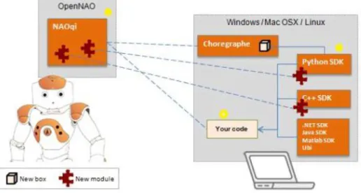
This section describes the software architecture and tools available for programing the robot. Aldebaran robotics provides a comprehensive software development kit that enables the development of applications for the robot by experts and novices. Nao SDK packages provide a means for professionals to develop applications for the Nao robot using supported programming languages. For the ease of programming, Aldebaran robotics provides a visual programming interface named Choregraphe. This GUI application includes the libraries of predefined blocks for simple robot tasks. It also enables users to control the robot by combining a set predefined and easily customizable blocks to form compound blocks that make up a complete and functional program sequence.

The software for Nao robot can be classified into two types: embedded software and desktop software. The embedded software runs on the motherboard located in the head of the robot and it is responsible for Nao’s autonomous behavior. The operating system

(26)

of the robot is referred to as OpenNao. It is a Gentoo Linux distribution specifically developed for the Nao robot’s needs. It provides all the libraries and modules required by Naoqi, another software that governs the behavior of the robot.

The desktop software runs on the user’s computer. This software enables the programmer to create new behaviors and to control the robot remotely. It provides a link between the user’s developed application and the Naoqi software running on the robot.

Fig 3.5. Nao Software Interaction

3.3.1 Naoqi framework

Naoqi is a distributed software framework that governs the behavior of the robot. It runs on the OpenNao operating system and it can also be run on the computer in a virtual simulator of the Nao robot, called webots. Robot functionality is encapsulated in software modules, so users can communicate to specific modules in order to access sensors and actuators. Communication between user defined modules and inbuilt modules are provided by the framework.

Naoqi framework currently supports five programming languages: C++, Python, URBI, Java and Matlab. It has also been tested in the Microsoft .Net framework for C#, F# and Visual Basic programming language. Amongst the specified programming languages, Python and C++ are the most developed for Nao. Programs written in C++ or Python

(27)

can be installed and run directly on the robot and remotely, whereas all other supported languages are supported only on the desktop computer.

This framework comprises a set of modules, e.g. memory, motion, vision, sonar and device communication manager (DCM). It functions as a broker by allowing homogenous communication between modules and sharing of information on resource availability. Thus the modules can access methods from other modules across the network. This communication enables capability for parallelism and synchronization. Naoqi also provides capability for monitoring the state of memory values. When the value at a memory location is changed, an event is raised and the appropriate action specified in the case of this specific event is carried out.

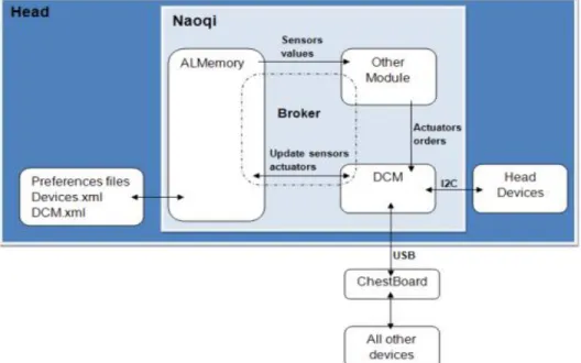
Figure 3.6. Naoqi Framework

Although Naoqi is a very useful framework, the software is still under development and several of the provided modules lack adequate documentation on programming.

In the implementations carried out in this thesis, an attempt was made to use a third party integrated development environment (IDE) for programming. The result was disappointing because some predefined methods within Naoqi modules were unresponsive. The support provided by the Aldebaran robotics community online was insufficient for resolving all the problems.

(28)

3.3.2 Device communication manager (DCM)

The device communication manager is a software module that manages communication with all electronic devices in the robot. It controls the robot directly by sending command calls to the robot’s ARM controller, a type of processor based on a reduced instruction set computing architecture. The DCM is a link between the higher level architecture Naoqi and low level devices such as actuators and sensors. This includes electronic boards, joint position sensors and actuators. Devices such as the microphone, speakers, and camera are excluded from the DCM tasks. These devices are connected directly to head’s on-board system. The DCM is essential for real-time processes such as access to image data, when a new image is captured by robot’s camera, or for generating walk sequences. Modules for motion are designed to interact directly with actuators using the DCM while the extractor modules retrieve values from memory through the DCM. One pitfall in using the DCM is that robot stability is disabled when interacting directly and as such stability has to be ensured by the programmer.

3.3.3 Nao Simulation Environment

The GUI programming environment Choregraphe is also useful when a real robot is not available. It comes with a simulated Nao having features of the real robot, excluding functions that require the exteroceptive sensors are not available on the simulated robot. Programming is done through drag-and-drop, and by connecting graphically the function blocks.

An alternative robot simulation environment is webots, a third party application developed specifically for Nao robot. This offers simulation in a customizable virtual world, where all sensor, also the ones excluded in Choregraphe, are available to the user.

(29)

Figure 3.7. Screenshot of the Choregraphe software.

3.4 Motion

The motion module provides methods that enable the robot to move. It creates a “motion task” anytime a call to produce a movement is made through the API. The motion task computes the elementary commands to change motor angles and stiffness. The commands are scheduled such that they are performed only when the requested resources are available. The methods are categorized into four major groups: joint stiffness control, joint position control, locomotion control and Cartesian control methods. Within the motion module, safety measures such as self-collision avoidance, fall manager and smart stiffness are implemented.

In order to apply the motion module, the user is required to create a proxy for the module using Naoqi brokers. This proxy makes all methods within the module available to the user.

The joint stiffness control determines the torque to be generated when the robot is initialized for a motion task. The value of stiffness ranges between 0 and 1. A joint is compliant when the stiffness is set to 0 and it rigid when the stiffness value is 1. One important aspect of the motion module is that without setting stiffness “ON” any motion command specified to the module will remain unresponsive.

(30)

The joint position control comprises dedicated methods for controlling the position of Nao’s joint. Each joint can be controlled individually by specifying the joint name or in parallel with other joints by specifying a chain name, where a chain would represent a group of joints such as “Body”.

The Cartesian control is dedicated to controlling the effectors of the robot in Cartesian space using an inverse kinematics solver.

The Locomotion control comprises methods which make the robot move to places. Some of the methods for locomotion control are listed below.

· ALMotionProxy::moveTo (x, y, Ө), to set a target pose relative to the present pose, that Nao will walk to. The robot computes the required sequence of actions to reach the target.

· ALMotionProxy::move (direction, intensity) is used to set Nao’s instantaneous velocity in SI units. This is usually used to control the walk from a loop with an external input such as visual tracker.

· ALMotionProxy::moveToward (direction, intensity) is used to set Nao’s instantaneous normalized velocity. It is typically used to control the robot from a joystick.

· ALMotionProxy::setWalkTargetVelocity (direction, intensity) is used to set Nao’s instantaneous normalized step length and frequency, and thus control its velocity indirectly.

3.5 Vision

NAO’s vision system has modules for face detection, movement detection, landmark detection, visual compass, photo capture and red ball detection. The landmark detection module is utilized for this thesis. This module enables the robot to recognize special landmarks referred to as Naomarks.

Naomark consists of black circles with white triangle fans centered within the circle. The size, orientation and location of each fan on the triangle are used as a distinguishing feature for each Naomark. The range of detection for Naomark is accurate to about 2 meters and when the angle of view is less than 60 degrees.

(31)

Once the landmark detection module is subscribed to, the robot camera is activated. The detection of Naomark by the robot camera produces the landmark information that is stored in the robot memory. Each detection provides the following information; Marker ID, angle alpha and beta in radians representing the location of the center of the detected marker in terms of camera angles measured from the center of the field of view, and size - x and size - y i.e. the marker size in camera angles.

The landmark detection module is useful for distance measurements. Since the other available sensors are not suited for distance measurements, landmark detection provides an alternative approach for measuring the distance to a reference point relative to the robot. This capability makes it vital for localization.

(32)

4 METHODOLOGY AND

IMPLEMENTATION

This chapter describes the methods for data acquisition, interpretation and transformation into useful information for robot localization. It also covers the algorithms and techniques used for determining the path which the robot uses in reaching its set objective.

4.1 Motion tests

A set of tests was carried out to ascertain the behavior of the Nao robot given a walk or turn command. The Nao robot was commanded to turn an angle ( ) and move a specific distance (r). The start pose of the robot ( , , ) and the end pose after each action were measured. The data from the experiment provides a means to determine the walk length of Nao within which odometer measurements can be relied on and the nature of the uncertainty in walk. These measurements provide data about the behavior of the robot when commanded to walk or turn a certain value. From the measurements, the process/motion noise values were determined.

4.1.1 Distance Measurements

Measurements were carried out for walks of distances 50 cm, 100 cm and 200 cm respectively, starting from a point (x, y) chosen as the origin (0, 0). The robot was commanded to the specified distances in the robot’s x-direction after which the covered distance and displacement from the walk path was measured. The outcome of these measurements showed that the lateral displacement mostly tends to the positive y-direction and the distance covered in the x-y-direction is lower when the lateral displacement is high. The x-coordinate and y-coordinate of the robot and finally the heading of the robot phi (ф) was recorded. Table 4.1 shows some of the recorded values.

(33)

Table 4.1. Walk measurements Distance along x . ± . cm . ± . cm . ± . cm 1 50.0 99.2 188.5 2 50.5 100.8 185.5 3 50.4 99.2 205.2 4 50.5 100.4 200.0 5 50.5 102.7 203.7 6 51.0 100.8 201.4 7 50.5 99.6 201.8 8 50.3 99.2 201.8 9 51.4 99.6 194.9 10 50.8 101.3 201.3

4.1.2 Turn Measurements

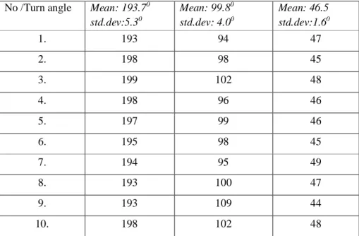
Turn measurements were carried out by making the robot turn an angles pi/4, pi/2 and pi at a point and the value of the output was recorded for twenty trials. The amount of overturn or under turn, and the robots displacement from the center point were recorded. It was observed during measurements that the robot mostly overturns for each of the specified turn angles. Furthermore, the turn increases in proportion to the specified turn angle. This provides some idea for determining a suitable value for bias and uncertainty in turn. Even so, the uncertainty in turn was determined to be a Gaussian distributed random value within means specified as the commanded turn angle and a variance given by the range of the error in turn. Table 4.2 shows the some of the values for turn measurements in each case.

(34)

Table 4.2: Robot turn measurements for angles 180, 90 and 45 degrees

No /Turn angle Mean: 193.70

std.dev:5.30 Mean: 99.80 std.dev: 4.00 Mean: 46.5 std.dev:1.60 1. 193 94 47 2. 198 98 45 3. 199 102 48 4. 198 96 46 5. 197 99 46 6. 195 98 45 7. 194 95 49 8. 193 100 47 9. 193 109 44 10. 198 102 48

4.1.3 Straightness measurements

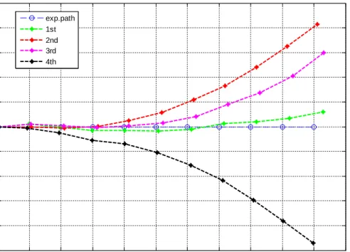
Further test was carried out to determine the walk path for a 200 cm straight walk command. The (x, y) positions of the robot on a plane were recorded for every 20cm walk sequence for a total distance of 200 cm. The straightness measurements were repeated four times to illustrate how much the robot deviates from specified walk path at each walk. The result of the above measurements is vital for determining the optimal walk distance that limits the accumulated error in walk.

Figure 4.1 below shows a plot of the straightness measurement for four walks. The requested path is shown with the blue markings dotted line while actual paths are shown as 1st, 2nd, 3rd and 4th.

(35)

Figure 4.1. Walk path of Nao robot for 200cm command along x-axis.

4.2 Visual markers

The vision aspect of this work utilizes naomarks. The vision module of the robot already provides ability to recognize naomarks, red balls and faces. For localization, the landmark detection module is applied for determining the location of the naomark relative to the robot. The following sections describe the approach.

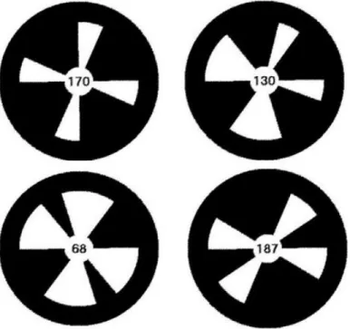
4.2.1 Naomarks

Aldebaran robotics provides a total of 29 markers. Each of these markers has a unique shape that distinguishes it. A marker is a black circle with a white pattern it. Encoded in the shape of the white pattern is the unique identity of the marker. The landmark detection module provides a means to acquire information from these markers when detected by nao camera. Practically, the robot can detect shape of the markers, the distance of the marker from the robot camera, and the unique ID of the marker. Using

0 20 40 60 80 100 120 140 160 180 200 220 -50 -40 -30 -20 -10 0 10 20 30 40 50

Nao's 200 cm Straight Walk Along X

Y -d e v ia ti o n c m X cm exp.path 1st 2nd 3rd 4th

(36)

the associated desktop monitor software, users can see the marker and the ID as detected by the robot.

Figure 4.2. Naomarks samples

4.2.2 Limitations of the landmark module

Although the landmark detection module offers a simple approach to visual localization, there exist several limitations to its application. This module is plagued by the quality of the images acquired by the camera. As stated in the documentation, the first key requirement is sufficient illumination. The detection relies on contrast differences in the image. The proper illumination must be between 100 Lux and 500 Lux. Lighting conditions below this range often results in misidentification of markers or no detection in the worst case.

Secondly the tilt of the marker’s plane relative to the camera must be between +/- 60 degrees for detectability. For optimal performance, the naomark must be in the direct line of sight of the robot. Experiment performed on the robot using both cameras showed no detection for landmark placed on the floor plane, while the landmark placed on the walls were detected albeit some misclassifications.

(37)

The third limitation is the size of the marker within the image and the range of detection by the camera. The minimum size is approximate 0.035 rad which corresponds to 14 Pixels in a QVGA image, while the maximum size is approximately 0.40 rad or 160 pixels within the QVGA image. At this marker image size ranges and marker real size being 108.54 mm, the distance range for detection is from 30 cm to about 200cm.

4.2.3 Landmark

detection info

The data for detected landmark is obtained directly from the robot’s memory using the memory proxy’s getData ( ) method. The data for any observation is structured as follows.

ALLandMarkDetectionInfo {

TimeStamp, MarkInfo [N], CameraPoseInNaoSpace, CameraPoseInWorldSpace, CurrentCameraName }

The Timestamp field contains the time at which a landmark was detected in the image from the robot camera. The MarkInfo [N] is the list of N landmarks detected and it contains detailed information such as shape information and Marker Id. The MarkerInfo field is structured as follows:

MarkInfo {

ShapeInfo, MarkerId }

The MarkerId is the number written on naomark which corresponds to its pattern.

ShapeInfo {

heading, alpha, beta, sizeX, sizeY }

The shape info field contains the heading angle this describes the orientation of the naomark about the vertical axis. The field alpha and beta represents the naomark’s center in terms of camera angles in radian while sizeX and sizeY are the camera angles.

(38)

The CameraPoseInNaoSpace and CameraPoseInWorldSpace expresses the 3d vector and pose angles of the camera with respect to the robot and to the world when the image was captured. Finally the CurrentCameraName can be either the “CameraTop” or “CameraBottom” indicating which camera was used for image acquisition.

4.2.4 Marker coordinates

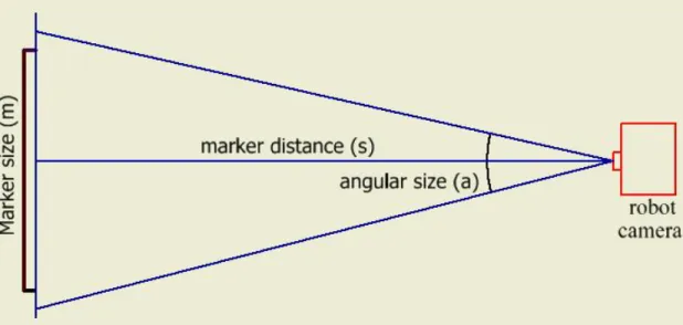
The coordinates of the marker acquired by the robot camera are computed using the shape info. First we need to know the physical dimension of the naomark detected. With this we can calculate the distance of the marker from the robot using the following steps.

Figure 4.3. Naomark dimension

The variable (S) is the distance of the marker from the camera can be calculated using the angular size (a) and the marker size (m) as show in the following equation. The marker size is the size of the printed marker. For this experiment, the size is 108mm. The parameters sizeX and sizeY, for which identical values are given in the image of detected markers, are the dimension from center-most to the edge on the horizontal and vertical image axis respectively.

(39)

Figure 4.4. Nao Camera angles

= 2

atan ₂ (1)

The angles alpha and beta are used to obtain the transformation from the robot frame to the landmark. To obtain the coordinate of the marker in the robot frame, a transformation from camera frame to the robot frame is required. This transformation is performed using methods defined in the transform class of the implementation.

The computation for this transformation is presented in equation (2)

= ∗

∗ (2)

The result is a transformation matrix which includes the (x, y, z) coordinates of the landmark in the robot frame. Since we are concerned only with the position horizontal distance of the landmark from the robot, the z-coordinate is ignored in future applications.

(40)

4.3 Environment map

The environment map was built using a set of 13 known markers. The environment is designed as a 2 m x 2 m area. Each marker was located in the map at specific coordinates, as shown in the table below.

Table 4.3. Global coordinate of markers on map

Marker ID x-position (cm) y-position (cm)

170 200 55 141 125 0 112 0 50 117 0 100 131 200 118 130 70 0 138 0 150 108 0 180 175 200 40 125 200 90 127 145 200 109 200 166 146 26 200 80 60 200 143 102 200 124 180 200 119 175 0 171 25 0

4.4. Visual localization

The location and orientation of the robot in the global frame are determined based on the 2D relative coordinates of markers detected by robot in robot frame and the coordinates of same markers in global frame. Earlier experiments carried out by [12] provide a proof of the approach. This section describes the approach developed by [12] and how the pose of the robot is determined.

First the transformation between the global and local frame of the robot is outlined. The robot has its X axis from the robot pointing forwards and Y axis direction pointing to the left of the robot. Figure 4.5 shows NAO’s frame and the global frame together.

(41)

Figure 4.5. Nao Frame and global frame

The 2D transformation between the robot frame of marker and the global frame is a combination of rotation and translation. This is shown in equation (3).

X

_global

Y

_global

=

cos

φ

sin

φ

−

sin

φ

cos

φ

X

_robot

Y

_robot

+

X

₀

Y

₀

(3)

The subscripts “global” indicates coordinates of the marker in the global frame, “robot” indicates coordinate of the marker in the robot frame while X0 and Y0 are the robot

location in the global frame. The angle denotes the orientation of the robot in the global frame. The equation can be rewritten in a more compact form as:

⎝ ⎜ ⎛

X

_global

Y

_global 1 ⎠ ⎟ ⎞ = ⎝ ⎜ ⎜ ⎛

cos

φ

- sin

φ

X

₀

sin

φ

0

cos

φ

0

Y

₀ 1 ⎠ ⎟ ⎟ ⎞ ⎝ ⎜ ⎛

X

_robot

Y

_robot 1 ⎠ ⎟ ⎞ (4)

(42)

Since equation (3) has three unknowns the knowledge of relative coordinates and global coordinates of one marker alone is not sufficient to determine the location and orientation of the robot in the global map. If the coordinates of at least two markers are known and assuming that the position of the robot remains unchanged during detection of the markers, two sets of equations for the two detected marker coordinates would provide four equations with three unknowns, the robot’s coordinates and orientation. An illustration of is shown in figure 4.6. The equations for two marker case read as:

Figure 4.6. Representation of marker locations in global and robot frame

⎝ ⎜ ⎛

X1

_global

Y1

global 1 ⎠ ⎟ ⎞ = ⎝ ⎜ ⎜ ⎛

cos

φ

- sin

φ

X

₀

sin

φ

0

cos

φ

0

Y

₀ 1⎠ ⎟ ⎟ ⎞ ⎝ ⎜ ⎛

X1

_robot

Y1

robot 1 ⎠ ⎟ ⎞

(5)

⎝ ⎜ ⎛

X2

global

Y2

_global 1 ⎠ ⎟ ⎞ = ⎝ ⎜ ⎜ ⎛

cos

φ

- sin

φ

X

₀

sin

φ

0

cos

φ

0

Y

₀ 1⎠ ⎟ ⎟ ⎞ ⎝ ⎜ ⎛

X2

_robot

Y2

_robot 1 ⎠ ⎟ ⎞ (6)

These four equations have three unknowns and thus the system is overdetermined. One simple way to deal with this is consider andsin as independent variables, and the check their constraint after solution. The two landmarks for localization should be at

(43)

a considerable distance from each other, and the markers must not be coplanar otherwise the errors in pose estimation would be significant. These conditions present a challenge to the localization, since the landmark detection range is limited by the camera field of view and the marker tilt range. A solution to these is to rotate the head of the robot by a specific angle (0 ± ) during marker detection and then carry out a transformation of the relative marker coordinates by angle (0∓ ) during localization. The localization scheme is presented in Pseudo code 4.1

1 Begin

2 Obtain a list of marker coordinate in robot frame. 3 For any pair of markers:

4 If they have different X and Y with each other (non-coplanar)

5 Solve coupled equations and get the pose of robot for the two markers. 6 If pose is within limits of map

7 Update pose list

8 End if

9 else if they have the same X and Y (coplanar) 10 Transform coordinates of marker, go to line 5 11 End if

11 End

12 determine average over robot pose list 13 End

Pseudo code 4.1. Determining robot pose

The implementation in line (4 – 6) deals with non-coplanar marker conditions required for accurate pose estimation and the solution the set of equations for the selected markers. Lines (7 - 9) checks that the computed pose is within specified limits in terms of map area and for the orientation between –pi < value < pi. If the condition is met, the pose is update to a list of poses from which an average pose is determined in line (11).

The parametersX0, Y0and from equations 5 and 6 can be solved either by using C++

library for symbolic named “symbolic C++” or analytically. For this work, the analytic approach was chosen due to missing dependencies in Linux GCC library required by Symbolic C++. The expression for X0, Y0and and is shown in equations

(44)

of the landmarks while , , the represents coordinates of landmarks in robot frame. = −( − − + − + + + − − + + ) (( − )( − ) + ( − )( − )) (7) = −(− + + − + − + − − + + + ) (( − )( − ) + ( − )( − )) (8) =−( ( ₍₍− ₋) + ₎₍( ₋− ₎) +₊ ₍ (₋ −₎₍ ) +₋ ₎₎( − )) (9a) = −( ( ₍₍− ₋) + ₎₍( ₋− ₎) + (₊ ₍ ₋ −₎₍ ) +₋ (₎₎ − )) (9b)

For a planar robot the orientation in world frame can be described as 0 ≤ ≤ or − ≤ ≤0 Since arc-cosine provides results in this range, the cosine results from equation (9a) is relied upon for orientation values.

An important observation made in the course of experiments was that, when the robot is at very close proximity (< 30 cm) to landmarks the visual localization the estimates of robots position and orientation are largely inconsistent.

(45)

4.5. Implementation of Particle filter based localization

This section describes application of the particle filter for localization on the Nao robot. The basic particle filter has four steps.

· Initialization · Prediction

· Measurement update · Resampling

First a set of samples or random particles representing the beliefs of the robot state is created within the confines of the map. For the prediction step, a motion model that simulates the movement of the robot on each particle is determined. The particles in this step are evolved based on the robots motion model. The next step is the measurement update. Here weights are assigned to each particle based on information from sensors. The weights are normalized such that particles well-compatible with the sensor data – in this case marker-based localization – are highly weighted, while particles less compatible with data are assigned low weights. The last step is the resampling. The idea of the resampling step is simply that particles with very low weights are abandoned, while particles with high weights are retained and replicated. In order that the total number of particles is maintained, identical copies of high-weighted particles are formed. This is referred to as sampling with replacement.

4.5.1. Motion Model

At the prediction stage, the effect of control or command on the pose of the robot is modelled by applying the control action on Nao’s motion model. First, consider the control or action required to produce a motion on the robot. Given Nao’s pose on the plane as [ , , ] where( , )is the position of Nao in world coordinates and is the orientation of the robot coordinate system. The effect of changes [∆ ∆ ] in the robots position on the plane can be described by a rotation followed by a translation.

The robot rotates ∆ = ( )− ( −1). Where ( ) = arctan(∆ _∆ ) and then translates the distance = ∆ + ∆ to its destination. The location and orientation of the robot after every control inputk is given by:

(46)

( ) = ( −1) + ( )cos ∆ ( ) ( ) = ( −1) + ( )sin ∆ ( ) ( ) = ( −1) + ∆ ( )

(11)

In order to predict the probability distribution of the pose of the robot after each motion, the effect of noise on the process must be modelled. For both the translational and rotational motion robot the noise are modelled as an additive Gaussian noise.

The turn noise is modelled as a Gaussian ( , ) with mean with the men rotational error and variance determined through the experiments in section 4.1.2

The translational noise arises from two sources. The first is the error in distance travelled and the second is the changes in orientation during translational motion. The changes in orientation during translation are responsible for robot’s deviation from the desired direction of translation (lateral translation). The error due to distance is travelled was determined through experiments in section 4.1.1. Analytical modelling of the deviation of the second noise parameter is difficult, so the approach chosen was to limit the distance moved at each step to 50cm and then model the noise as a Gaussian with ( , ). So at each walk of 50cm the robot is assumed to have deviated with a mean value of , and a variance .

Thus the motion model including the noise is given by:

( ) = ( −1) + [ + ( , )]( )cos( + ( , )))( ) ( ) = ( −1) + [ + ( , )]( )sin( + ( , ))( ) ( ) = ( −1) + [ + ( , )+]( )

(47)

4.5.2. Measurement and updates

To determine the weight of each sample in the particle filter, a measurement of the robot’s location and orientation is obtained from observation of landmarks. The observations are coordinates of landmarks in robot frame. The visual localization process described in Section 4.4 provides the measured location of the robot in the global map. The measurement from the sensor is assumed to be noisy and thus the measured location and orientation of the robot is subject to measurement noise.

The probability of each sample particle is computed using the difference in Cartesian coordinates and orientation of the particles and the measured location.

The probability is computed as shown:

) = 1 2 −(∆ ) 2 1 2 −(∆ ) 2 1 2 ∅ −(∆ ) 2 _∅ (13)

Where represent the probability ofi-th particle given the measurement . ∆ = − , ∆ = − , and ∆ = −

The constants and _∅ are the measurement noise and they indicate the confidence with which we weight each measurement in terms of the terms of position and orientation.

4.5.3. Resampling

The resampling step adopts sampling with replacement. The process of resampling is described in the Algorithm 1. First the cumulative sum of particle weights is computed, then a random numbers selected from a uniformly distributed set in the range [0, 1]. The next step applies the resampling algorithm described in [13].

Algorithm 1 below presents a formal description of the “select with replacement” algorithm. The resampling produces a new set of particles that describes the next state of the robot.

(48)

Algorithm 1: Select with replacement sampling algorithm 1: Input: floats [ ], [ ]

2: = ( ) {Cumulative sum of weights =∑ }

3: = ([0,1])∗ {Select a random index from the set of particles}

4: = 0.0 5: = ( ) {Maximum weight} 6: 7: = + ([0,1])∗ 2 ∗ 8: ℎ ( > ( )) 9: = − [ ] 10: = ( + 1)% 11: Output: [ ]

4.6. Motion planning

This section deals with robots movement from its initial position to a specified target position with obstacle present in unknown locations. Motion planning utilizes Nao sensors to determine how the Nao would reach its target. The bumper sensors on the Nao’s feet are used to detect obstacles at collision. Initially the path is assumed to be free from obstacles and so the initial plan of the robot is a straight walk to the target. Figure 4.7 shows the robot and the target in 2D plane.

First, the direction of the target is determined based on the robot orientation and the target coordinates on the map. The turn angle required to align the robots heading to target direction is determined. Next the shortest angle to achieve the alignment is computed. The difference in heading between the target and the robot is specified as the turn angle of the robot.

(49)

Figure 4.7. Illustration of robot and with a specified target coordinate.

= arctan (15)

The Euclidean distance between the robot and the target is computed using equation 16.

= − + ( − ) (16)

The robot moves in the set direction until it collides with an obstacle. On collision, the robot stops and computes the distance covered prior to collision. The location of the obstacle is determined using odometry readings. Then the robot evades the obstacle by taking the following actions. First the robot steps back a few steps, randomly turns an angle pi/6 either to the left or right direction, then moves forwards a distance equivalent to twice the backward steps. Next the robot re-localizes and computes new turn angle and distance to target. If the robot is at target it stops; if the robot is still away from the target, then a turn and move action is perfumed to guide robot from present state to target. The program flow is described by the flow chart in Figure 4.8.

(50)

Figure 4.8. Flow-chart of the navigation and localization program

At initialization, Nao is set to a stand posture then particles are created and the target point is specified. Next the robot localizes by calling the landmark detection module and using equations (15) and (16). Then the robot calculates the difference between its pose and the target specified. If the difference greater than a specified tolerance, the

On particle filter localization and mapping for Nao robot