Local features for visual object matching and video scene detection

(1)

LOCAL FEATURES FOR VISUAL OBJECT MATCHING AND

VIDEO SCENE DETECTION

Master’s Thesis

Examiners: Professor Joni-Kristian Kämäräinen

Examiners and topic approved in the Computing and Elec-trical Engineering Faculty Council meeting on 4th Novem-ber 2015

(2)

TAMPERE UNIVERSITY OF TECHNOLOGY

Master’s Degree Programme in Information Technology

ANTTI HIETANEN: Local features for visual object matching and video scene de-tection

Master of Science Thesis, 63 pages September 2015

Major: Signal Processing

Examiner: Prof. Joni-Kristian Kämäräinen

Keywords: Local features, Feature detector, Feature descriptor, Object class matching, Scene boundary detection

Local features are important building blocks for many computer vision algorithms such as visual object alignment, object recognition, and content-based image retrieval. Local features are extracted from an image by a local feature detector and then the detected features are encoded using a local feature descriptor. The resulting features based on the descriptors, such as histograms or binary strings, are used in matching to find similar features between objects in images.

In this thesis, we deal with two research problem in the context of local features for object detection: we extend the original local feature detector and descriptor performance benchmarks from the wide baseline setting to the intra-class matching; and propose local features for consumer video scene boundary detection.

In the intra-class matching, the visual appearance of objects semantic class can be very different (e.g., Harley Davidson and Scooter in the same motorbike class) and making the task more difficult than wide baseline matching. The performance of different local feature detectors and descriptors are evaluated over three different image databases and results for more advance analysis are reported.

In the second part of the thesis, we study the use of Bag-of-Words (BoW) in the video scene boundary detection. In literature there have been several approaches to the task exploiting the local features, but based on the author’s knowledge, none of them are prac-tical in an online processing of user videos. We introduce an online BoW based scene boundary detector using a dynamic codebook, study the optimal parameters for the detec-tor and compare our method to the existing methods. Precision and recall curves are used as a performance metric.

The goal of this thesis is to find the best local feature detector and descriptor for intra-class matching and develop a novel scene boundary detection method for online applications.

(3)

TIIVISTELMÄ

TAMPEREEN TEKNILLINEN YLIOPISTO Tietotekniikan koulutusohjelma

ANTTI HIETANEN:Paikalliset piirteet visuaalisten objektien luokittelussa ja vide-on otosten leikkauskohtien tunnistamisessa

Diplomityö, 63 sivua Syyskuu 2015

Pääaine: Signaalinkäsittely

Tarkastaja: Prof. Joni-Kristian Kämäräinen

Avainsanat: Paikallinen piirre, Piirrehavaitsin, Piirrekuvaaja, Objektiluokkien sa-mankaltaisuuden tunnistaminen, Otosten leikkauskohtien tunnistus

Paikalliset piirteet ja niiden kuvaajat ovat tärkeitä komponentteja monessa tietokonenä-köön liittyvissä algoritmeissa kuten visuaalisten objektien kohdistamisessa, visuaalisten piirteiden tunnistamisessa ja sisältöpohjaisen informaation haussa. Paikalliset piirteet ir-roitetaan kuvasta piirreirroittimen avulla ja tämän jälkeen nämä piirteet koodataan piir-rekuvaajan avulla. Piirrekuvaukset voivat olla esimerkiksi histogrammeja tai binäärisiä merkkijonoja, joita käytetään samankaltaisten piirteiden tunnistamisessa objekteista kah-den eri kuvan välillä.

Tässä opinnäytetyössä tutkimme kahta eri ongelmaa liittyen paikallisten piirteiden käyt-tämiseen objektien tunnistamisessa: laajennamme alkuperäistä paikallisten piirteiden ha-vaitsijoiden ja kuvaajien suorituskyvyn testausmenetelmää samasta objektista samaan luokkaan kuuluvien objektien tunnistamiseen ja hyödynnämme paikallisia piirteitä leik-kauskohtien tunnistamiseen videosta.

Saman luokan sisäisten objektien ulkomuoto voi olla hyvinkin eri näköinen (esimerkik-si moottoripyöräluokan aliluokat Harley Davidson ja skootteri) ja täten tekee objektien tunnistamisesta hankalempaa kuin saman objektin tunnistamisesta eri ympäristössä. Eri piirteen havaitsijoiden ja kuvaajien suorituskyky arvioidaan työssä kolmen eri tietokannan avulla ja tuloksia analysoidaan yksityiskohtaisesti.

Opinnäytetyön toinen osa koostuu "piirrelaukku-menetelmän tutkimisesta ja sen hyödyn-tämisestä videon eri leikkauskohtien tunnistamisessa. Kirjallisuudessa on esiintynyt muu-tamia menetelmiä tehtävän ratkaisemiseksi hyödyntäen paikallisia piirteitä, mutta mikään niistä ei ole käytännöllinen online-järjestelmän kannalta. Seuraavien kappaleiden aikana esittelemme uuden piirrelaukku-menetelmän videoleikkausten tunnistamiseen hyödyn-täen muuttuvaa koodikirjastoa, etsimme optimaaliset parametrit menetelmälle ja vertaam-me sitä jo olemassa oleviin vertaam-menetelmiin. Suorituskyvyn mittaamiseen käytämvertaam-me "preci-sion and recall"käyrää.

Tämän opinnäytetyön tavoite on löytää paras piirrehavaitsin ja -kuvaaja tunnistamaan eri objektit samasta luokasta ja kehittää uudenlainen leikkauskohtien tunnistusmenetelmä re-aaliaikaisia järjestelmiä varten.

(4)

First of all, I wish to thank my supervisor Professor Joni-Kristian Kämäräinen for giving me an opportunity to work in his research group and for his guidance and patience during the work. I wish to also thank Jukka Lankinen D.Sc. (Tech) for his help and support. I want to thank the whole computer vision group at Tampere University of Technology providing an enjoyable work environment.

Finally, I want to thank my family and especially my love, Pinja.

Tampere, September 21th, 2015

(5)

ABBREVIATIONS AND SYMBOLS

σ Gaussian kernel size

σn Number of edge pixels in framen

λ1 Eigenvalue calculated formM

λ2 Eigenvalue calculated formM

τ Threshold value

τ(P;x,y) Binary test in BRIEF

0 Overlap error

θ Orientation

b Color component

ci Correspondence score

ECRn Edge change ration in framen

F F-measure D(x, σ) Difference-of-Gaussian G(x, kσ) Gaussian kernel g Color component Det Determinant H Hessian matrix

H Tomography of two images

L(x) Intensity function of Gaussian smoothed image Lx(x) Partial derivative in x direction ofI(x)

Ly(y) Partial derivative in y direction ofI(x)

Lxx(x) Second-order partial derivative in x direction ofIx(x) Lxy(x) Second-order partial derivative in y direction ofIx(x) Lyy(x) Second-order partial derivative in y direction ofIy(x)

C Centroid of a patch

K Number of best matches

M Second moment matrix

mi Number of matches

mpq Moment of a patch in ORB detector

N Number of correct matches in Coverage-N measurement

P Patch in BRIEF

P Precision

Rµ Detected elliptic region

R Recall

r Color component

(8)

x Coordinate point

T Threshold value

T r Trace

Xin

n Number of entering edge pixels in framen X_nout₋₁ Number of exiting edge pixels in framen−1

2D Two dimensional

3D Three dimensional

BoW Bag-of-Words

BoF Bag-of-Features

BRIEF Binary Robust Independent Elementary Features

DoG Difference-of-Gaussian

HoG Histogram of Oriented Gradients

LoG Laplacian-of-Gaussian

NIST National Institute of Standards and Technology

ORB Oriented BRIEF

PCA Principal Component Analysis

RGB Red-Green-Blue Color Space

SIFT Scale-Invariant Feature Transform

SVM Support Vector Machine

(9)

1 INTRODUCTION

As humans, we have powerful ability to perceive the three-dimensional world around us. You can immediately recognise different flowers from the vase and maybe even name their sort. Looking at unfamiliar object, for instance an animal or food, you can draw a conclusion of the target by comparing it to your earlier experiences with objects having similar colour, texture or shape appearance. There have been a great deal of work trying to understand how the human visual system works but the solution remain still unaccom-plished [1].

Despite the difficulties in modelling human visual system, over the years there have been significant progress in the field of computer vision [2, 3]. Development of computer vision have given us great potential to change the way we interact with computers and help us to augment the physical real-world. Researchers have developed mathematical techniques which computers utilize for recovering the three-dimensional shape and appearance of objects in images. We have already made reliable techniques to make panoramic view of an environment from thousands of partially overlapping photographs. Another pop-ular application is for instance face recognition which can be found from social media applications and surveillance systems.

In Figure 1 is shown some active topics of the field of computer vision during different decades. In the 1970s the computer vision was distinguished from the common image

(10)

processing by the desire of recovering the three-dimensional structure of the world from images and use this information to full scene understanding. The earliest attempts to ex-tract information from the scene was exex-tracting edges and then inferring the 3D structure of an object or a "block world" from the topological structure of the 2D lines [4].

In the 1980s lot of efforts was putted to improve existing algorithms and mathematical techniques. Moravec [5] introducedinterest operator based on the intensity variation in the local neighbourhood of a pixel. Harris and Stephen improved this method in 1988 by presenting theHarrisdetector [6].

One of the most noteworthy result achieved in the 1990s was development in the area of image-based modelling and rendering due to progress on computer graphics [7] which lead to numerous image manipulation techniques such as image morphing and view in-terpolation.

Interest points and other feature-based techniques have been the trend for object recogni-tion during the 1900s and the 2000s. Many successful approaches have been presented, such as SIFT [8], which was well accepted and is still used in many works as a baseline for new approaches. One of the active topics of 2000s werecategory-levelorintra-class object recognition [9, 10, 11], where the problem is to classify an object to a particular general class such as "dog", "car" or "bicycle". A popular algorithm for category recog-nition is the Bag-of-Words (also noted as Bag-of-Features, Bag-of-Keypoints, and BoW) approach, where the term bag of keypoints was first used in 2004 by Csurka et al. [9]. During this decade more and more interest have gained the deep neural architectures [12].

1.1 Object recognition using local features

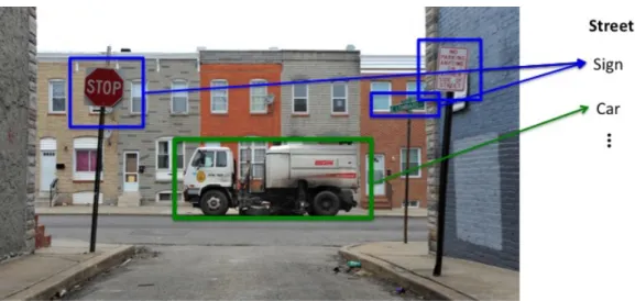
In literature, the termrecognitionor generallydetectionrefers to detecting an instance of a particular object class under many viewing conditions in unconstrained settings (Figure 2). A common way is to extract local features by a feature detector, encode them into descriptions by a feature descriptor, and use the descriptions as an input data for certain task such as object categorization or image stitching.

(11)

Figure 2. An example of object recognition.

1.1.1 Local features

A local feature is an image pattern which differs from its immediate neighbourhood [13], for instance a point on an image where a small shift in multiple directions result large intensity changes in the texture. In addition to texture, changes in other image properties, such as colour, can result an interest point depending on an algorithm. These detected interest points are then encoded by a feature descriptor todescriptions, which are ultimate feature of an application.

Why someone should use local features? One could be interested in specific type of features: in the earlier development of local features, they were used to detect corners and edges, such as the Harris detector [6]. A typical application could be a detection of road edges from an aerial image. Secondly, one might not be interested in the actual representation of an interest point itself, more like the accurate location of it and that it can be found under various transformations. Depending on a algorithm, local features can provide different type of features and be robust to various image transformations and hence local features are used as anchor points needed in many matching tasks, for example, in object retrieval [10, 14, 15] and mosaicing [16]. Thirdly, slightly related to the second point, using local features allows us to detect objects without segmentation because local features are highly tolerant to occlusion and clutter which are the main reason for segmentation.

(12)

1.1.2 Local features in visual object categorization

In visual object categorization (VOC), the task is to find category for an object in a given image. The task can be hard due to numerous transformations in the image (described in Section 1.1.3) and presence of multiple instances of the same and different category objects in the image. VOC methods can be divided into two different learning approaches: unsupervisedandsupervised.

• Supervised: Before the actual detecting process, a subset of local features from object category are used to train a model which represent instances of this object category. The model should be as discriminative as possible in order to distinguish two or more different categories.

• Unsupervised: In a unsupervised approach, we are not provided local features with correct category labels to train the model. The task is to find the hidden characteris-tics of the object category, which makes the unsupervised learning more challenging task than supervised.

Why then to choose unsupervised learning? In real life tasks the common unambiguous characters of some object category are not know or they are impossible or impractical to attain. Also by unsupervised learning one can explore data that is considered to be purely unstructured and find hidden patterns from there.

A typical unsupervised approach is to cluster unseen data to different clusters. Clustering is a technique to group similar multidimensional data to the same group (cluster) by means of some metric. One of the most influential approach in VOC which utilize clustering is BoW. In VOC systems, BoW uses clustering as an initialization step (form codewords of the codebook) and in the building process of code histograms. A codeword is calculated from an unseen data set of feature descriptors usually by the k-means algorithm [3], which searcheskclusters from unpartitioned data. Then, a codeword is defined as the center of the learned cluster. In the initialisation phase of a codebook, one calculates the mean value of each cluster which are then selected to represent our codebook, a vector of length k. Now, one can calculate a code histogram of an image by extracting local features from the image and assigning the features to the nearest codeword in the codebook. This histogram can then be compared to another image histogram calculated in the same way.

(13)

1.1.3 Challenges in object recognition

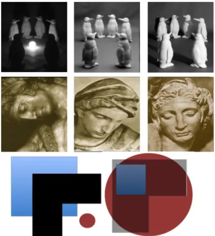
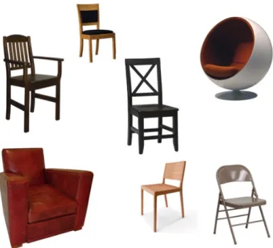
In real life detecting things such as cars and traffic signs in a street image is often a challenging task because of view point variation, difference of object scales or varying illumination conditions (Figure 3). In Figure 4 is shown different instances of the object class chair. Such a large intra-class variation in appearance and shape makes the detection challenging and this is studied in Chapter 3. Other obstacles in object detection are oc-clusion, where the object is partially hidden by some other object and background clutter, where the background of the object can severely affect the detection performance (Figure 5). An ideal system, which output does not depend to these transformations is said to be invariant, such as invariant to rotation or rotation-invariant.

Figure 3. Different objects under illumination change (top), view point variation (middle), and scale change.

(14)

Figure 4.Different instances of the same object category.

(a) (b)

Figure 5. a) Background clutter: A gecko is camouflaged to be part of the tree and thus hard to detect [17]. b) Occlusion: A painting by Réne Magritte where a man face is occluded by an apple.

(15)

1.2 Structure of the thesis

In section 1 we give the reader a general view of computer vision, visual object detection and categorization. After that the thesis has two main parts.

The first part consist of an introduction of well known and efficient detectors and descrip-tors in Chapter 2. Performance of these detecdescrip-tors and descripdescrip-tors in matching task for visual objects classes is studied in Chapter 3. The second part of the thesis starts with de-scription of Bag-of-Features object classification which is described in Chapter 4. Second part ends to an application exploiting Bag-of-Features method in a video scene detection in Chapter 5. A short conclusion of the work done is given in Section 6.

1.3 Goals and restrictions

In the first part, the main goal is to find the best methods for local feature detection and matching. The evaluations is done for local feature detectors and descriptors. The problem is to distinguish instances of the same class and instances from different class from each other. This is a different task such as the wide-baseline matching where the matching is performed for the same objects with different view points. Also for fair comparison of local feature detectors and descriptors, the meta-parameters of different approaches must be configured.

In the second part, the main interest is to develop a novel online video scene boundary detector using local features and Bag-of-Features. The problem is to make a accurate method which detects a cut location between two different scenes, for instance video changing from a ballet to a basketball match, and works in online so that video manip-ulation can be done at the same time while the video is processed. In literature there have been different approaches to solve the problem and some of them have been already successful, but none of them are practical for an online application.

(16)

2 LOCAL FEATURE DETECTORS AND

DESCRIP-TORS

In this section we will briefly introduce the properties of local feature detectors and de-scriptors. We will also give short descriptions of the methods which will be used in Chapter 3 for visual object class matching.

2.1 Introduction

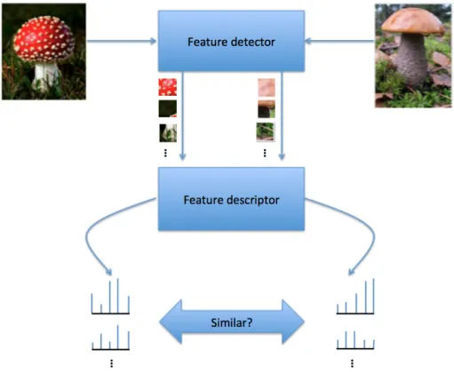
Local feature detectors and their descriptions are the building blocks of many computer vision algorithms. A detector provides detected regions or points for a descriptor which describes them in a certain form. Once we have obtained the features and their descrip-tions from some query image we can compute features from another images and find similar parts between the images (Figure 6). Local descriptors have been used success-fully in many applications such as wide baseline matching [18], object recognition [19], texture recognition [20], robot localization [21], image and video data mining [22], and panoramic photography [16].

(17)

From an image one can extract two kind of low-level features: global features or/and localfeatures. Global features are usually computed from every pixel of the image and they represents the whole image by a single feature element, such as a vector. These kind of features are for example RGB histograms [15] (concerning the colour information of the image) or calculating a Grey Level Co-occurrence Matrix of the image (concerning the textural features of the whole image) [23]. On the other hand local features are computed from multiple locations on the image and as a result we get multiple feature vectors from a single image. One advantage of local features over global features is that they may be used to recognize the object despite significant clutter and occlusion and thus do not require a segmentation of the object from the background unlike many texture features. Advantages of global features are simplicity of the implementation and a compact representation of image features. Combining global and local features we can gain even a 20% boost to performance than using features separately [24]. In this thesis we will now focus on local features.

The terminology in the literature can be sometimes confusing because of the many dif-ferent terms refer to the same thing. In this thesis, we will mainly use local features and keypoints, but also interest points and interest regions are used in the literature. For the descriptors there exists much less variety and often descriptors and descriptions are used. In the thesis, we will use the term local feature descriptors for description of local features.

2.2 Local feature detector properties

Feature detection is a low-level image processing operation which output serves as an in-put for descriptor. Because feature detector is the initial component in the whole pipeline process of object recognition, the overall result will be as good as the feature detector. The detectors can be roughly divided into four different categories: edge detector, cor-ner detector, blob detector, and region detector. In this thesis we are focusing on blob detectors which are discussed in Section 2.4. The detector example images in follow-ing sections are computed usfollow-ing VLFeat toolbox [25] by Andrea Vedaldi in Matlab and OpenCV libraries.

In [13] are listed the following six properties (repeatabilitybeing the most important one) what an ideal local feature has and what a good local feature detector should search:

(18)

trans-formations) the detector should extract the same visual features. Repeatability can be obtained by two ways: either byinvarianceor byrobustness.

• Distinctiveness/informativeness: Different detected features should be discrimina-tive enough so they can be distinguished and matched easily.

• Locality: The features should be local enough to tolerate feature deformation such as occlusion, noise, scale and rotation.

• Quantity: The number of detected features should be large enough, even from on small object. Ideally the number of features should be adjustable by a threshold.

• Accuracy: The properties concerning the detected feature localization (location, scale and shape) should be accurate.

• Efficiency: A faster implementation of a detector is always worth to pursue. In a real-time application it is a crucial property.

In Figure 7 is shown extracted features on the same object in different images. From the images we can see that exactly the same object characteristic features are found despite scale, viewpoint and minor contrast changes.

Figure 7.The detected SURF [26] features on two different images. The yellow lines show which regions match in descriptor space.

(19)

2.3 Local feature descriptor properties

In the previous section we described local features which are used to extract features from an image. After obtaining the features, we have to encode them into mathematical presen-tation which is then suitable for feature matching. The feature needs to be unique i.e. if a similar point is described in two or more images then that point should have similar de-scription. Description or descriptor should have a proper size, a large descriptor will make the computation demanding but if the descriptor is too small then it may not be discrimi-native enough. Descriptors are divided into four classes:Shape descriptors(Contour- and Shape-based),Colour descriptors,Texture descriptorsandMotion descriptors. These can be divided again roughly into family of Histogram of Oriented Gradient (HOG) methods where a histogram is calculated from a patch or binary descriptors where a bit string rep-resents the content of a patch. In this thesis we focus mainly on Texture descriptors and both, HoG and binary descriptors.

An ideal local feature descriptor has the following properties [27]:

• Distinctiveness:Low probability of mismatch.

• Efficiency: Fast to compute.

• Invariance to common deformations: Matches should be found even if several of the common deformations are present: image noise, changes in illumination, scale, rotation and, skew.

2.4 Early work on local features

2.4.1 Hessian detector

Hessian detector proposed by Beaudet et. al [28] in 1978 is one of the first published blob detection algorithms in the literature. Regions detected by the Hessian algorithm are shown in Figure 8. The family of Hessian-based detectors consist of the original Hessian keypoint detector, Hessian-Laplace, and Hessian-Affine. The Hessian detector is based on the2×2HessianmatrixH:

(20)

H= " Lxx(x) Lxy(x) Lxy(x) Lyy(x) # , (1)

where the terms Lxx, Lxy, and Lyy denote the second-order partial derivatives of L(x) at location x = (x, y) i.e., the gradients in the image in different directions. Before we calculate the second order derivatives the image is smoothed by taking the convolution between the imageI and a Gaussian kernel with scaleσ:

L(x) =G(σ)⊗I(x) (2)

To find keypoints, the determinant of the Hessian is computed as:

Det(H) = LxxLyy−L2xy (3)

The determinant of the Hessian matrix is calculated in every pointxin the given image. After obtaining the determinant for every pixel, we search for points where the determi-nant of the Hessian becomes maximal. This is done by using3×3window where the window is swept over the entire image, keeping only pixels whose value is larger than the values of all 8 immediate neighbours inside the window. Then, the detector returns all the remaining locations whose value is higher than a pre-defined threshold valueτ and these will be selected as keypoints.

Figure 8.Local features detected by the original Hessian detector. Note the approach convention to detect features from object contours and corners.

However this approach is not robust to various transformations in the images.The Hessian-Laplaciandetector was introduced to increase robustness and discriminative power of the original Hessian detector. It combines the Hessian operator’s specificity for corner-like

(21)

structures with the scale selection mechanism presented by Lindeberg [29]. The Linde-berg mechanism searches for scale space extrema of a scale-normalized Laplacian-of-Gaussian(LoG):

S =σ2(Lxx+Lyy), (4)

whereσ2 _{is the scale factor. In the Hessian-Laplacian method we build separate spaces} for the Hessian functions and the Laplacian. Then we use Hessian to detect candidate points from different scale levels and select those candidates to our keypoints which the Laplacian simultaneously attains an extremum over scale. Now, the obtained keypoints will be robust to changes in scale, image rotation, illumination and camera noise.

To achieve invariance against viewpoint changes an extended version of Harris-Laplacian have been pronounced: Hessian-Affinedetector [30, 31]. First, we use the scale-invariant Hessian to find initial keypoints and estimate the shape of the region with the second moment matrixM: M=G(σ) " L2_x(x) LxLy(x) LxLy(x) L2y(x) # , (5)

where we can compute the eigenvaluesλ1 andλ2 by the following equations:

Tr(M) = λ1+λ2, (6)

Det(M) =λ1λ2. (7)

The obtained eigenvalues from Equations 6 and 7 gives us an elliptical shaped region, cor-responding to a local affine deformation. The elliptical shape is normalized to circular one and the point location and scale is recovered. Again the moment matrix is calculated from the normalized region and this process is iteratively continued until the the eigenvalues of the matrix are equal.

2.4.2 SIFT detector and descriptor

The SIFT (Scale-Invariant Feature Transform) detector was first introduced by David Lowe in 1999 [8] and later improved in 2004 [32]. In contrast to Harris [6] method where corners are localized when there is low auto-correlation in all direction, SIFT lo-calizes features where there are "blob-like" structures in the image. Lowe aimed to create a detector which would be a invariant to translation, rotation and scale. The SIFT al-gorithm builds a scale-space representation of the original image. This is achieved by a Difference of Gaussian (DoG) approach combined with interpolation over the scale-space

(22)

which leads to the locations of stable keypoints in that scale-space representation of the image. After the localization, each keypoint is assigned an orientation, which leads to the desired rotation invariance. Below are listed the key steps in SIFT algorithm:

1. Scale-space extrema detection: Image is convoluted with Gaussian filters on differ-ent scales and then the difference of successive Gaussian-blurred images are taken. This is called Difference of Gaussians (DoG) can be written as:

D(x, σ) =L(x, kiσ)−L(x, kjσ), (8) whereL(x, kkσ) is the convolution of the original image I(x)with Gaussian blur G(x, kkσ)at scalekkσ. Once we have obtained DoG images, keypoint candidates are identified as local minima/maxima of the DoG images over all scales.

2. Keypoint localization: After the scale-space extrema detection we have gathered lots of keypoint candidates and we have to perform an eliminations of the unstable keypoints. A detailed fit to nearby data is performed to determine location, scale, and ratio of principle curvatures. In Lowe’s first method the keypoints accurate position and scale of a central sample point was acquired. In more recent work, the author fit a 3D quadratic function to improve interpolation accuracy. In addition, the Hessian matrix was used to eliminate edge responses with poorly determined locations.

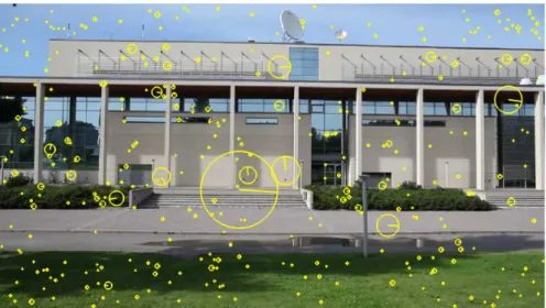
3. Orientation assignment: In this step we achieve rotation-invariance by assigning to each keypoint one or more orientations based on local image gradient directions. We create a histogram of local gradient directions at selected scale. Histogram is then smoothed by every sample’s gradient magnitude and by a Gaussian weighted circular window. Finally canonical orientation is assigned at peak of smoothed histogram where each key specifies stable 2 dimensional coordinates. In Figure 10 is shown detected SIFT features with the orientation.

The SIFT keypoint descriptor computation is shown in Figure 9. The left image of the figure with small arrows represents the gradient magnitude and orientations at each sam-ple locations. The circle around the samsam-ples is a Gaussian weighting function. It is used to weight the gradient magnitudes of each sample point in a way that it gives less em-phasis to gradients that are far from the center of descriptor. The right part of the figure represents the2×2descriptor matrix of the8×8neighborhood. Every cell in the matrix contains accumulated gradients to 8 directions from the corresponding4×4subregions.

(23)

However, the best results are typically achieved with4×4descriptor matrix with 8 orien-tations [32]. In this case our descriptor has4×4×8 = 128dimension in total. Finally the descriptor vector is normalized to enhance invariance to affine changes in illumination.

Figure 9.A2×2SIFT descriptor (right) computed from8×8sample neighbourhood (left).

Figure 10.Detected SIFT features and their orientations.

2.4.3 Dense sampling

Dense sampling is one of the most commonly used low-level image representation method, which uses a fixed pixel interval (horizontally and vertically) between sample points i.e., points are sampled on a regular dense grid. The chosen length of the interval between sample points determines the number of patches to be sampled from the image. The in-terval is usually set that different patches are overlapping 50% [33]. Keeping the inin-terval

(24)

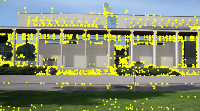
value same for same size images the "detector" generates constant amount of samples de-spite for instance contrast shifts and thus dense sampling on a regular grid results in a good coverage of the entire object or scene. Other benefit of dense sampling is a regular spatial relationship between sampled patches where as local feature detectors find interest points only from specific locations (corners, blobs, etc.) which makes it hard to model spatial configuration of features (for instance the spatial relationship between eyes and mouth on human face). However, dense sampling cannot reach the same level of repeatability as local features do. In [34] it is shown that dense sampling outperforms local features on Bag-of-Words based classification. In Figure 11 is illustrated the sampled patches having 50 pixel distance to each other.

Figure 11.Dense sampling.

2.5 More recent and efficient implementations

2.5.1 BRIEF descriptor

BRIEF (Binary Robust Independent Elementary Features) was one of the first published binary descriptor by Calonderet al. [35]. Binary descriptors try to provide an alternative method to the widely used floating point descriptors such as SIFT. BRIEF was originally made to beat SURF [26] and U-SURF (upright version of SURF) descriptors on recogni-tion performance, while only using a fracrecogni-tion of the time required by either. BRIEF can produce a very good results with only 256 bits, or even 128 bits, which is a significant

(25)

advantage when millions of descriptors must be stored.

The approach main assumption is that image patches could be effectively classified on the basis of a relatively small number of pairwise intensity comparisons. The descriptors are binary strings where each bit represents a simple comparison between two points inside a patch. Before the binary tests we have to first smooth the patch using the Gaussian kernel of sizeσ. More precisely, we can define testτ on pathPof sizeS×Sas

τ(P;x,y) :=    1 ifP(x) <P(y) 0 otherwise (9)

whereP(x) is the pixel intensity in a smoothed version of Pat x= (u,v)T. The BRIEF descriptor is defined as a vector ofnbinary test:

fn(P) :=

X 1≤i≤n

2i−1τ(p;x, y) (10)

where a typical value for nis 128, 256 or 512 [35]. The only properties that have to be taken account when creating the descriptors are the kernels which are used to smooth the patches and the spatial arrangement of the (x,y)-pairs.

Smoothing of the patches is a necessary step in the process of obtaining the BRIEF de-scriptors. BRIEF is highly sensitive to noise due method’s pixel-to-pixel test protocol. To make approach more robust and increase the stability and the repeatability different smoothing kernel sizes were studied by Calonderet al. [35]. They found out that a prac-tical value for Gaussian kernel was 2. Spatial arrangement of the binary tests were their second experimented parameter. They tested five different sampling geometries, where the Uniform (−S

2,

S

2) and the Gaussian S(0, 1 25S

2₎ _(S _{was the size of the image patch)} distributions were the best methods.

The authors reported the performance results of BRIEF against OpenCV implementation of SURF. The performance rate histograms were almost superposed and there were no significant differences in any categories. The speed comparison showed clear differences among methods and BRIEF was 35- to 41- fold faster building descriptors over SURF where the time for performing and storing the tests remains virtually constant. For match-ing the speed-up was 4- to 13-fold. U-SURF computation time was between these two, but still far away from the BRIEF results. However, BRIEF does not tolerate well orien-tation and roorien-tation and with a bigger test set of different objects it might not compete with SIFT and SURF as it was noted by the authors.

(26)

2.5.2 ORB detector

ORB (Oriented FAST and Rotated BRIEF) is a fast local feature detector first introduced by Ethan Rublee, Vincent Rabaud, Kurt Konolige and Gary Bradski [36]. ORB is one of the most efficient detector algorithm in the field of image processing [37] and it is based on FAST (Features from Accelerated Segment Test) keypoint. ORB can also be used to compute the visual descriptors and the approach is based on a steered version of BRIEF with an additional learning step. The authors main idea was to develop a method which is a computationally-efficient replacement to SIFT that has similar matching performance, is less affected by image noise, and is capable of being used for real-time performance. ORB starts the search of local features by FAST corner detector. It is a computationally efficient and produces high quality features. After we have retrieved the features we apply a Harris corner measure to find the top N features among them. We apply also a scale pyramid to get multiscale-features. However, the FAST does not compute the orientation so we do not have rotation-invariant features yet. Authors decided to use Rosin’s [38] orientation measure, theintensity centroid, to include rotation invariance. First we define the moments of a patch as:

mpq =

X

x,y

xpyqI(x, y), (11)

and centroid can be determined as

C= (m10

m00 ,m01

m00

). (12)

The corner orientation is then the angle of the vector−→OC, whereOis the corner’s center. The orientation is simply calculated as:

θ=atan2(m01, m10), (13)

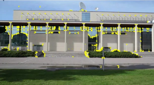
where atan2 is the quadrant-aware version of arctan. To improve the rotation invariance of this measure one should computexandyremaining within a circular region of radius r, wherer is the size of the patch. Below (Figure 12) are shown the detected features by ORB detector.

(27)

(28)

3 COMPARISON OF FEATURE DETECTORS AND

DESCRIPTORS FOR VISUAL OBJECT CLASS

MATCHING

In Chapter 2 we presented local feature detectors and descriptors which are used in many computer vision problems such as panorama image stitching [16], robot localization [39], and wide baseline matching [18]. In all these cases, the feature correspondences are needed to match several views of the same scene. Local feature detectors and descriptors performance for these kind of problems have been already well covered by Mikolajczyk [30], Mikolajczyk and Schmid [27] and in the more recent paper [37] by Miksik and Mikolajczyk. Another interesting application would be to match two views of different objects from the same class. For instance we want to classify a mountain bicycle and a trial bike to be related because they are both from the same class bicycle. Although both are objects from the same class, their visual appearance can be very different, and thus, the original evaluation of detectors and descriptors are not directly applicable.

Various methods have been proposed for detecting interest points/regions and to construct descriptors from them, most of which are designed with a different applications in mind. In [30, 27] and [37] the authors evaluated and compared the most popular and recent de-tectors and descriptors. The detector were evaluated by their repeatability rations and total number of correspondences over several views of scenes and with various imaging dis-tortion types. The descriptors were evaluated by their matching rates for the same views. Comparisons concerning object classification tasks were reported in [20] and [19], but in these works the evaluation was tied to a single methodological approach, namely vi-sual Bag-of-Words (BoW). Moreover, many fast descriptors have been proposed recently: SURF [26], FREAK [40], ORB [36], BRISK [41], BRIEF [35]

In this chapter we will extend the original detector and descriptor benchmarks in [30, 27] to intra-class repeatability and matching. We evaluate the popular and efficient detectors and descriptors and their various implementations with the proposed framework. The detectors repeatability rates and the total number of correspondences for different objects from the same class were evaluated over 750 image pairs from different image databases. The descriptors were evaluated by their matching rate for the same data set. In addition, we investigate the effect of using multiple best matches(K = 1,2, ...)and introduce an alternative performance measure: match coverage.

(29)

3.1 Previous work

The evaluation method described in this chapter is basically an extension of the evaluation framework from [30, 27]. The benchmark framework provides a fair way to compare detectors and descriptors by evaluating the overlap of the detected areas of interest as well as how well these regions actually match. We will follow the same evaluation principles as in the framework in our experiments: repeatabilityfor detectors andmatch count/ratio for descriptors. Most of the results are included to the recent paper [42].

We refer to these repeating and matching regions as "category-specific landmarks". A qualitative measure to visualise descriptors "(HOGgles)" was recently proposed by Von-dricket al. [43], but its main use is in image-wise debugging of existing methods. More quantitative evaluations were reported by Zhanget al. [20] and Mikolajczyk et al. [19], but these were quite heuristic and tied to a single methodology, the visual Bag-of-Words (BoW) [10, 9]. In this work, we show that the original evaluation principles can be adopted to obtain similar quantitative performance measures in general, comparable and intuitive forms used in the original works of Mikolajczyket al., and not tied to any specific approach.

3.2 Performance measurement protocol

We believe that the general evaluation principles in [30, 27] hold also in the visual object categorization context:

1. Detectors which return the same object regions for class examples are good detec-tors –detection repeatability.

2. Descriptors which match the same object regions between class examples are good descriptors –match count/ratio.

For detectors thedetector repeatability rateis the most important value to measure perfor-mance of a detector [13]. We start the calculations by comparing all the detected regions in two image pairs. If theoverlap erroris smaller than0 then two regions are deemed to correspond:

1− Rµα ∩R(HTµbH)

Rµα ∪R(HTµbH)

(30)

where Rµ represents the detected elliptic region defined by xTµx = 1 and H is the homography relating the two images. Before calculating the overlap error we have to normalize the corresponding areas. This is done because the bigger the ellipses are, the smaller is the overlap error in the measurement and vice versa ( Figure 13). To compensate

Figure 13.Size of the ellipses have an effect on the overlap measurement [30].

for the effect of regions of different sizes, Mikolajczyk determined the scale factor that transforms reference image into a region of normalized size (in the experiments normal-ized to a radius of 30 pixels). After that, we apply the determined scale factor to both the region in the reference image and the region detected in the other image which has been mapped onto the reference image by an estimated unknown affine homography. Now, the actual overlap error as stated in Equation 14, can be computed. In Mikolajczyk exper-iment the overlap error was set to 40%. After we have obtained all the correspondence regions, we can calculate therepeatability rateas:

repeatability rate = #of correspondences

min(#of reg in img A,#of reg in img B) ∗100 (15)

Taking the minimum of detected regions in imageAandB we will only include regions that are found in both images.

As we stated earlier a good descriptor should be discriminative to match only correct regions and also it should be robust to some small appearance variations between the ex-amples. The descriptor performance were obtained in the Mikolajczyk and Schmid paper [27] by computing statistics of the correct and false matches. Our descriptor performance

(31)

will be evaluated by the average number of matches and the median number of matches. In our work descriptors results are expected to be weaker due to increased appearance variance. For instance, scooter and road bikes are both found in the Caltech-101 motor-bike category, but their pair-wise similarity is much weaker than between two scooters or two road bikes.

3.3 Data

Both detectors and descriptors were evaluated using three different image databases: Caltech-101 [44], R-Caltech-101 [45] and ImageNet [46]. Caltech-101 image database contains images and annotations for bounding boxes and outlines enclosing each object. We chose Caltech-101 because it is popular in papers related to object categorization and contains rather easy images for benchmarking. We selected ten different classes from the database to get good view of the performance over different content. Every image is scaled not to exceed 300 pixels in width and height. The classes are watch, stop_sign, starfish, revolver, euphonium, dollar_bill, car_side, air planes, Motorbikes andFaces_easy.

The Caltech 101 database however has some weaknesses: the objects are practically in a standard pose and scale in the middle of the images and background varies too little in certain categories making it more discriminative than the foreground objects. To make our benchmark process more challenging we will use the randomized version of the Caltech-101 database where we use the same classes but with randomized background, object orientation and locations. Annotations for bounding boxes and outlines are provided. To experiment our detectors and descriptors with more recent images, we chose to in-clude ImageNet image dataset to our evaluation. ImageNet provides over 100,000 dif-ferent meaningful concepts and millions of images. However, bounding boxes, outline coordinates, and landmarks for the objects were not provided and we had to mark them manually. We selected Watch, Sunflower, Pistol, Guitar, Elephant, Camera, Boot, Bird andAeroplaneobject categories to be in our testing process.

(32)

3.4 Comparing detectors

3.4.1 Annotated bounding boxes and contour points

In our experiment annotations for object bounding boxes and contour points are given for each images. Box coordinates are given as vector of 4 elements describing the top left and bottom right corner of the box. The outlines of objects for Caltech-101 and ImageNet image set are 2×n matrices containing n(x, y)-pairs for contour points. Since we are only interest of benchmarking how well detected features found from the objects match to different object from the same category, detected features outside the object contour are discarded. With more challenging randomized Caltech-101 we only used bounding boxes so some background features around the objects will be detected. In Figure 14 is shown the bounding box and the contour of an image from Caltech-101 dataset, all the detected SIFT features and the remaining ones after the elimination process.

3.4.2 Annotated landmarks and affine transform

For every image there are manually annotated landmarks (5-12 landmarks per category) which are marked to the sample image locations, which are semantically similar between the same category images. By these landmarks and estimating the pair-wise image trans-formations using the direct linear transform [47] we can establish affine correspondence between image pairs. In Figure 15 is shown two examples of landmark locations on an object and how well they match with other object’s landmarks.

3.4.3 Selected local feature detectors

The detectors for the experiment were selected from the earlier study [48] where the performance of different detectors and descriptors were evaluated. Detector evaluations included nine publicly available detectors:

1. Detectors from Zhao’s Lip-vireo toolkit1_{: difference of Gaussian (}_dog-vireo_), Lapla-cian of Gaussian (log-vireo) and Hessian affine (hesslap-vireo).

2. Three implementations by Mikolajczyk2_{: Hessian-affine detectors (}_hessaff_{) and}

1_{http://code.google.com/p/lip-vireo} 2_{http://featurespace.org}

(33)

(a)

(b) (c)

Figure 14. Elimination of the features outside the object: a) the bounding box (yellow line) and the contour (red line) of the face, (b) the detected SIFT features, and c) the remaining features after elimination.

(hessaff-alt) and Speeded-up robust feature detector (surf).

3. Two detectors from VLFeat toolbox3: Maximally stable extremal regions (mser) and SIFT (sift).

The results indicated thathesslap-vireo,dog-vireoandsurf were the best detectors based on the repeatability rate which was over30%with all the methods. However, the hesslap-vireo provided much more correspondences (57) on average compared to for instance the highest repeatability rate (30%)dog-vireowhich had 16 average on correspondences. Considering the repeatability rate and the average correspondences equally the best detec-tors werehesslap-vireo(30.6%, 57.4),hesaff (25.4%, 47.8)andlog-vireo(26.3%, 46.5).

(34)

(a) (b)

(c) (d) Subfigure 3 caption

Figure 15.Two objects from different classes with annotated landmarks (the leftmost images) and 50 examples (affine) projected into a single space (denoted by the yellow tags).

In this thesis, we report the results for the hesaff detector (hesaff) and VLFeat implemen-tation of SIFT.

In additions to these we were interested to evaluate some of the more recent and efficient detectors from [37]: BRIEF [35], BRISK [41] and ORB [36]. The best results were obtained using the ORB OpenCV implementation 4 which results are reported in this thesis. Moreover, dense sampling has replaced detectors in the top methods (Pascal VOC 2011 [49]) and we added the dense SIFT in VLFeat toolbox to our evaluations (dense).

3.4.4 Performance measures and evaluation

For the detector performance evaluation, the test protocol is similar to Mikolajczyk bench-mark [30] which main points were discussed in section 3.2. Because we are focusing on

(35)

object matching more than a general feature similarity measurement, we will make an exception to the protocol that only interest points inside the contour will be selected. For each image pair, points from the first image are projected onto the second image by the affine transformation estimated using the the annotated landmarks described in the sec-tion 3.4.2. The interest points (regions) are described by 2D ellipses and if a transformed ellipse overlaps with an ellipse in the second image (more than a selected threshold value) a correct correspondence is recorded. The reported performance numbers are the average number of corresponding regions between image pairs and the total number of detected regions. The detector performs well if the total number of detected regions is high and most of them overlap with the second image corresponding regions. We adopt the pa-rameter setting from [30]: 40% overlap threshold and normalization of the ellipses to the radius of 30 pixels. The normalization is required since the overlap area depends on the size of the ellipses. The algorithm for evaluating detectors is shown below:

Algorithm 1The detector benchmark procedure 1: for allimage pairsdo

2: Extract local features

3: Use foreground masks to filter out features outside the object 4: Compute the true transformation matrixHfor image pairs 5: Transform all detected regions onto the second image usingH 6: for allregionsdo

7: if Overlap is more than a threshold t with some of the regions in the other imagethen

8: Increment the correspondency scoreci

9: end if

10: end for

11: Calculate the repeatability raterj usingci

12: end for

13: Return the correspondencescand repeatabilitiesr

3.4.5 Results

It is noteworthy that this evaluation differs from the earlier studies [48] in the sense that in-stead of using the default parameters for each detector we adjusted their meta-parameters to return on average 300 regions for each image. This makes the evaluation fair for all the detectors because of the number of detected regions will surely have an effect to num-ber of correspondences between image pairs. The adjustment of the meta-parameters is discussed more in section 3.4.6. The results of the detector experiment are reported in Table 2 and Figure 16. From the results we can see that the starfish and the revolver

(36)

categories were the hardest ones for all the detectors. Performance of dense sampling in Faces_easycategory is very good: it provides a lot of correspondence regions compared to other methods and the same regions are mostly found in both images.

With the adjusted meta-parameters the difference between the detectors is less significant than in the earlier evaluation [48] and the previous winner, Hessian-affine, is now the weakest. With the default parameters Hessian-affine returns almost five times more fea-tures than for instance SIFT, which made the evaluations too biased against the other de-tectors. The original SIFT detector performance without the parameter adjustment would be by order of magnitude worse. The new winner in the detector benchmark is clearly the dense sampling with a clear margin to the next best detector ORB. However, when computational time is crucial, the ORB detector seems attempting due to its speed.

Table 2.The Overall result table of detector evaluation. Detector Avg # of corr. Avg. rep. rate

vl_sift 127.5 41.6%

fs_hessaff 79.3 26.0%

cv_orb 132.0 43.5%

vl_dense 192.3 64.6%

3.4.6 Detecting more regions

In the previous section, we adjusted detector meta-parameters to return on average 300 regions for each image. That made detectors produce very similar results while using the default parameters in our previous work lead to completely different interpretation. It is interesting to study whether we can exploit meta-parameters further to increase the number of corresponding regions. For ORB we adjusted the edge threshold, for Hessian-affine the feature density and the Hessian threshold, for SIFT the number of levels per octave, and for the dense the grid step size. We computed the detector repeatability rates as the functions of the number of detection regions and the results are reported in Fig-ure 17. FigFig-ure also shows the number of returned regions by default parameters with the black dots. As expected the meta-parameters have almost no effect to the dense detection while Hessian-affine, ORB and especially SIFT clearly improve as the number of the re-gions increase (SIFT rere-gions saturate to the same locations approximately at 600 detected regions). For the most difficult classes (starfishandrevolver) the performance of the de-tectors could be increased by a iterative search of the optimal parameters but this could

(37)

(a)

(b)

Figure 16. Detector evaluation in object class matching. Meta-parameters were set to return on average 300 regions. (a) average number of corresponding regions and (b) repeatability rates.

(38)

compromise the performance of other category classes.

Figure 17. Detector repeatability as the function of the number of detected regions adjusted by the meta-parameters

3.5 Comparing descriptors

A good region descriptor for object matching should be discriminative to match only cor-rect regions, and also tolerate small appearance variation between the examples. These are general requirements for feature extraction in computer vision and image process-ing. The descriptor performance were obtained in the original work [27] by computing statistics of the correct and false matches. Between different class examples, descriptor matches are expected to be weaker due to increased appearance variation.

3.5.1 Available descriptors

In this experiment we used detector-descriptor pairs. The earlier studies included the following detector-descriptors combinations:

(39)

2. Hessian-affine and steerable filters

3. Vireo implementation of Hessian-affine and SIFT 4. Original SIFT detector and SIFT descriptor

5. Alternative (Vireo) implementation of SIFT and SIFT 6. SURF and SURF

Within their default parameters the combinations 1) and 2) utilizing Mikolajczyk’s im-plementation of Hessian-affine detector were clearly superior to other methods [48], but here we adjust the same meta-parameters as described in section 3.4.6 to return the same average number of regions (300).

To these experiments, we also include the best fast detector-descriptor pair: ORB and BRIEF. The following combinations will be reported: vl_sift+vl_sift (FeatureSpace im-plementation), fs_hessaff+fs_sift (FeatureSpace implementation), cv_orb+cv_brief (OpenCV implementation), cv_orb+cv_sift (OpenCV, to compare SIFT and BRIEF), vl_dense+vl_sift(VLFeat implementation). It should be noted that available descriptors are not guaranteed to work well with different implementations of detectors. Thus we will use in our evaluation pair-wise detector-descriptor combinations only. Because the cho-sen detector has also impact on the performance of the descriptor, we wanted to testvl_sift descriptor with two different detectors. We also tested the RootSIFT descriptor from [50] which should lead to performance boost of SIFT by using a square root (Hellinger) kernel instead of the standard Euclidean distance. In their experiment this led to a notable per-formance increase but in our case it provided insignificant difference to the original SIFT (mean: 3.9→4.2, median: 1→1).

3.5.2 Performance measures and evaluation

In the earlier work [48] they used a simplified version of the Mikolajczyk’s descriptor performance measure: the ellipse overlap was replaced by normalized centroid distance of the matching regions. However, the results by the simplified rule turned out to be too optimistic and in this work we adopt the original measure.

The rule is the same as with the detectors, if the best matching regions have sufficient over-lap the match is correct. Descriptors are computed for all detected regions (foreground only). Images are processed pair-wise and the best match for each region is selected from the full distance matrix. It is worth noting that the rule proposed in [32] for discarding "bad regions" (ratio between the first and the second best is less than 1.5) is not used

(40)

Algorithm 2Descriptor performance evaluation procedure 1: for allimage pairsdo

2: Extract local features

3: Use foreground masks to filter out features outside the object 4: Compute the true transformation matrixHfor image pair 5: Transform all detected regions onto the second image usingH 6: for allregionsdo

7: Find theN closest descriptors associated with the region 8: ifregion overlap is more than a thresholdtthen

9: Increase the number of matches formi

10: end if

11: end for 12: end for

13: Return the total number of matchesm

since it results complete failure. We used the default ellipse overlap threshold 50% from [27] which is little bit looser than in detector evaluation, but also more strict threshold were tested. Our performance numbers are the average number of matches and median number of matches. In [27] recall versus 1-precision was used for quantitative evalua-tion of descriptor matching. Our case however is different to the wide baseline matching where image pairs are tested one by one. We decided to report the average number of matches that is more compact and intuitive for a large set of image pairs containing cat-egory instances and the average numbers of matches were also reported by Mikolajczyk and Schmid. The Algorithm 2 also provides an alternative measure,coverage, which mea-sures the number of images "covered" with at least the given number of correspondences N (coverage N). In the detector evaluation the mean and median numbers were almost the same, but here we report the both since for the descriptors there is significant discrepancy between the mean and median numbers.

3.5.3 Results

The average number of matches for the descriptor evaluation is shown in Figure 18 and the overall results including the median, the results for more strict overlap, and compu-tation time are reported in Table 3. For many classes, the mean and median numbers are very low, and for instance the starfish category is extremely hard for every descriptor. However, with dense grid sampling coupled with SIFT we get decent results for most of the categories and its performance is superior compared to all other descriptors, achiev-ing the average of 23.0% matches per class and median of 10.0% matches. The second best descriptor is FeatureSpace implementation of fs_hessaf+fs_sift and the rest of the

(41)

descriptors are near behind with minor performance decrease. The more strict overlaps, 60% and 70%, provide almost the same numbers verifying that the matched regions do match well also spatially.

Figure 18. The average number of matches per class in descriptor evaluation when using the default threshold overlap 50%.

Table 3.Overall result table of description evaluation. The default overlap threshold is 50% [27], 60% and 70% results demonstrate the effect of the more strict overlaps. The computation time are average detector and descriptor computation times for one image pair.

Detector+descriptor Avg # Med # Avg # (60%) (70%) Comp. time (s.)

vl_sift+vl_sift 3.9 1 2.8 1.6 0.15

fs_hessaff+fs_sift 6.5 2 5.9 4.9 0.22

vl_dense+vl_sift 23.0 10 22.3 20.2 0.76

cv_orb+cv_brief 3.0 1 2.9 2.7 0.11

cv_orb+cv_sift 5.4 2 4.8 4.1 0.37

The best results were obtained for the stop signs, dollar bills and faces, but the overall performance is poor. The best discriminative methods could still learn to detect these

(42)

categories, but it is difficult to imagine naturally emerging "common codes" for other classes except the three easiest. It is surprising that the best detectors, Hessian-affine and dense sampling, were able to provide 79 and 192 repeatable regions on average, but only roughly 10% of these match in the descriptor space. Despite the fact that the SIFT detector performed well in the detector experiment, its region do not match well in this experiment. The main conclusion is that the descriptors that are developed for wide baseline matching do not work well in the matching regions between different class examples.

3.5.4 The more the merrier

Similar to Section 3.4.6 we studied how the average number of matches behaves as the function of the number extracted regions. This is justified as some work [34] claim that the number of interest points extracted from the test images is the single most influential parameter governing the performance. The result graph is shown in Figure 19.

Figure 19. Descriptors’ matches as function of the number of detected regions controlled by the meta-parameters (default values denoted by black dots).

The results show that adding more regions by adjusting the detector meta-parameters provides only minor improvement to the average number of matches. Clearly, the "best

(43)

regions" are provided first and the dense sampling performs much better indicating that what is "interesting" for the detector is not necessarily a good object part.

3.6 Advanced analysis

In this section, we address the open questions raised during the detector and descriptor comparisons in Section 3.4 and 3.5. The important questions are: why only a few matches are found between different class examples and what can be done to improve that? Why dense sampling outperforms all interest point detectors and does it have any drawbacks? Do our results generalize to other data sets.

3.6.1 ImageNet classes

To validate our results, we selected 10 different categories from the state-of-the-art object detection database: ImageNet [46]. The configuration set up was the same as in the section 3.5: the images were scaled to the same size as the Caltech-101 images, the foreground areas were annotated and the same overlap threshold values were tested. The results for the ImageNet classes are reported in Figure 20 and overall results in Table 4. The average number of matches is roughly half of the number of matches with Caltech-101 images which can be explained by the fact that the data set is more challenging due to 3D view point changes. However, the ranking of the methods is almost the same: dense sampling and SIFT is the best combination and the SIFT detector and descriptor pair is the worst. The results validate our findings with Caltech-101.

Table 4.Overall result table of description evaluation using ImageNet dataset. The default overlap threshold is 50% [27], 60% and 70% results demonstrated the effect of the more strict overlaps.

Detector+descriptor Avg # Med # Avg # (60%) (70%)

vl_sift+vl_sift 1.2 0 0.7 0.3

fs_hessaff+fs_sift 3.4 2 2.8 1.9

vl_dense+vl_sift 12.4 7 11.6 10.2

cv_orb+cv_brief 2.2 1 1.9 1.5

(44)

Figure 20.Average number of matches per class using ImageNet database images (overlap thresh-old 50%).

3.6.2 Beyond the single best match

In object matching, assigning each descriptor to several best matches, "soft assignment" [51, 52, 53], provides improvement and we want to experimentally verify this finding using our framework. The hypothesis is that the best matches in descriptor space are not always correct between two image pairs, and thus, not only the best, but a few best matches can be used. This was tested by counting matches as correct if they were within theKbest and the overlap error was under the threshold. To measure the effect of multiple assignments, we establish a new performance measure: coverage. Coverage corresponds to the number of image pairs for which at least N matches have been found (coverage-N) and this measure is more meaningful than the average number of matches since there was strong discrepancies between the average and median numbers. We tested the multiple assignment procedure by accumulating matches overn = 1,2, ..., K best matches. The corresponding coverage forK = 1,5,10are shown in Figure 21 and Table 5. Obviously, more image pairs contain at leastN = 5 thanN = 10matches. With K = 1(only the

(45)

Table 5. Average number of image pairs for whichN = 5,10 matches were found usingK = 1,5,10nearest neighbors. Coverage-(N = 5) Coverage-(N = 10) Detector+descriptor K=1 K=5 K=10 K=1 K=5 K=10 cv_orb+cv_sift 7.9 16.7 23.0 3.6 11.1 15.7 vl_dense+vl_sift 16.0 19.5 19.8 12.9 18.1 19.6 cv_orb+cv_brief 4.5 13.3 17.9 2.1 9.5 13.2 fs_hesaff+fs_sift 7.3 17.9 20.4 3.5 12.7 17.7 vl_sift+vl_sift 4.3 8.0 11.3 2.5 4.3 6.0

best match) the best method, VLFeat dense SIFT, finds at leastN = 5matches in 16 out of 25 image pairs and 13 for N = 10. When the number of best matches is increased to K = 5, the same numbers are 19 and 18, respectively, showing clear improvement. BeyondK = 5the positive effect diminishes and also the difference between the methods is less significant.

3.6.3 Different implementations of the dense SIFT

During the course of work, we noticed that different implementations of the same method provided slightly different results. Since there are two popular implementations of dense sampling with the SIFT descriptor, OpenCV and VLFeat (two options: slow and fast), we compared them. The result corresponding to the previous experiments in section 3.5 are shown in Figure 22. There are slight differences in class results due to implementation differences, but the overall performances are almost equal. However, the computation time of the VLFeat implementation is much smaller compared to the OpenCV. In addition, the VLFeat fast version is roughly six times faster than the slower version of SIFT.

3.6.4 Challenging dense sampling: r-Caltech-101

With dense sampling the main concern is its robustness to changes in scale and, in partic-ular, orientation, since these are not estimated similar to interest point detection methods. In this experiment, we replicated the previous experiments with the two dense sampling implementations and the best interest point detection method using the randomized ver-sion of the Caltech-101 data set: r-Caltech-101 [45]. R-Caltech-101 contains the same objects (foreground), but with varying random Google backgrounds and the objects have been translated, rotated and scaled randomly. These are illustrated in Figure 23. An

(46)

ex-Figure 21. Number of image pairs for which at least N = 5,10 (left column, right column) descriptor matches were found (Coverage-N).K = 1,5,10denotes the number of best matches (nearest neighbours) counted in matching (top-down).

(47)

Figure 22.Average number of matches per class using ImageNet database images (overlap thresh-old 50%) and different dense SIFT implementations.

ception to the previous experiments is that we discard features outside the bounding boxes instead of using the more detailed object contour. The detector and descriptor results of this experiment are reported in Figure 24. Now it is clear that artificial rotations affect to the dense descriptors while Hessian-affine is unaffected (actually improves). It is note-worthy that the generated pose changes in r-Caltech-101 are rather small ([−20◦,+20◦]) and the performance drop could be more dramatic with larger variation. An intriguing research direction is detection of scaling and rotation invariant dense interest points.

3.7 Discussion

In this chapter, the well accepted and highly cited interest point detector and descriptor performance measures by Mikolajczyk et. al[30, 27], the repeatability and number of matches, were extended to measure intra-class performance with visual object categories. The most popular state-of-the-art and more recent efficient detectors and descriptors were compared using the Caltech-101, r-Caltech-101 and ImageNet image datasets. Interest points and regions have been the low-level features in visual class detection and