Structure and asymptotic theory for nonlinear models with GARCH errors

Availableonlineatwww.sciencedirect.com

ScienceDirect

HOSTED BY

EconomiA16(2015)1–21

Structure

and

asymptotic

theory

for

nonlinear

models

with

GARCH

errors

夽

Estrutura

e

Teoria

Assintótica

para

Modelos

Não-lineares

com

Erros

GARCH

economia

e

financ¸as

Felix

Chan

a

,

Michael

McAleer

b,c

,

Marcelo

C.

Medeiros

d,∗

a_{SchoolofEconomicsandFinance,CurtinUniversityofTechnology,Australia} b_{DepartmentofQuantitativeFinance,NationalTsingHuaUniversity,Taiwan}

c_{EconometricInstitute,ErasmusUniversityRotterdam,TheNetherlands} d_{DepartmentofEconomics,PontificalCatholicUniversityofRiodeJaneiro,}

Brazil

Received3June2014;receivedinrevisedform7January2015;accepted22January2015 Availableonline7February2015

Abstract

Nonlineartimeseriesmodels,especiallythosewithregime-switchingand/orconditionallyheteroskedasticerrors,havebecome increasinglypopularintheeconomicsandfinanceliterature.However,muchoftheresearchhasconcentratedontheempirical applicationsofvariousmodels,withlittletheoreticalorstatisticalanalysisassociatedwiththestructureoftheprocessesorthe associatedasymptotictheory.Inthispaper,wederivesufficientconditionsforstrictstationarityandergodicityofthreedifferent specificationsofthefirst-ordersmoothtransitionautoregressionswithheteroskedasticerrors.Thisisessential,amongotherreasons, toestablishtheconditionsunderwhichthetraditionalLMlinearitytestsbasedonTaylorexpansionsarevalid.Wealsoprovide sufficientconditionsforconsistencyandasymptoticnormalityoftheQuasi-MaximumLikelihoodEstimatorforageneralnonlinear conditionalmeanmodelwithfirst-orderGARCHerrors.

©2015NationalAssociationofPostgraduateCentersinEconomics,ANPEC.ProductionandhostingbyElsevierB.V.Allrights reserved.

JELclassification: C22

Keywords: Nonlineartimeseries;Regime-switching;Smoothtransition;STAR;GARCH;Asymptotictheory

夽 _{Thispaperwascirculatedpreviouslyas“StructureandAsymptoticTheoryforSTAR-GARCH(1,1)Models”.TheauthorswishtothankThierry}

Jeantheau,OfferLieberman,ShiqingLing,HowellTongandAlvaroVeigaforinsightfuldiscussions.Thefirstauthoracknowledgesthefinancial supportoftheAustralianResearchCouncil,thesecondauthorismostgratefulforthefinancialsupportoftheAustralianResearchCouncil,National ScienceCouncil,Taiwan,andtheJapanSocietyforthePromotionofScience,andthethirdauthorwishestothankCNPq/Brazilforpartialfinancial support.

∗_{Correspondingauthor.Tel.:+552135271078;fax:+552135271084.} E-mailaddress:[email protected](M.C.Medeiros).

PeerreviewunderresponsibilityofNationalAssociationofPostgraduateCentersinEconomics,ANPEC. http://dx.doi.org/10.1016/j.econ.2015.01.001

Resumo

Modelosnão-linearescommúltiplosregimeseheterpcedasticidadecondicionalsãomuitopopularesemeconomiaefinanc¸as. Nesteartigoderivamos condic¸õesdeestacionaridadeparamodeloscomtransic¸ãosuavee errosheterocedásticos.Alémdisso derivamoscondic¸õessuficientesparaconsistênciaenormalidadeassintóticadoestimadordequase-máximaverossimilhanc¸a. ©2015NationalAssociationofPostgraduateCentersinEconomics,ANPEC.ProductionandhostingbyElsevierB.V.Allrights reserved.

Palavras-chave:modelosnão-lineares;modeloscomtransic¸ãosuave;GARCH;teoriaassintótica

1. Introduction

Recentyearshavewitnessedavastdevelopmentofnonlineartechniquesformodellingtheconditionalmeanand conditional variance of economic and financial timeseries. In the vast array of new technical developments for conditionalmeanmodels,theSmoothTransitionAutoRegressive(STAR)specification,proposedbyChanandTong (1986)anddevelopedbyLuukkonenetal.(1988)andTeräsvirta(1994),hasfoundanumberofsuccessfulapplications (seeTweedie(1988)forarecentreview).

Theterm“smoothtransition”initspresentmeaningfirstappearedinBaconandWatts(1971).Theypresentedtheir smoothtransitionspecificationasamodeloftwointersectinglineswithanabruptchangefromonelinearregressionto anotheratanunknownchange-point.GoldfeldandQuandt(1972,pp.263–264)generalizedtheso-calledtwo-regime switchingregressionmodelusingthesameidea.Inthetimeseriesliterature,theSTARmodelisanaturalgeneralization oftheSelf-ExcitingThresholdAutoregressive(SETAR)modelspioneeredbyTong(1978)andTongandLim(1980) (seealsoTong(1990)).

Intermsoftheconditionalvariance,Engle’s(1982)AutoregressiveConditionalHeteroskedasticity(ARCH)model andBollerslev’s(1986)GeneralizedARCH(GARCH)modelarethemostpopularspecificationsforcapturing sym-metrictime-varyingvolatilityinfinancial andeconomictimeseriesdata.McAleer(2005)provide an overviewof differentunivariateandmultivariateconditionalvolatilitymodels.

Despitetheir popularity,thestructural andstatistical propertiesof thesemodelswerenotfullyestablished until recently.ChanandTong(1986)derivedsufficientconditionsforstrictstationarityandgeometricergodicityofa two-regimeSTARmodel,wherethetransitionfunctionisgivenbythecumulativeGaussiandistribution.Althoughseveral papershavebeenpublishedintheliteraturewithgeneralconditionsforstrictstationarityandergodicityofnonlineartime seriesmodels,especiallythreshold-typemodels,fewattemptshavebeenmadetocomprehendthedynamicsofmore generalsmoothtransitionprocesses(seeChenandTsay(1991)foranearlyreferenceontheergodicityofthreshold models).In general, onlyvery restrictive sufficientconditions are provided.For generalnonlinear homoskedastic autoregressions,seeBhattacharyaandLee(1995),AnandHuang(1996),AnandChen(1997),andLee(1998),among manyothers.NonlinearmodelswithARCHerrors(notGARCH)havebeenconsidered,forexample,byMasryand Tjostheim(1995),ClineandPu(1998,1999,2004),Lu(1998),LuandJang(2001),ChenandChen(2001),Hwang andWoo(2001),Liebscher(2005),andSaikkonen(2007).StabilityofnonlinearautoregressionswithGARCH-type errorshasbeen analyzedbyLiuetal.(1997),Ling(1999),andCline (2007).Ofthesearticles,thoseof Liuetal. (1997)andLing(1999)arerestrictedtothresholdAR-GARCHmodels,whereasCline(2007)analyzesaverygeneral nonlinearautoregressivemodels withGARCHerrors.Cline(2007)obtainedsharp resultsforgeometricergodicity butadifficulty withtheapplication oftheseresultsisthat theassumptionsemployedarequitegeneraland,hence are difficulttoverify. A thresholdAR-GARCH model isthe only example that isexplicitly treated inthe paper. Furthermore,conditionalheteroskedasticityisdrivenbytheobservedseriesinsteadoftheautoregressiveerrorsasin theusualGARCHspecification.Ferranteetal.(2003)consideredthresholdbilinearMarkovprocesses.Onlyrecently, MeitzandSaikkonen(2008)studythestabilityofgeneralnonlinearautoregressionsororderpwithfirst-orderGARCH errors.However,theyexplicitlyanalyzedonlyaSTARmodelwithtwolimitingregimes.

Consistencyandasymptoticnormalityofthenonlinearleastsquaresestimatoraregivenundertheassumptionthat theerrorsarehomoskedasticandindependent.Inarecentpaper,MiraandEscribano(2000)derivednewsufficient conditionsforconsistencyandasymptoticnormalityofthenonlinearleastsquaresestimator.However,estimationof theconditionalvariancewasnotconsideredinthesepapers.

SignificanteffortshavebeenmadetofullyunderstandthepropertiesofunivariateandmultivariateGARCH mod-els.Nelson (1990)derivedthenecessaryandsufficientlog-momentconditionforstationarityandergodicityofthe GARCH(1,1)model.Thisconditionwasextendedtohigher-ordermodelsbyBougerolandPicard(1992).Weak sta-tionarityandthe existenceof fourthmomentsof afamilyof powerGARCHmodelshavebeeninvestigatedinHe andTeräsvirta(1999a,b),whileLingandMcAleer(2002a,b)derivedthenecessaryandsufficientconditionsforthe existenceofallmomentsforthesemodels.

ConcerningtheestimationoftheparametersofGARCHmodels,LeeandHansen(1994)andLumsdaine(1996) provedthatthelocalQuasi-MaximumLikelihoodEstimator(QMLE)wasconsistentandasymptoticallynormalunder strongconditions.Jeantheau(1998)establishedtheconsistencyresultsofestimatorsformultivariateGARCHmodels. Hisproofsofconsistencydidnotassumeaparticularfunctionalformfortheconditionalmean,butassumeda log-momentconditionandsomeregularityconditionsfor purposesofidentification.Morerecently,LingandMcAleer (2003)proposedthevectorARMA-GARCHmodelandprovedtheconsistencyoftheglobalQMLEunderonlythe second-ordermomentcondition.Theyalsoprovedtheasymptoticnormalityoftheglobal(local)QMLEunderthe sixth-order(fourth-order)momentcondition.ComteandLieberman(2003)studiedtheasymptoticpropertiesofthe QMLEfortheBEKKmodelofEngleandKroner(1995).Berkesetal.(2003)provedtheconsistencyandasymptotic normalityiftheQMLEoftheparametersoftheGARCH(p,q)modelundersecond-andfourth-ordermomentconditions, respectively.Boussama(2000),McAleeretal.(2007),andFrancqandZakoïan(2004)alsoconsideredtheproperties oftheQMLEunderdifferentspecificationsofthesymmetricandasymmetricGARCH(p,q)model.

However,mostofthetheoreticalresultsonGARCHmodelshaveassumedaconstantorlinearconditionalmean (seeMcAleer(2005)forfurtherdetails).Ithasnotyetbeenestablishedwhethertheseresultswouldalsoholdifthe conditionalmeanwerenonlinear.ChanandMcAleer(2002)combinedthegeneralSTARmodelwithGARCH(p,q) errors,buttheirresultswerederivedundertheassumptionthattheconditionalmeanparameterswereknown.

Thispaperextendsexistingresultsintheliteratureinseveralrespects.Thesufficientconditionsforstrictstationarity andgeometricergodicityofageneralclassoffirst-orderSTARmodelswithGARCH(1,1)errorsareestablished.STAR modelswithmorethantworegimesarealsoconsidered.Second,consistencyandasymptoticnormalityoftheQMLE of ageneralnonlinear conditionalmeanmodel withfirst-orderGARCH errorsare derivedunderweakconditions. Finally,asimulationexperimenthighlightthesmallsamplepropertiesoftheQMLE.

Theplanofthepaperisasfollows.Section2providesadescriptionofthemodelsconsideredinthepaper.Stationarity, ergodicity andthe existence of momentsare discussed inSection3. Theasymptotic propertiesof theQMLE are consideredinSection 4.In Section5 we presentsimulation resultsconcerning the finitesamplepropertiesof the QMLE.Finally,Section6givessomeconcludingremarks.AlltechnicalproofsaregivenintheAppendix.

2. Modelspecification

InthissectionweconsiderthreedifferentclassesofSTAR-GARCHmodels.Thefirstspecificationisanadditive logisticSTARmodelwithmultipleregimesintheconditionalmeanandGARCHerrors.Thismodelneststhe SETAR-GARCHprocessofLiandLam(1995).AsimilarspecificationwithGaussianerrorswasproposedinSuarez-Fari˜nas etal.(2004)andMedeirosandVeiga(2000,2005).Thesecondspecificationisarestrictedformofthemultiple-regime logisticSTARmodelwithGARCHerrors.Thisparticularfunctionalformwithhomoskedasticerrorswasdiscussedin Tweedie(1988).Finally,thethirdspecificationistheExponentialSTAR-GARCH(ESTAR-GARCH)model,ofwhich theExponentialSTAR(ESTAR)modelofTeräsvirta(1994)isaspecialcase.

Definition1. TheR-valuedprocess{yt,t∈Z}followsanautoregressivemodelwithtime-varyingcoefficientsand

GARCH(1,1)errorsif yt=f0(st)+ p i=1 fi(st)yt−i+εt, (1) εt=ηt ht, (2) ht =ω+αε2t−1+βht−1, (3)

where{ηt}isasequenceofindependentlyandidenticallydistributedzeromeanandunitvariancerandomvariables,

ηt∼IID(0,1),andfj(st)≡fj(st;λj),j=0,1,...,p,arenonlinearfunctionsofthevariablesstandareindexedbythe

vectorofparametersλj ∈RK.

ItisclearthatthemodeldefinedbyEqs.(1)–(3)issimilartothefunctionalcoefficientautoregressivemodelproposed byChenandTsay(1993).Dependingonthechoiceofthefunctionsfj(st;λ),j=0,1,...,p,differentspecificationsof

theSTARmodelcanbederived.Thefollowingcasesareconsidered:

1. TheMultipleRegimeLogisticSTAR(p)-GARCH(1,1)(orMLSTAR(p)-GARCH(1,1))model: Setst=yt−d,d ∈N,and fj(st;λ)=φ0j+ m i=1 φijG(yt−d;γi,ci), j=0,...,p, (4) where G(yt−d;γi,ci)= 1 1+e−γi(yt−d−ci). (5)

2. TheGeneralizedSTAR(p)-GARCH(1,1)(orGSTAR(p)-GARCH(1,1))model: Setst=yt₋d,d ∈N,and fj(st;λ)=φ0j+φ1jG(yt−d;γ,c), (6) where G(yt−d;γ,c)= 1 1+e−γ m i=1(yt−d−ci) , (7) withc=(c1,...,cm).

3. TheExponentialSTAR(p)-GARCH(1,1)(orESTAR(p)-GARCH(1,1))model: Setst=yt−d,d ∈N,and fj(st;λ)=φ0j+φ1jG(yt−d;γ,c), (8) where G(yt−d;γ,c)=1−e−γ(yt−d−c) 2 . (9)

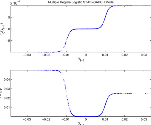
Example 1. Consider a three regime MLSTAR(1)-GARCH(1,1) model, where the transition variable is yt−1,

φ00=−0.001, φ10=0.001, φ20=0.001, φ01=−0.001, φ11=0.001, φ21=0.001, γ1=1000, γ2=1000, c1=−0.01,

c2=0.01, ω=10−5, α=0.05, and β=0.85. Fig. 1 shows the scatter plot f0(yt₋1) and f1(yt₋1) versus yt₋1. One

characteristicofsuchaspecificationisthatthelinearparametersineachlimitingregimesareallowedtobedifferent.

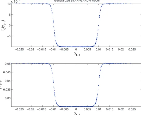
Example 2. Consider a three regime GSTAR(1)-GARCH(1,1) model, where the transition variable is yt−1,

φ00=−0.001, φ10=0.002, φ01=0.025, φ11=0.025, γ=100, 000, c1=−0.01, c2=0.01, ω=10−5, α=0.05, and β=0.85.Fig.2showsthe scatterplotf0(yt₋1)andf1(yt₋1) versusyt₋1.Asdistinct fromtheMLSTAR model,the

linearparametersineachlimitingextremeregimearerestrictedtobeequal.

Example 3. Consider a three regime ESTAR(1)-GARCH(1,1) model, where the transition variable is yt−1,

φ00=−0.001,φ10=0.002,φ01=0.025,φ11=0.025,γ=100,000,c=0,ω=10−5,α=0.05,andβ=0.85.Fig.3shows thescatterplotf0(yt₋1)andf1(yt₋1)versusyt₋1.Asinthepreviousexample,thelinearparametersineachlimiting

−0.03 −0.02 −0.01 0 0.01 0.02 0.03 −5 0 5 x 10−4 y t−1 f 0 (y t−1 )

Multiple Regime Logistic STAR−GARCH Model

−0.03 −0.02 −0.01 0 0.01 0.02 0.03 0.01 0.02 0.03 0.04 y t−1 f 1 (y t−1 )

Fig.1.Upperpanel:f0(yt−1)versusyt−1foronerealizationofthemodeldescribedinExample1.Lowerpanel:f1(yt−1)versusyt−1foronerealization

ofthemodeldescribedinExample1.

3. Probabilisticproperties

In thissection,onlyfirst-ordermodels willbeconsidered, whileinSection4 generalnonlinear modelswillbe analyzed.Considerthefollowingsetofassumptions.

Assumption 1 (ErrorTerm). The sequence{ηt} of IID(0,1) randomvariablesisdrawn fromacontinuous(with

respecttoLebesguemeasureontherealline),unimodal,positiveeverywheredensity,andboundedinaneighborhood of0.

Assumption2(ModelStructure). p=1andst=yt−1inEq.(1).

Assumption3(IdentifiabilityandPositivenessoftheVariance). Theparametersofthemodeldefinedby(1)–(3)satisfy thefollowingrestrictions:(R.1a)γi>0,i=1,...,m,andc1<c2<···<cmin(4);(R1.b)γ>0andc1≤c2≤···≤cm

in(6);(R.1c)γ>0in(8);and(R.2)ω>0,α>0,andβ>0.

Assumption1isstandard.Notethatwedonotassumesymmetryofthedistribution,whichisparticularlyuseful whenmodellingfinancialtimeseries.Assumption2forcesthemodeltobeoffirst-order.Thiswillbecrucialtothe resultsinthissection,butwillberelaxedinSection4.Therestrictions(R.1a)–(R.1c)inAssumption3areimportant toguaranteethatthemodelisgloballyidentifiable.Restriction(R.2)isasufficientconditionforht>0withprobability

one.

Notethatzt=(yt,ht,ηt)isaMarkovchainwithhomogenoustransitionprobability,expressedas

−0.025 −0.02 −0.015 −0.01 −0.005 0 0.005 0.01 0.015 0.02 0.025 −5 0 5 10x 10 −4 y t−1 f 0 (y t−1 )

Generalized STAR−GARCH Model

−0.025 −0.02 −0.015 −0.01 −0.005 0 0.005 0.01 0.015 0.02 0.025 0.03 0.035 0.04 0.045 0.05 y t−1 f 1 (y t−1 )

Fig.2.Upperpanel:f0(yt−1)versusyt−1foronerealizationofthemodeldescribedinExample2.Lowerpanel:f1(yt−1)versusyt−1foronerealization

ofthemodeldescribedinExample2.

where F(zt−1)= ⎡ ⎢ ⎢ ⎣

f0(yt−1)+f1(yt−1)yt−1 ω+β+αη2_t−1ht−1 0 ⎤ ⎥ ⎥ ⎦ andet=(εt,0,ηt).

Thefollowingtheoremsstatethenecessaryconditionsforstrictstationarityandgeometricergodicityofthe STAR-GARCHmodelsconsideredinthispaper.

Theorem1(Stationarity–MRLSTAR(1)-GARCH(1,1)model). Defineφ=_im₌₀φi1.UnderAssumptions1and2,

andif(R.1a)inAssumption3holds,theprocess{yt,t∈Z}definedbyEqs.(1)–(3)and(4)isstrictlystationaryand

geometricallyergodicifα+β<1,|φ01|<1and|φ|<1.Furthermore,theprocess{zt,t∈Z}admitsauniquecausal

expansion.

Theorem2(Stationarity–GSTAR(1)-GARCH(1,1)model). Setφ=φ01+φ11.UnderAssumption1,andif(R.1b)

inAssumption3holds,theprocess{yt,t∈Z}definedbyEqs.(1)–(3)and(6)isstrictlystationaryandgeometrically

ergodicifα+β<1,|φ01|<1and|φ|<1.Furthermore,theprocess{zt,t∈Z}admitsauniquecausalexpansion.

Theorem3(Stationarity–ESTAR(1)-GARCH(1,1)model). Setφ=φ01+φ11.UnderAssumption1,andif(R.1c)in Assumption3holds,theprocess{yt,t∈Z}definedbyequations(1)–(3)and(8)isstrictlystationaryandgeometrically

−0.03 −0.02 −0.01 0 0.01 0.02 2 4 6 8 10x 10 −4 y t−1 f 0 (y t−1 )

Exponential STAR−GARCH Model

−0.03 −0.02 −0.01 0 0.01 0.02 0.038 0.04 0.042 0.044 0.046 0.048 0.05 f 1 (y t−1 ) y t−1

Fig.3.Upperpanel:f0(yt−1)versusyt−1foronerealizationofthemodeldescribedinExample3.Lowerpanel:f1(yt−1)versusyt−1foronerealization

ofthemodeldescribedinExample3.

Iftheconditionsoftheabovetheoremsaremet,theprocesses{yt}and{ht}havethefollowingcausalexpansions:

yt=λ0,t−1+ ∞ j=1 j−1 k=0

f0(yt−1−j)f1(yt−1−k)+f1(yt−1−k)εt−j

, (11) ht =ω ⎡ ⎣1+ ∞ j=1 j k=1 β+αη2_t−i ⎤ ⎦. (12)

4. Parameterestimationandasymptotictheory

Inthissection,wediscusstheestimationofgeneralnonlinearautoregressivemodelswithGARCH(1,1)errors.The STAR-GARCHmodelsanalyzedpreviouslyarejustspecialcasesofthegeneralmodel.

Considerthefollowingassumption.

Assumption4. TheR-valuedprocess{yt,t∈Z}followsthefollowingnonlinearautoregressiveprocesswithGARCH

errors(NAR-GARCH): yt=g(yt−1;λ)+εt, (13) εt=ηt ht, (14) ht =ω+αε2t−1+βht−1, (15) whereyt−1= yt−1,...,yt−p andηt∼IID(0,1).

Assumption5. Thenonlinearfunctiong(yt−1;λ)satisfiesthefollowingsetofrestrictions: 1. g(yt−1;λ)iscontinuousinλandmeasurableinyt−1.

2. g(yt₋1;λ)isparameterizedsuchthattheparametersarewelldefined. 3. g(yt₋1;λ)andεtareindependent.

4. E|g(yt−1;λ)|q<∞,q=1,2,4. 5. Eexpgy_t−1;λq<∞,q=1,2,4. 6. E_∂∂_λg(yt−1;λ) q <∞,q=1,2,4. 7. E_∂λ∂_∂2_λg(yt−1;λ) q <∞,q=1,2.

Setψ=λ,π,whereλisthevectorofparametersoftheconditionalmean,asdefinedinSection2,andπ=(ω, α,β)isthevectorofparametersoftheconditionalvariance.Asthedistributionofηtisunknown,theparametervector ψisestimatedbythequasi-maximumlikelihood(QML)method.Considerthefollowingassumption.

Assumption6. Thetrueparametervector,ψ0∈Ψ ⊆RN,isintheinteriorofΨ,acompactandconvexparameter space,whereN=dim(λ)+dim(π)isthetotalnumberofparameters.

Thequasi-log-likelihoodfunctionoftheNAR-GARCHmodelisgivenby: LT(ψ)= 1 T T t=1 t(ψ)= 1 T T t=1 −1 2ln(2π)− 1 2ln(ht)− ε2_t 2ht . (16)

Notethat theprocesses yt andht,t≤0, are unobserved,andhenceare onlyarbitrary constants.Thus,LT(ψ)isa

quasi-log-likelihoodfunctionthatisnotconditionalonthetrue (y0,h0),makingitsuitableforpracticalapplications. However,toprovetheasymptoticpropertiesoftheQMLE,itismoreconvenienttoworkwiththeunobservedprocess

εu,t,hu,t

: t=0,±1,±2,....

Theunobservedquasi-log-likelihoodfunctionconditionalonF0=(y0,y−1,y−2,...)is Lu,T(ψ)= 1 T T t=1 u,t(ψ)= 1 T T t=1 −1 2ln(2π)− 1 2ln(hu,t)− ε2_u,t 2hu,t . (17)

ThemaindifferencebetweenLT(ψ)andLu,T(ψ)isthattheformerisconditionalonanyinitialvalues,whereasthe

latterisconditionalonaninfiniteseriesofpastobservations.Inpracticalsituations,theuseof(17)isnotpossible. Let ψT =argmaxψ∈ΨLT(ψ)=argmaxψ∈Ψ 1 T T t=1 t(ψ) , and

ψu,T =argmaxψ∈ΨLu,T(ψ)=argmaxψ∈Ψ

1 T T t=1 u,t(ψ) . DefineL(ψ)=Elu,t(ψ)

.Inthefollowingsubsection,wediscusstheexistenceofL(ψ)andtheidentifiabilityof theNAR-GARCHmodels.Then,inSection4.2,weprovetheconsistencyofψT andψu,T.Wefirstprovethestrong

consistencyofψu,T,andthenshowthat

sup

ψ∈Ψ

_{Lu,T(ψ)−LT(ψ)}a.s.

→0,

sothattheconsistencyofψT follows.AsymptoticnormalityofbothestimatorsisconsideredinSection4.3.Weprove

4.1. ExistenceoftheQMLE

ThefollowingtheoremprovestheexistenceofL(ψ).ItisbasedonTheorem2.12inWhite(1994),whichestablishes thatL(ψ)existsundercertainconditionsofcontinuityandmeasurabilityofthequasi-log-likelihoodfunction.

Theorem4. UnderAssumptions1and2,L(ψ)exists,isfinite,andisuniquelymaximizedatψ0.

4.2. Consistency

ThefollowingtheoremstatesthesufficientconditionsforstrongconsistencyoftheQMLE.

Theorem5. UnderAssumptions1–6,theQMLEofψisstronglyconsistentforψ0,ψa.s.→ψ0.

4.3. Asymptoticnormality

First,weintroducethefollowingmatrices:

A(ψ0)=E −

∂

2 lu,t(ψ)

∂

ψ

∂

ψ ψ0 , B(ψ0)=E

∂

u,t(ψ)

∂

ψ ψ0

∂

u,t(ψ)

∂

ψ ψ0 , and AT(ψ)= 1 T T t=1 1 2ht ε2_t ht − 1

∂

2ht

∂

ψ

∂

ψ − 1 2h2t 2ε 2 t ht − 1

∂

ht

∂

ψ

∂

ht

∂

ψ + εt h2t

∂

εt

∂

ψ

∂

ht

∂

ψ +

∂

ht

∂

ψ

∂

εt

∂

ψ + 1 ht

∂

εt

∂

ψ

∂

εt

∂

ψ +εt

∂

2εt

∂

ψ , (18) BT(ψ)= 1 T T t=1

∂

t(ψ)

∂

ψ

∂

t(ψ)

∂

ψ = 1 T T t=1 1 4h2t ε2_t ht − 1 2

∂

ht

∂

ψ

∂

ht

∂

ψ + ε2_t ht

∂

εt

∂

ψ

∂

εt

∂

ψ− εt 2h2t ε2_t ht − 1

∂

ht

∂

ψ

∂

εt

∂

ψ +

∂

εt

∂

ψ

∂

ht

∂

ψ . (19)

Considertheadditionalassumption:

Assumption7. Thereexistsnosetofcardinal2suchthatPr[ηt∈]=1.

AsinFrancqandZakoïan(2004),Assumption7isnecessaryforidentifyingreasonswhenthedistributionofηtis

non-symmetric.

Thefollowingtheoremstatestheasymptoticnormalityresult.

Theorem6. UnderAssumptions1–7andtheadditionalassumptionEε4_t=μ4<∞,then

T1/2(ψT−ψ0)

d

→N(0,Ω), (20)

whereΩ=A(ψ0)−1B(ψ0)A(ψ0)−1.IfthedistributionofηtissymmetricandE

η4_t=κ4,then A(ψ₀)= ⎛ ⎝A1 0 0 A2 ⎞ ⎠ , B(ψ₀)= ⎛ ⎝B1 0 0 B2 ⎞ ⎠,

Table1

Simulation:Estimationresults.

Parameter Truevalue 500observations

Model1 Model2 Model3

Mean Std.Dev. Mean Std.Dev. Mean Std.Dev.

φ00 −0.001 −0.0028 0.0190 −0.0026 0.0102 −0.0066 0.1005 φ10 0.002 0.0071 0.0387 0.0038 0.0108 0.0077 0.1005 φ20 0.001 0.0004 0.0421 – – – – φ01 0.025 0.0350 0.198 0.0142 0.1323 0.0599 0.5974 φ11 0.25 0.1342 0.3390 0.4171 0.1326 0.3872 0.5978 φ21 0.001 0.0002 0.0531 – – – –

γ1 1000 1000 1.91e−7 1000 1.71e−8 1000 1.69e−8

γ2 1000 1000 2.01e−7 – – – –

c1 −0.01 −0.0093 0.0115 −0.0101 0.0105 −0.0107 0.0127

c2 0.01 0.0101 0.0099 – – – –

ω 10e−5 16.78e−5 6.01e−4 17.43e−5 4.01e−4 17.83e−5 3.56e−4

α 0.05 0.0650 0.0600 0.0686 0.0578 0.0685 0.0577

β 0.85 0.6315 0.3347 0.6264 0.3399 0.6389 0.3400

Parameter Truevalue 1000observations

Model1 Model2 Model3

Mean Std.Dev. Mean Std.Dev. Mean Std.Dev.

φ00 −0.001 −0.0024 0.0091 −0.00212 0.0076 −0.0034 0.0144 φ10 0.002 0.0015 0.0232 0.0032 0.0078 0.0045 0.0145 φ20 0.001 0.0006 0.0236 – – – – φ01 0.025 0.0204 0.0825 0.0465 0.8080 0.0371 0.6172 φ11 0.25 0.171 0.273 0.3615 0.809 0.3261 0.6538 φ21 0.001 0.0005 0.0181 – – – –

γ1 1000 1000 2.88e−9 1000 2.58e−8 1000 2.27e−8

γ2 1000 1000 1.59e−8 – – – –

c1 −0.01 −0.0096 0.0004 −0.0106 7.67e−5 −0.0106 5.0e−5

c2 0.01 0.0092 0.0001 0.0093 4.35e−5 – –

ω 10e−5 15.09e−5 6.01e−5 16.46e−5 6.40e−5 16.51e−5 6.75e−5

α 0.05 0.0673 0.0368 0.0708 0.357 0.0707 0.0351

β 0.85 0.772 0.3223 0.7483 0.3143 0.7621 0.3063

Parameter Truevalue 5000observations

Model1 Model2 Model3

Mean Std.Dev. Mean Std.Dev. Mean Std.Dev.

φ00 −0.001 −0.0006 0.0022 −0.0015 0.00194 −0.0017 0.0026 φ10 0.002 0.0028 0.0598 0.0024 0.00206 0.0023 0.0026 φ20 0.001 0.0011 0.0089 – – – – φ01 0.025 0.0338 0.0554 0.0211 0.0173 0.0235 0.2601 φ11 0.25 0.2232 0.1399 0.2663 0.1732 0.2854 0.2602 φ21 0.001 0.0009 0.0452 – – – –

γ1 1000 1000 1.30e−9 1000 5.60e−9 1000 1.907e−8

γ2 1000 1000 8.23e−10 – – – –

c1 −0.01 −0.0098 4.06e−5 −0.0104 2.92e−5 −0.0102 1.25e−5

c2 0.01 0.0126 0.0001 0.0098 7.80e−6 – –

ω 1e−5 15.85e−5 5.66e−5 15.67e−5 5.90e−5 15.55e−5 5.84e−5

α 0.05 0.0598 0.0107 0.0596 0.0106 0.0594 0.0106

β 0.85 0.781 0.0616 0.7831 0.0642 0.7846 0.0638 Thetableshowsthemeanandthestandarddeviationofquasi-maximumlikelihoodestimatoroftheparametersofModels1–3over1000replications. Wereporttheresultswithboth1000and5000observations.

with A1=E 1 h2t

∂

ht

∂

λ

∂

ht

∂

λψ0 +E 2 h2t

∂

εt

∂

λ

∂

εt

∂

λψ0 , A2=E 1 h2_t

∂

ht

∂

π

∂

ht

∂

π ψ0 , B1=(κ4−1)E 1 h2t

∂

ht

∂

λ

∂

ht

∂

λ ψ0 +4E 1 h2t

∂

εt

∂

λ

∂

εt

∂

λψ0 , and B2=(κ4−1)E 1 h2_t

∂

ht

∂

π

∂

ht

∂

πψ0 .

Furthermore,thematricesA(ψ0)andB(ψ0)areconsistentlyestimatedbyAT(ψ)andBT(ψ),respectively.

Notethatweallowtheerrortermηttobenon-Gaussian.However,werequitethat

t=

√

htηttohavefinite

fourth-ordermomentinordertoachieveasymptoticnormalityoftheestimates.Inthecaseofveryfattailederrors,possibly withouttheexistenceofhigher-ordermoments,thecurrentresultsinthispaperwillnotbevalidanymore.

5. MonteCarlosimulations

Inthissectionwereporttheresultsofasimulationstudydesignedtoevaluatethefinitesamplepropertiesofthe QMLE.Weconsiderthreedifferentmodelspecificationsasdescribedbelow:

• Model1:MLSTAR(1)-GARCH(1,1)Athree regime model wherethe transition variable is yt−1,φ00=−0.001, φ10=0.002,φ20=0.001,φ01=0.025,φ11=0.25,φ21=0.001,γ1=1000,γ2=1000,c1=−0.01,c2=0.01,ω=10−5, α=0.05,andβ=0.85.

• Model2:GSTAR(1)-GARCH(1,1) A three regime model where the transition variable is yt−1, φ00=−0.001, φ10=0.002,φ01=0.025,φ11=0.25,γ1=1000,c1=−0.01,c2=0.01,ω=10−5,α=0.05,andβ=0.85.

• Model3:ESTAR(1)-GARCH(1,1)Consideratworegimemodelwherethetransitionvariableisyt−1,φ00=−0.001,

φ10=0.002,φ01=0.025,φ11=0.25,γ1=1000,c1=−0.01,ω=10−5,α=0.05,andβ=0.85.

The resultsare illustrated inTable1.The tableshows the averageandthe standarddeviation of the estimates over1000replications.Aswecanseefromthetable,theestimatesareratherpreciseandimproveasthesamplesize increases.

6. Concludingremarks

Inthispaperwehavederivedsufficientconditionsforstrictstationarityandgeometricergodicityofthreedifferent classesoffirst-orderSTAR-GARCHmodels.Thisisimportantinordertofindtheconditionsunderwhichthetraditional LMlinearitytestsarevalid.TheasymptoticpropertiesoftheQMLEhavealsobeenconsidered.Wehaveprovedthat theQMLEisconsistentandasymptoticallynormalunderweakconditions.Thesenewresultsshouldbeimportantfor theestimationofSTAR-GARCHmodelsinfinancialeconometrics.

AppendixA. ProofsofTheorems1–3

TheproofsofthetheoremsarebasedonChanetal.(1985),andmakesuseoftheresultsinTweedie(1988). LetAbeak×kmatrixthenρ(A)denotesthespectralradiusofA.Thatis,themaximumabsoluteeigenvalueofA. LetAbeaboundedsetofmatricesandAk =#k_i=1Ai:Ai∈A,i=1,...,k

$

,thenρ_∗(A)denotesthejointspectral radiusofthesetA,thatis

ρ_∗(A)=limsup k→∞ sup A_∈Ak ||A|| 1/ k

Forthepurposeofthefollowingproofs,considerafirst-orderSTAR-GARCHmodelsdefinedas:

yt =f0(yt−1)+f1(yt−1)yt−1+εt, (A.1)

εt =ηt ht, (A.2) and ht=ω+αε2t−1+βht−1, (A.3) where f0(yt−1) =φ00+φ10G(yt−1;γ,c) f1(yt−1) =φ01+φ11G(yt−1;γ,c)

andG(yt−1;γ,c)isatwicedifferentiablefunctionwiththerangeequalsto[0,1].Now,letzt =(yt,yt−1,ht)thenthe

STAR(1)-GARCH(1,1)modelcouldhavethefollowingMarkovianrepresentation

zt =F(zt−1,ηt) (A.4) where F(zt−1,ηt)= ⎡ ⎢ ⎢ ⎣

f0(yt−1)+f1(yt−1)yt−1 yt−1 h(zt−1) ⎤ ⎥ ⎥ ⎦+ ⎡ ⎢ ⎣ h(zt−1)1/2ηt 0 0 ⎤ ⎥ ⎦. (A.5)

TheproofofergodicityforSTAR(1)-GARCH(1,1)isbasedontheresultsfromMeitzandSaikkonen(2008),which providedsufficientconditionstoverifyergodicityforthefollowingprocess:

yt =f(yt−1,...,yt−p)+h1t/2ηt

ht =g(ut−1,ht−1)

ut =yt−f(yt−1,...,yt−p)

(A.6)

wherefisanonlinearfunctionsuchthatf(yt−1,...,yt−p)definedanonlinearautoregressiveprocessoforderp.htis

apositivefunctionofyssuchthats<tandηtisasequenceofiid(0,1)randomvariablesindependentof{ys:s<t}.

Model(A.6)canberewrittenasaMarkovchainsuchthat

whereZt=(yt,yt−1,...,yt−p,ht)and F(Zt−1,ηt)= ⎛ ⎜ ⎜ ⎜ ⎜ ⎜ ⎜ ⎜ ⎝ f(yt−1,...,yt−p) yt−1 .. . yt−p ht(Zt−1) ⎞ ⎟ ⎟ ⎟ ⎟ ⎟ ⎟ ⎟ ⎠ + ⎛ ⎜ ⎜ ⎜ ⎜ ⎜ ⎜ ⎜ ⎝ ht(Zt−1)1/2ηt 0 .. . 0 0 ⎞ ⎟ ⎟ ⎟ ⎟ ⎟ ⎟ ⎟ ⎠

MeitzandSaikkonen(2008)showedthatthefollowingconditionsaresufficienttoensuregeometricergodicityfor theMarkovchain,Zt.

Condition1. ηt hasa(Lebesgue)densitywhichispositiveandlowersemicontinuousonR.Furthermore,forsome

realr≥1,E(η2tr)<∞.

Condition2. Thefunctionfisoftheform

f(x)=a(x)x+b(x), x∈Rp;

wherethefunctionsa:Rp→Rpandb:Rp→Raresmoothandbounded.

Condition3. Given a(x) from the previous assumption, rewrite a(x)=(a1(x), a2(x), ..., ap(x)) and define the

(p+1)×(p+1)matrixsuchthat

A(x)= ⎛ ⎜ ⎜ ⎜ ⎜ ⎝ a1(x) a2(x) ... ap(x) 0 1 0 ... 0 0 .. . ... . .. ... ... 0 0 ... 1 0 ⎞ ⎟ ⎟ ⎟ ⎟ ⎠.

Thenthereexistsamatrixnorm||•||inducedbyavectornormsuch that||A||≤ρ

∀

A∈Awhere A={A(x):x∈Rp}andsome0<ρ<1.

Condition4. a. Thefunctiong:R×R₊→R₊issmoothandforsomeg>0, inf

(u,x)∈R×R₊g(u,x)=g. b. Forallx∈R₊,g(u,x)→∞asu→∞.

c.

∃

h∗∈R₊suchthatthesequencehk(k=1,2,...)definedbyhk=g(0,hk−1),k=1,2,...convergesto h*ask→∞forallh0∈R+.Ifg(u,x)≥h*forallu∈Randallx≥h*itsufficesthatthisconvergence holdsforallh0≥h*.

d. Thereexistnonnegativerealnumbersaandc,andaBorelmeasurablefunctionψ:R→R₊such that

g(x1/2ηt,x)≤(a+ψ(ηt))x+c

∀

x∈R₊. Furthermore, a+ψ(0)<1 and E[(a+ψ(ηt))r]<1 where the real number r≥1 is as in

Assumption1.

e. Foreachinitialvaluez0∈Z,thereexitsacontrolsequencee(0)₁ ,...,e(0)_p+2suchthatthe(p+2)×(p+2) matrix

∇

F_p(0)₊₂=

∂

∂

e1Fp+2(z0,e (0) 1 ,...,e (0) p+2):...:

∂

∂

ep+2 Fp+2(z0,e(0)1 ,...,e (0) p+2) isnon-singular.

A.1. ProofofTheorem1

ItissufficienttoverifyConditions1to5inMeitzandSaikkonen(2008).Condition1issatisfiedbyAssumption (1)withr=1.Definef(yt−1)=λ0,t−1+λ1,t−1yt−1andlet

a(x) =θ0+θ1G(x;γ,c) b(x) =φ0+φ1G(x;γ,c) g(u,x) =ω+αu2+βx

Hence,f(x)=a(x)x+b(x) andhenceCondition2 issatisfied.Following Liebscher(2005),asufficient conditionto ensureCondition3is ρ_∗({1,2})<1 where 1= φ0 0 1 0 , 2= φ0+φ1 0 1 0

Letbij denotesthe(i,j)elementofthematrixBfori,j=1,2 suchthatB=

k

i=1Ai,whereAi∈{1,2}

∀

i=1,

...,k.Giventhestructureof1and2,itiseasytoverifythatb12=0andb22=0forallk∈Z+.Thisimpliesthe eigenvaluesofBare0andφl₀(φ0+φ1)mforsomel,m∈Z+.Giventheassumptionsthat|φ0|<1,|φ0+φ1|<1and |φ0(φ0+φ1)|<1,itisobviousthatφl₀(φ0+φ1)m→0ask→∞.Hence,Condition3issatisfied.

Letg=ω,giventhatω>0,α≥0andβ≥0then inf

u,x∈R×R₊g(u,x)=ω=g.

Inaddition,

∀

x∈R₊,g(u,x)→∞asu→∞.Sinceα+β<1,α>0andβ>0therefore0<β<1.Now, hk=g(0, hk−1)=ω+βhk−1andforanynonnegativeinitialvalueh0<∞,itisstraightforwardtoshowthat

hk=

ω(1−βk−1) 1−β +β

k_h0.

Hence, hk→ ₁₋ω_β as k→∞. Moreover,let c=ω, a=β andψ(ηt)=αη2t then g(x1/2ηt, x)=(a+ψ(ηt))x+c,with a+ψ(0)=β<1.FromCondition1,r=1andthereforeE(a+ψ(ηt))r=E(a+ψ(ηt))=α+β<1.HenceCondition

4issatisfied.

ToverifyCondition5,itisusefultonotethatp=1sothat

∇

F_p(0)₊₁=

∇

F₃(0)suchthat

∇

F₃(0)= ⎛ ⎜ ⎜ ⎜ ⎜ ⎜ ⎜ ⎜ ⎝

∂

y3

∂

e1

∂

y3

∂

e2 h1₃/2

∂

y2

∂

e1 h1₂/2 0

∂

h3

∂

e1

∂

h3

∂

e2 0 ⎞ ⎟ ⎟ ⎟ ⎟ ⎟ ⎟ ⎟ ⎠ Letthe controlsequencebe

e(0)₁ ,e(0)₂ ,e(0)₃

=(e1,0,0) where|e1|<∞.Notethat h_i1/2>0 fori=2,3.Evaluating

∇

F₃(0)atthespecifiedcontrolsequencegives

∂

h3

∂

e1 =β

∂

h2

∂

e1 >0

∂

h3

∂

e2 =2αe2h2=0

andhence,thereexistsacontrolsequencesuchthat

∇

F₃(0)isnon-singularandthereforeConditions1to5aresatisfied. Thiscompletestheproof.

A.2. ProofofTheorem3

TheproofofTheorem3followsthesamelinesastheoneofTheorem1.

A.3. ProofofTheorem2

TheproofofTheorem2followsthesamelinesastheoneofTheorem1.

AppendixB. ProofsofTheorems4–6

B.1. ProofofTheorem4

ItiseasytoseethatF(zt),asin(10),isacontinuousfunctionintheparametervectorψ.Similarly,wecanseethat F(zt)iscontinuousinzt,andthereforeismeasurable,foreachfixedvalueofψ.

Furthermore,undertherestrictionsinAssumption2,andifthestationarityconditionsofeitherTheorem1,2,or 3aresatisfied,thenE

sup ψ∈Ψ h_u,t<∞andE sup ψ∈Ψ

y_u,t<∞.ByJensen’sinequality,E sup ψ∈Ψ lnhu,t <∞. Thus,Elu,t(ψ)<∞

∀

ψ∈Ψ.

Leth0,tbethetrueconditionalvarianceandε0,t=h01/,t2ηt.InordertoshowthatL(ψ)isuniquelymaximizedatψ0,

rewritethemaximizationproblemas

max ψ∈Ψ L(ψ)−L(ψ0) =max ψ∈Ψ ' E ln h0,t hu,t − ε2t hu,t + 1 ( . (B.1)

Writingεt=εt−ε0,t+ε0,t,Eq.(B.1)becomes

max ψ∈Ψ L(ψ)−L(ψ0) =max ψ∈Ψ ) E ln h0,t hu,t −h0,t hu,t +1 −E [εt−ε0,t]2 hu,t −E 2ηth10/,t2(εt−ε0,t) hu,t * =max ψ∈Ψ ) E ln h0,t hu,t −h0,t hu,t + 1 −E [εt−ε0,t]2 hu,t * , (B.2) where E 2ηth10/,t2(εt−ε0,t) hu,t =0 bytheLawofIteratedExpectations.

Notethat,foranyx>0,m(x)=ln(x)−x≤0,sothat

E ln h0,t hu,t −h0,t hu,t ≤0.

Furthermore,m(x)ismaximizedatx=1.Ifx =/ 1,m(x)<m(1),implyingthatE[m(x)]≤E[m(1)],withequalityonly ifx=1a.s..However,thiswilloccuronlyif h0,t

hu,t =1,a.s..Inaddition, E [εt−ε0,t]2 hu,t =0

ifandonlyifεt=ε0,t.Hence,ψ=ψ0.Thiscompletestheproof. B.2. ProofofTheorem5

FollowingWhite(1994),Theorem3.5,ψ_u,Ta.s.→ψ0ifthefollowingconditionshold: (1) TheparameterspaceΨ iscompact.

(2) Lu,T(ψ)iscontinuousinψ∈Ψ.Furthermore,Lu,T(ψ)isameasurablefunctionofyt,t=1,...,T,forallψ∈Ψ.

(3) L(ψ)hasauniquemaximumatψ0. (4) lim

T→∞_ψsup_∈Ψ

_Lu,T(ψ)−L(ψ)=0,a.s..

Condition(1) holds by assumption.Theorem 4 shows that Conditions(2) and(3) are satisfied.By Lemma 1, Condition(4)isalsosatisfied.Thus,ψu,T

a.s.

→ψ0. Lemma2showsthat

lim

T→∞_ψsup_∈Ψ

_Lu,T(ψ)−LT(ψ)=0a.s.,

implyingthatψT a.s.

→ψ0.Thiscompletestheproof.

B.3. ProofofTheorem6

WestartbyprovingasymptoticnormalityoftheQMLEusingtheunobservedlog-likelihood.Whenthisisshown, theproofusingtheobservedlog-likelihoodisimmediatebyLemmas2and4.AccordingtoTheorem6.4inWhite (1994),toprovetheasymptoticnormalityoftheQMLEweneedthefollowingconditionsinadditiontothosestated intheproofofTheorem5:

(5) Thetrueparametervectorψ0isinteriortoΨ. (6) Thematrix AT(ψ)= 1 T T t=1

∂

2lt(ψ)

∂

ψ

∂

ψ

existsa.s.andiscontinuousinΨ. (7) ThematrixAT(ψ)

a.s.

→A(ψ0),foranysequenceψT,suchthatψT a.s.

→ψ0. (8) Thescorevectorsatisfies

1 √ T T t=1

∂

lt(ψ)

∂

ψ d →N(0,B(ψ0)).

Condition(5)issatisfiedbyassumption.Condition(6)followsfromthefactthatlt(ψ)isdifferentiableofordertwo

Lemma4.Furthermore,Lemmas3and5impliesthatCondition(7)issatisfied.InLemma6,weprovethatcondition (8)isalsosatisfied.Thiscompletestheproof.

AppendixC. Lemmas

Lemma1. SupposethatytfollowsaSTAR-GARCHmodelsatisfyingtherestrictionsinAssumptions1and2,andthe stationarityandergodicityconditionsaremet.Then,

lim

T→∞_ψsup_∈Ψ

_{Lu,T(ψ)−L(ψ)=0,}a.s..

Proof. Setg(Yt,ψ)=lu,t(ψ)−E

lu,t(ψ) ,whereYt = yt,yt−1,yt−2,... .Hence,Eg(Yt,ψ) =0.Itisclear that E sup ψ∈Ψ|g(Yt,ψ)|

<∞ by Theorem 4. Furthermore, as g(Yt, ψ) is strictly stationary and ergodic, then

lim

T→∞_ψsup_∈Ψ

T−1T_t=1g(Yt,ψ)=0,a.s..Thiscompletestheproof.

Lemma2. UndertheassumptionsofLemma1,

lim

T→∞_ψsup_∈Ψ

_{Lu,T(ψ)−LT(ψ)=0,}a.s..

Proof. First,write ht = t−1 i=0 βi ω+αε2_t−1−i +βth0 and hu,t =βt−1 ω+αε2_u,0 + t−2 i=0 βi ω+αε2_t−1−i +βthu,0, suchthat ht−hu,t =βt−1α ε2₀−ε2_u,0+βth0−hu,0 ≤βt−1αε2₀−ε2_u,0+βth0−hu,0.

Underthestationarityoftheprocess,andif(R.2)inAssumption2andthelog-momentconditionhold,itisclearthat 0<β<1.Furthermore,hu,0andε20,uarewelldefined,as

Pr sup ψ∈Ψ hu,0>K1 →0asK1→∞,andPr sup ψ∈Ψ ε2_u,0>K2 →0asK2→∞. Thus, sup ψ∈Ψ ht−hu,t≤Khρt1, a.s., and sup ψ∈Ψ ε2₀−ε2_u,0≤Kερt2, a.s.,

whereKhandKεarepositiveandfiniteconstants,0<ρ1<1,and0<ρ2<1.Hence,asht>ωandlog(x)≤x−1, sup ψ∈Ψ l_t−lu,t ≤ sup ψ∈Ψ ε2_t hu,t−ht hthu,t +log 1+ht−hu,t hu,t ≤ sup ψ∈Ψ 1 ω2 Khρt1ε2t +sup ψ∈Ψ 1 ω Khρt1, ,a.s..

FollowingthesameargumentsasintheproofofTheorems2.1and3.1inFrancqandZakoïan(2004),itcanbeshown that

lim

T→∞_ψsup_∈Ψ

_Lu,T(ψ)−LT(ψ)=0, a.s..

Thiscompletestheproof.

Lemma3. UndertheconditionsofTheorem6,

E

∂

lt(ψ)

∂

ψ ψ0 <∞, (C.1) E

∂

lt(ψ)

∂

ψ ψ0

∂

lt(ψ)

∂

ψ ψ0 <∞, (C.2) and E

∂

2lt(ψ)

∂

ψ

∂

ψ ψ0 <∞. (C.3) Proof. Set

∇

0lu,t ≡

∂

lu,t(ψ)

∂

ψ ψ0 ,

∇

0hu,t≡

∂

hu,t

∂

ψ ψ0 ,

∇

0εt≡

∂

εt

∂

ψψ0

∇

2 0lu,t ≡

∂

2lu,t(ψ)

∂

ψ

∂

ψ ψ0 ,

∇

2 0hu,t ≡

∂

2hu,t

∂

ψ

∂

ψψ0 , and

∇

2 0εt≡

∂

2εt

∂

ψ

∂

ψ ψ0 . Then,

∇

0lu,t = 1 2hu,t ε2_t hu,t − 1

∇

0hu,t− εt hu,t

∇

0 εt and

∇

2 0lu,t = ε2_t hu,t −1 1 2hu,t

∇

2 0hu,t− 1 2h2u,t 2 ε 2 t hu,t −1

∇

0hu,t

∇

0hu,t + εt h2u,t

∇

0εt

∇

0hu,t+

∇

0hu,t

∇

0εt + 1 hu,t

∇

0εt

∇

0εt+εt

∇

20εt .

Setψ=λ,π,where, as statedbefore, λ isthe vector of parametersof the conditional mean andπ is the vectorofparametersoftheconditionalvariance.AsintheproofofTheorem3.2inFrancqandZakoïan(2004),the derivativeswithrespect toπ are clearlybounded. Weproceed by analyzingthe derivatives withrespect toλ.As εt=yt−f0(yt−1;λ)−f1(yt−1;λ)yt−1,wehave

∂

εt

∂

λ =−

∂

f0(yt−1;λ)

∂

λ −

∂

f1(yt−1;λ)

∂

λ yt−1, (C.4)

∂

2εt

∂

λ

∂

λ =−

∂

2f0(yt−1;λ)

∂

λ

∂

λ −

∂

2f1(yt−1;λ)

∂

λ

∂

λ yt−1, (C.5)

∂

hu,t

∂

λ =2α ∞ i=0 βiεt−1−i

∂

εt−1−i

∂

λ , (C.6) and

∂

2hu,t

∂

λ

∂

λ =2α ∞ i=0 βi εt−1−i

∂

2εt−1−i

∂

λ

∂

λ +

∂

εt−1−i

∂

λ

∂

εt−1−i

∂

λ . (C.7)

Asthederivativesofthetransitionfunctionarebounded,ifthestrictstationarityandergodicityconditionshold, (C.4)–(C.7)areclearlybounded.Hence,theremainderoftheprooffollowsfromtheproofofTheorem3.2(part(i))in FrancqandZakoïan(2004).Thiscompletestheproof.

Lemma4. UndertheconditionsofTheorem6,A(ψ0)andB(ψ0)are nonsingularand,whenηthasasymmetric distribution,areblock-diagonal.

Proof. First,notethat(R1a)–(R1c)inAssumption2andAssumption7guaranteetheminimality(identifiability)of thedifferentspecificationsoftheSTARmodelsconsideredinthispaper.Therefore,theresultsfollowfromtheproof ofTheorem3.2(part(ii))inFrancqandZakoïan(2004).Thiscompletestheproof.

Lemma5. UndertheconditionsofTheorem6,

(a) lim T→∞_ψsup_∈Ψ ++ ++ + 1 T T t=1

∂

lu,t(ψ)

∂

ψ −

∂

lt(ψ)

∂

ψ ++ ++ +=0, a.s., (b) lim T→∞_ψsup_∈Ψ ++ ++ + 1 T T t=1

∂

2lu,t(ψ)

∂

ψ

∂

ψ −

∂

2lt(ψ)

∂

ψ

∂

ψ ++ ++ +=0, a.s, and (c) lim T→∞_ψsup_∈Ψ ++ ++ + 1 T T t=1

∂

2lu,t(ψ)

∂

ψ

∂

ψ −E

∂

2lu,t(ψ)

∂

ψ

∂

ψ ++ ++ +=0, a.s..

Proof. First,assumethath0andhu,0arefixedconstants.Itiseasytoshowthat

∂

ht

∂

λ −

∂

hu,t

∂

λ =2αβt−1ε0

∂

ε0

∂

λ −εu,0

∂

εu,0

∂

λ ≤2αβt−1_ε0

∂

ε0

∂

λ +εu,0

∂

εu,0

∂

λ <∞,

as0<β<1andytisstationaryandergodic.Hence,followingthesameargumentsasintheproofofTheorem3.2(part

(iii))inFrancqandZakoïan(2004),itisstraightforwardtoshowthat

lim T→∞_ψsup_∈Ψ ++ ++ + 1 T T t=1

∂

lu,t(ψ)

∂

λ −

∂

lt(ψ)

∂

λ ++ ++ +=0. Furthermore,as

∂

ht

∂

ω −

∂

hu,t

∂

ω =0

∂

ht

∂

α −

∂

hu,t

∂

α =ε 2 0−ε 2 u,0

∂

ht

∂

β −

∂

hu,t

∂

β =(t−1)β t−2_ε2 0−ε 2 u,0 +tβt−1(h0−hu,0),

Itisclearthat lim T→∞_ψsup_∈Ψ ++ ++ + 1 T T t=1

∂

lu,t(ψ)

∂

π −

∂

lt(ψ)

∂

π ++ ++ +=0.

Theproofofpart(a)isnowcomplete.Theproofofpart(b)followsalongsimilarlines.Theproofofpart(c)follows thesameargumentsasintheproofofTheorem3.2(part(v))inFrancqandZakoïan(2004).Thiscompletestheproof.

Lemma6. UndertheconditionsofTheorem6,

1 √ T T t=1

∂

lt(ψ)

∂

ψ ψ0 d →N(0,B(ψ0)). Proof. LetST = T

t=1c

∇

0lu,t,wherecisaconstantvector.ThenSTisamartingalewithrespecttoFt,thefiltration

generatedbyallpastobservationsofyt.Bythegivenassumptions,E[ST]>0.UsingthecentrallimittheoremofStout

(1974),

T−1/2ST d

→N(0,cB(ψ0)c). BytheCramér-Wolddevice,

T−1/2 T t=1

∂

lu,t(ψ)

∂

ψ ψ0 d →N0,B(ψ₀). ByLemma5, T−1/2 T t=1 ++ ++

∂

lu,t(ψ)

∂

ψ ψ0 −

∂

lt(ψ)

∂

ψ ψ0 ++ ++a.s. →0. Thus, T−1/2 T t=1

∂

lt(ψ)

∂

ψ ψ0 d →N(0,B0). Thiscompletestheproof.

References

An,H.,Chen,S.,1997.Anoteontheergodicityofnon-linearautoregressivemodel.Stat.Probabil.Lett.34,365–372. An,H.,Huang,F.,1996.Thegeometricalergodicityofnonlinearautoregressivemodels.Stat.Sinica6,943–956. Bacon,D.W.,Watts,D.G.,1971.Estimatingthetransitionbetweentwointersectinglines.Biometrika58,525–534. Berkes,I.,Horváth,L.,Kokoszka,P.,2003.GARCHprocesses:structureandestimation.Bernoulli9,201–227.

Bhattacharya,R.,Lee,C.,1995.Onthegeometricergodicityofnonlinearautoregressivemodels.Stat.Probabil.Lett.22,311–315. Bollerslev,T.,1986.Generalizedautoregressiveconditionalheteroskedasticity.J.Economet.21,307–328.

Bougerol,P.,Picard,N.M.,1992.StationarityofGARCHprocessesandofsomenon-negativetimeseries.J.Economet.52,115–127.

Boussama,F.,2000.NormalitéAsymptotiquedeL’EstimateurduPseudo-MaximumdeVraisemblancedúnModèleGARCH.C.R.Acad.Sci.Ser. I331,81–84.

Chan,F.,McAleer,M.,2002.MaximumlikelihoodestimationofSTARandSTAR-GARCHmodels:aMonteCarloAnalysis.J.Appl.Econom.17, 509–534.

Chan,K.S.,Petruccelli,J.D.,Tong,H.,Woolford,S.W.,1985.Amultiple-thresholdAR(1)model.J.Appl.Probabil.22(2),267–279. Chan,K.S.,Tong,H.,1986.Onestimatingthresholdsinautoregressivemodels.J.TimeSeriesAnal.7,179–190.

Chen,G.,Chen,M.,2001.OnaclassofnonlinearAR(p)modelswithnonlinearARCHerrors.Aust.N.Z.J.Stat.43,445–454. Chen,R.,Tsay,R.S.,1991.OntheergodicityofTAR(1)processes.Ann.Appl.Probab.1,613–634.

Chen,R.,Tsay,R.S.,1993.Functionalcoefficientautoregressivemodels.J.Am.Stat.Assoc.88,298–308.

Cline,D.,Pu,H.,1998.Verifyingirreducibilityandcontinuityofanonlineartimeseries.Stat.Probabil.Lett.40,139–148. Cline,D.,Pu,H.,1999.Geometricergodicityofnonlineartimeseries.Stat.Sinica9,1103–1118.

Cline,D.,Pu,H.,2004.StabilityandtheLyapounovexponentofthresholdAR-ARCHmodels.Ann.Appl.Probab.14,1920–1949. Comte,F.,Lieberman,O.,2003.AsymptotictheoryformultivariateGARCHprocesses.J.Multivar.Anal.84,61–84.

Engle,R.,Kroner,K.,1995.MultivariatesimultaneousgeneralizedARCH.Economet.Theory11,122–150.

Engle,R.F.,1982.AutoregressiveconditionalheteroskedasticitywithestimatesofthevarianceofUKinflations.Econometrica50,987–1007. Ferrante,M.,Fonseca,G.,Vidoni,P.,2003.Geometricergodicity,regularityoftheinvariantdistributionandinferenceforathresholdbilinear

Markovprocess.Stat.Sinica13,367–384.

Francq,C.,Zakoïan,J.-M.,2004.MaximumlikelihoodestimationofpureGARCHandARMA-GARCHprocesses.Bernoulli10,605–637. Goldfeld,S.M.,Quandt,R.,1972.NonlinearMethodsinEconometrics.NorthHolland,Amsterdam.

He,C.,Teräsvirta,T.,1999a.FourthmomentstructureoftheGARCH(p,q)process.Economet.Theory15,824–846. He,C.,Teräsvirta,T.,1999b.PropertiesofmomentsofafamilyofGARCHprocesses.J.Economet.92,173–192. Hwang,S.,Woo,M.-J.,2001.ThresholdARCH(1)processes:asymptoticinference.Stat.Probabil.Lett.53,11–20. Jeantheau,T.,1998.StrongconsistencyofestimatorsformultivariateARCHmodels.Economet.Theory14,70–86. Lee,C.,1998.Asymptoticsofaclassofpth-ordernonlinearautoregressiveprocesses.Stat.Probabil.Lett.40,171–177.

Lee,S.-W.,Hansen,B.E.,1994.AsymptotictheoryfortheGARCH(1,1)quasi-maximumlikelihoodestimator.Economet.Theory10,29–52. Li,W.K.,Lam,K.,1995.Modellingasymmetryinstockreturnsbyathresholdautoregressiveconditionalheteroscedasticmodel.TheStatistician

44,333–341.

Liebscher,E.,2005.Towardsaunifiedapproachforprovinggeometricergodicityandmixingpropertiesofnonlinearautoregressiveprocesses.J. TimeSeriesAnal.26,669–689.

Ling,S.,1999.OntheprobabilisticpropertiesofadoublethresholdARMAconditionalheteroscedasticitymodel.J.Appl.Probabil.36,1–18. Ling,S.,McAleer,M.,2002a.NecessaryandsufficientmomentconditionsfortheGARCH(r,s)andasymmetricpowerGARCH(r,s)models.

Economet.Theory18,722–729.

Ling,S.,McAleer,M.,2002b.StationarityandtheexistenceofmomentsofafamilyofGARCHprocesses.J.Economet.106,109–117. Ling,S.,McAleer,M.,2003.AsymptotictheoryforavectorARMA-GARCHmodel.Economet.Theory19,280–310.

Liu,J.,Li,W.K.,Li,C.W.,1997.Onathresholdautoregressionwithconditionalheteroscedasticvariances.J.Stat.Plan.Inference62,279–300. Lu,Z.,1998.Onthegeometricergodicityofanon-linearautoregressivemodelwithanautoregressiveconditionalheteroscedasticterm.Stat.Sinica

8,1205–1230.

Lu,Z.,Jang,Z.,2001.L1geometricergodicityofamultivariatenonlinearARmodelwithanARCHterm.Stat.Probabil.Lett.51,121–130. Lumsdaine,R.,1996.Consistencyandasymptoticnormalityofthequasi-maximumlikelihoodestimatorinIGARCH(1,1)andcovariancestationary

GARCH(1,1)models.Econometrica64,575–596.

Luukkonen,R.,Saikkonen,P.,Teräsvirta,T.,1988.Testinglinearityagainstsmoothtransitionautoregressivemodels.Biometrika75,491–499. Masry,E.,Tjostheim,D.,1995.NonparametricestimationandidentificationofnonlinearARCHtimeseries.Economet.Theory11,258–289. McAleer,M.,2005.Automatedinferenceandlearninginmodelingfinancialvolatility.Economet.Theory21,232–261.

McAleer,M.,Chan,F.,Marinova,D.,2007.Aneconometricanalysisofasymmetricvolatility:theoryandapplicationtopatents.J.Economet.139, 259–284.

Medeiros,M.C.,Veiga,A.,2000.Ahybridlinear-neuralmodelfortimeseriesforecasting.IEEETrans.NeuralNetw.11,1402–1412. Medeiros,M.C.,Veiga,A.,2005.Aflexiblecoefficientsmoothtransitiontimeseriesmodel.IEEETrans.NeuralNetw.16,97–113. Meitz,M.,Saikkonen,P.,2008.StabilityofnonlinearAR-GARCHmodels.J.TimeSeriesAnal.29,453–475.

Mira,S.,Escribano,A.,2000.Nonlineartimeseriesmodels:consistencyandasymptoticnormalityofNLSundernewconditions.In:Barnett,W.A., Hendry,D.,Hylleberg,S.,Teräsvirta,T.,Tjøsthein,D.,Würtz,A.(Eds.),NonlinearEconometricModelinginTimeSeriesAnalysis.Cambridge UniversityPress,pp.119–164.

Nelson,D.B.,1990.StationarityandpersistenceintheGARCH(1,1)model.Economet.Theory6,318–334.

Saikkonen,P.,2007.Stabilityofmixturesofvectorautoregressionswithautoregressiveconditionalheteroskedasticity.Stat.Sinica17,221–239. Stout,W.F.,1974.AlmostSureConvergence.AcademicPress,NewYork.

Suarez-Fari˜nas,M.,Pedreira,C.,Medeiros,M.,2004.Local-globalneuralnetwork:anewapproachfornonlineartimeseriesmodeling.J.Am.Stat. Assoc.99,1092–1107.

Teräsvirta,T.,1994.Specification,estimation,andevaluationofsmoothtransitionautoregressivemodels.J.Am.Stat.Assoc.89,208–218. Tong,H.,1978.Onathresholdmodel.In:Chen,C.H.(Ed.),PatternRecognitionandSignalProcessing.SijthoffandNoordhoff,Amsterdam. Tong,H.,1990.Non-linearTimeSeries:ADynamicalSystemsApproach.OxfordUniversityPress,Oxford.

Tong,H.,Lim,K.,1980.Thresholdautoregression,limitcyclesandcyclicaldata(withdiscussion).J.R.Stat.Soc.Ser.B42,245–292. Tweedie,R.,1988.InvariantmeasureforMarkovchainswithnoirreducibilityassumptions.J.Appl.Probabil.25A,275–285.

VanDijk,D.,Teräsvirta,T.,Franses,P.,2002.Smoothtransitionautoregressivemodels–asurveyofrecentdevelopments.Economet.Rev.21,1–47. White,H.,1994.Estimation,InferenceandSpecificationAnalysis.CambridgeUniversityPress,NewYork,NY.