TECHNIQUES FOR CLUSTERING GENE
EXPRESSION DATA
G. Kerr
∗
, H.J. Ruskin, M. Crane, P. Doolan
Biocomputation Research Lab, (Modelling and Scientific Computing Group, School of Computing) and National Institute of Cellular Biotechnology, Dublin City
University, Dublin 9, Ireland.
Abstract
Many clustering techniques have been proposed for the analysis of gene expression data obtained from microarray experiments. However, choice of suitable method(s) for a given experimental dataset is not straightforward. Common approaches do not translate well and fail to take account of the data profile. This review paper surveys state of the art applications which recognise these limitations and addresses them. As such, it provides a framework for the evaluation of clustering in gene expression analyses. The nature of microarray data is discussed briefly. Selected examples are presented for clustering methods considered.
Key words: Gene Expression, Clustering, Bi-clustering, Microarray Analysis
1 Introduction
Searching for meaningful information patterns and dependencies in gene ex-pression (GE) data, to provide a basis for hypothesis testing is non-trivial. An initial step is to cluster or “group” genes, with similar changes in expression. Lack of a priori knowledge means that unsupervised clustering techniques, where data are unlabeled (un-annotated), are common in GE work. These are an exploratory techniques and assume that there is an unknown mapping that assigns a group “label” to each gene, where the goal is to estimate this map-ping. However, common clustering approaches do not always translate well to GE data, and may fail significantly to account for data profile.
∗ Biocomputation Research Lab, Modelling and Scientific Group, Dublin City
Uni-versity, Dublin 9, Ireland
Many excellent reviews of GE analysis, using clustering techniques, are avail-able. Asyali et al. [1] provide a synopsis of class prediction and discovery (respectively, supervised pattern recognition and clustering), while Pham et al. [2] provide a comprehensive literature review of the various stages of data analysis during a microarray experiment. In a landmark paper Jain et al. [3] provide a thorough introduction to clustering, and give a taxonomy of clus-tering algorithms, (used in this review). Reviewing the state of the art in GE analysis is complicated by the high level of interest in the field, and the many techniques available. This review aims to evaluatemodifications to currently-used techniques which address shortcomings of conventional approaches and special properties of GE data.
GE data are typically presented as a real-valued matrix, with row objects cor-responding to GE measurements over a number of experiments, and columns corresponding to the pattern of expression of all genes for a given microarray experiment. Each entry, xij, is the measured expression of gene i in
experi-ment j. Dimensionality of a gene refers to the number of its expression val-ues recorded (number of matrix columns). A gene/gene profile x is a single data item (row) consisting of d measurements, x = (x1, x2, ..., xd). An
exper-iment/sample y is a single microarray experiment corresponding to a single column in the GE matrix, y= (x1, x2, ..., xn)T wheren is the number of genes
in the dataset.
Accuracy of GE data strongly depends on experimental design and minimi-sation of technical variation, whether due to instruments, observer or pre-processing [4]. Image corruption and/or slide impurities may led to incom-plete data [5]. Many clustering algorithms require a complete matrix of input values, so imputation, (missing data estimation), techniques need to be con-sidered before clustering. GE data is intrinsically noisy, resulting in outliers, typically managed by: (i) robust statistical estimation/testing, (when extreme values are not of primary interest), or (ii) identification, (when outlier informa-tion is of intrinsic importance, [6]. As cluster analysis is usually exploratory, lack of a priori knowledge on gene groups or their number, K, is common. Arbitrary selection of this number may undesirably bias the search, as pat-tern elements may be ill-defined unless signals are strong. Meta-data can guide choice of correctK,e.g. genes with common promoter sequence are likely to be expressed together and thus are likely to be placed in the same group. Methods for determining optimal number of groups, K, are discussed in [7] and [8].
Clustering a GE matrix can be achieved in two ways: (i) genes can form a group which show similar expression across conditions, (ii) samples can form a group which show similar expression across all genes. Both (i) and (ii) lead to global clusters, where a gene or sample is grouped across all dimensions. However, genes and samples can be clustered simultaneously, with their inter-relationship represented bybi-clusters. These are defined over a subset of genes
and a subset of samples thus capturinglocal structure in the dataset. This is a major strength of bi-clustering as cellular processes are understood to rely on subsets of genes, which are co-regulated and co-expressed under certain con-ditions and behave independently under others, [9]. Justifiably, this approach has been gaining much interest of late. For an excellent review on bi-clusters and bi-clustering techniques see [10].
Additionally, clustering can be complete or partial, where the former assigns each gene to a cluster, and the latter does not. Partial clustering tends to be more suited to GE, as the dataset often contains irrelevant genes or samples. This allows: (i)“noisy genes” to be left out, with correspondingly less impact on the outcome and (ii) genes to belong to no cluster - omitting a large number of irrelevant contributions. This is important as microarrays measure expression for the entire genome in one experiment, but genes may change expression independent of the experimental condition (e.g. due to stage in the cell cycle). Forced inclusion, (as demanded by complete clustering), in well-defined but inappropriate groups, may impact final structure found for the data. Partial clustering thus avoids the situation where an interesting sub-group in a cluster is obscured through forcing membership of unrelated genes.
Finally, clustering can be categorised as exclusive (hard), or overlapping. Ex-clusive clustering requires each gene to belong to a single cluster, whereas overlapping clusters permit genes simultaneously to be members of numer-ous clusters. An additional qualification is crisp and fuzzy membership. Crisp membership is boolean - either the gene belongs to a group or not. In the case of fuzzy membership, each gene belongs to a cluster with a membership weight between 0, (definitely excluded), and 1, (definitely included). Cluster-ing algorithms, which permit genes to belong to more than one cluster are typically more applicable to GE since: (i)impact of “noise” is reduced - the assumption is that “noisy” genes are unlikely to belong to any one cluster but are equally likely to be members of several, (ii) this supports the underlying principle that genes, with similar change in expression for a set of samples, are involved in a similar biological function. Typically, gene products are involved in several such biological functions and groups need not be co-active under all conditions. Thus gene groups are fluid and constraining a gene to a single group (hard cluster) is counter-intuitive.
Cluster analysis includes several basic steps [3]. Initially, the data matrix is represented by number, type, dimension and scale of the GE profiles. Some fea-tures are set experimentally, others are controllable, (e.g. scaling, imputation, normalisation etc.). An optional step of feature selection orfeature extraction may also be carried out. The former refers to selecting, from the original fea-tures, a subset, which is most effective for clustering, while the latter refers to transformation of the input features to form a new set that may be more discriminatory in clustering, e.g. through Principal Component Analysis.
Pattern proximity assessment is needed, usually provided by a “distance” mea-sure between pairs of genes. (Alternatively, “conceptual” meamea-sures can be used to characterise similarity of gene profiles e.g. Mean Residue Score of Cheng and Church, (see Section 2)). The next step is to apply a clustering algorithm to determine structure in the dataset. Methods can be broadly categorised according to taxonomy, [3].
Those structures are then described by data abstraction. For GE data, the context is usually direct interpretation by a human, so abstraction should ide-ally be straightforward (for follow up analysis/experimentation). Required is usually a compact description of each cluster, through a prototype or repre-sentative selection of points, such as the centroid. Clusters are valid if they can not reasonably be achieved by chance or as an artefact of the clustering al-gorithm. Validation requires formal statistical testing, and can be categorised as: (i) Internal, (ii) External or (iii) Relative. The focus here is on proximity measures and clustering algorithms, within the wider analysis context.
2 Clustering Methods
Analysis of large GE data-sets is a relatively new task, although pattern recog-nition of complex data is well-established in a number of fields. Many common generic algorithms have, in consequence, been adopted for GE data, (e.g. Hier-archical [11], SOM’s [12], and others), but not all perform well. A good method must deal with noisy high dimensional data, be insensitive to the order of in-put, have moderate time and space complexity, (i.e. allow increased data load without breakdown or requirement of major changes), require few input para-meters, incorporate meta-data knowledge, (an extended range of attributes) and produce results, which are interpretable in the biological context.
2.1 Pattern Proximity Measures
The choice of proximity measure, needed to evaluate degree of expression coherence in a group of gene vectors, is as important as choice of clustering algorithm, and is based on data type and context of the clustering. Many clus-tering algorithms either employ a proximity matrix directly (e.g. hierarchical clustering) or use one to evaluate clusters during execution (e.g. K-Means). Proximity measures are calculated between pairs (e.g. Euclidean distance) or groups of genes (e.g. Mean Residue Error).
Distance functions between two vectors include the so-called Minkowski mea-sures, (Euclidean, Manhattan, Chebyshev, [13]), useful when searching for
exact matches between two profiles in the dataset. These tend to find globular structures and work well when these are compact and isolated. A drawback is that the largest feature dominates, so measures are sensitive to outliers [3]. However more sophisticated variants, such as Mahalanobis distance, also account for correlations in the dataset and are scale-invariant, [13]. Differ-ent distance measures produce clusters of differDiffer-ent shape, (e.g Euclidean are spherical, while Mahalanobis’ are ellipsoidal). Alternatively, [14] describe an adaptive distance norm (the Gaustafson-Kessel method). Here co-variances are estimated for the data in each cluster, (based on eigenvalue calculations), to obtain structure. Each cluster is then created using a unique distance measure. Distances based on correlations reflect degree of similarity ofchanges in expres-sion across samples, for two GE profiles, without regard to scale. For example, if, for a set of samples, geneX is up-regulated, and gene Y is down-regulated, i.e. are correlated, thenX and Y would form a cluster. This would clearly not be the case if Minkowski distances were used, since the average absolute dis-tance between the points would be large. Correlation coefficients include both parametric (standardPearson ,cosine), and non-parametric (Spearman’s rank and Kendall’s τ), the latter used when outliers and noise are present, [13]. In general, distance= 1−correlation2, if sign is unimportant.
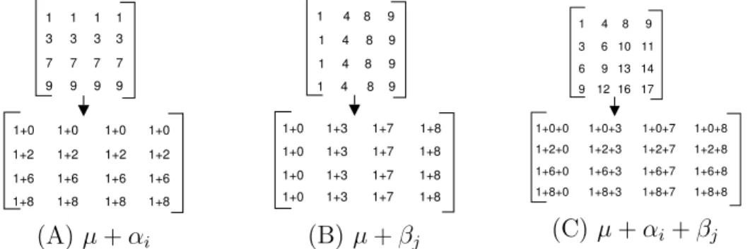
As an alternative to measures of distance, “conceptual” measures of similar-ity can be used. Models are based on constant rows, columns and coherent values, (additive or multiplicative), [10] (Fig. 1). A “good fit” indicates high correlation within a sub-matrix, (thus a possible cluster). These models are common to several clustering algorithms. For example, Cheng and Church [15] and FLOC [16], use the additive model (Fig. 1(C)), to evaluate biclus-ters obtained by determining the Mean Residue Score. Given a GE matrixA, the residue of an element aij in a sub-matrix (I, J) is given by the difference
rij = (aij−aiJ −aIj +aIJ), where aij, aiJ, aIj and aIJ are the sub-matrix
value, the row, column and group mean respectively. The “H-score” of the sub-matrix is then the sum of the residues, given by:
H(I, J) = 1
|I ||J |Σi∈Ij∈J(rij)
2 (1)
A perfect bi-cluster gives a H-score equal to zero, (corresponding to “ideal” GE data, with constant additive matrix rows and columns).
The Plaid Model [17] bi-cluster variant builds the GE matrix as a sum of layers, where each layer corresponds to a bi-cluster. Each valueaij is modelled
by aij = K X k=0
θijkρikκjk where K is the layer (bi-cluster) number, and ρik and
κjk are binary variables representing membership of row i and column j in
1 1 1 1 3 3 3 3 7 7 7 7 9 9 9 9 1+0 1+0 1+0 1+0 1+2 1+2 1+2 1+2 1+6 1+6 1+6 1+6 1+8 1+8 1+8 1+8 (A) µ+αi 1 1+0 1+0 1+0 1+0 4 8 9 1 4 8 9 9 9 1 1 4 4 8 8 1+3 1+3 1+3 1+3 1+7 1+7 1+7 1+7 1+8 1+8 1+8 1+8 (B) µ+βj 1 1+0+0 1+2+0 1+6+0 1+8+0 4 8 9 1+0+3 1+2+3 1+6+3 1+8+3 1+0+7 1+2+7 1+6+7 1+8+7 1+0+8 1+2+8 1+6+8 1+8+8 3 6 10 11 6 9 13 14 9 12 16 17 (C) µ+αi+βj
Fig. 1. Models for bi-clusters: (A) Bi-cluster with constant rows. Each row is ob-tained from a typical value µand row offsetαi, (B) Constant columns. Each value
is obtained from a typical value µand column offset βj, (C) Additive model. Each
value is predicted from µ, and a row and column offset, αi +βj. Similar model
constructs apply for the multiplicative case with (A(i)) µ×αi, (B(i)) µ×βj and
(C(i)) µ×αi×βj
function of the contributions of the different bi-clusters to which the row i
and the column j belong, (Fig. 2),[17]. For layer k, expression level θijk can
be estimated using the general additive model,θijk =µk+αik+βjk, in layer
k, (Fig. 1 (C)). 5 2 4 5 9 6 8 9 11 8 10 11 12 9 11 12 0 -3 -1 0 0 4 6 7 1 4 8 9 3 6 10 11 6 9 19 17 9 12 25 23 11 8 4 5 8 9 10 11 12 9 11 12 19=1+6+7+5+0+0 17=1+6+8+5+0-3 25=1+8+7+5+4+0 23=1+8+8+5+4-3 = 1 1 4 8 9 3 6 10 11 7 10 14 15 9 12 16 17 0 3 7 8 0 2 6 8 = 5
Fig. 2. Plaid Model GE values at overlaps are seen as a linear function of different bi-clusters.
For theCoherent Evolutions modelthe exact values ofxijare not directly taken
into account, but a cluster is evaluated to see if it shows coherent patterns of expression. In simplest model form, each GE value can have three states: up-regulation, down-regulation and no change. Thresholds between states are crucial and additional complexity results from extending model definitions to include further states such as “slightly” up-regulated, “strongly” up-regulated and so on, e.g. SAMBA [18].
Other measures used to evaluate coherency of a group of genes include condi-tional entropy:H(C|X) =−R
m X j=1
p(cj|x)logp(cj|x)p(x)dx(the average
uncer-tainty of the random variableC (cluster category), when a random variableX
when this entropy is minimised i.e. a partition where each gene is assigned with a high probability to only one cluster, [19]. This requires the estimation of the a posteriori probabilities p(cj|x), usually by non-parametric methods,
as this avoids assumptions on the distribution of the underlying GE data), [19].
Pattern proximity measures described so far make no distinction between time-series data and those obtained from expressions of two or more phenotypes. Applying similarity measures to time series data is not straightforward. Gene expression time series have non-uniform intervals and are usually very short (4-20 samples while classically even 50 observations is low for statistical infer-ence), further data are not independently, identically distributed data. Sim-ilarity in time series should be viewed only in terms of similar patterns in the direction of change across time points, while robust measures must allow for non-uniformity, in addition to scaling and shifting problems, and shape (internal structure of clusters), [20].
Each algorithm described below by definition, relies on some choice of prox-imity measure and inherits the limitations of that choice.
2.2 Agglomerative clustering
All agglomerative techniques naturally form a hierarchical cluster structure in which genes have a crisp membership. Eisen et al. [11] studied GE in the bud-ding yeast, Saccharmyces Cerevisiae, using hierarchical methods which have been popularised due to ease of implementation, visualisation capability and availability. Methods vary with respect to choice of distance metric, decision on cluster merging, (linkage), as well as parameter selection affecting struc-ture and relationship between clusters. Options include:single linkage (cluster separation as distance between two nearest objects), complete linkage (as pre-viously, but between two furthest objects), average linkage (average distance between all pairs), centroid (distance between centroid’s of each cluster) and Ward’s method, (which minimises ANOVA Sum of Squared Errors between two clusters)[21].
Distance and linkage determine level of sensitivity to noise: Ward’s and Com-plete method are particularly affected, (due to the ANOVA basis and out-lier importance respectively, since clustering decisions depend on maximum distance between two genes). Single linkage forces cluster merger, based on minimum distance, regardless of other gene contributions to the cluster, so noisy or outlying values are among the last to be considered. Consequently, the “chaining phenomenon” may arise, [13]. For commonly used Average and Centroid linking this problem is avoided as no special consideration is given
to outliers and clusters are based on highest density.
Results for agglomerative clustering may be intuitively presented by dendo-grams but there are 2n−1 different linear orderings consistent with tree
struc-ture, so care is needed in pruning. Dendrogram analysis, based on gene class information from specialised databases is presented in [22], where optimal correlations are obtained between gene classes and used to form clusters from different branch lengths. In [23] authors present an agglomerative technique for which each internal node has at most N children, allowing up toN genes (or clusters) to be directly connected, (extending traditional hierarchical concepts and reducing the effects of noise). Permutation is used to decide on the num-ber of nodes (maxN) to merge, based on a similarity threshold. Heuristically, algorithm complexity is comparable to traditional hierarchical clustering, [23], although the authors also present a “divide and conquer” approach for opti-mal leaf ordering for sopti-mall N, which has implications of increased time and space complexity.
It should be stated that, such methods can not, in general, compensate for the greedy nature of the traditional algorithm, where mis-clustering at the beginning can not be corrected at a later stage and are magnified as the process continues. Further, [24] and [25] note that hierarchical clustering performance is close to random, despite its popularity and is poorer than other common techniques such as K-means and Self Organising maps (SOM).
2.3 Partitive Techniques
Partitive clustering divides data by similarity measure, where typical methods measure distance from a gene vector to a prototype vector representing the cluster, and intra-cluster/inter-cluster distance are respectively maximised and minimised. A major drawback is the need to specify the number of clusters in advance. Table 2 summarises algorithms discussed here.
K-means produces crisp clusters with no structural relationship between these, [26]. It deals poorly with noise, since outliers must belong to a cluster and this distort the means. Equally, cluster inclusion is dependent on the cumula-tive values of genes already present, soorder matters. Results are dependent on initial cluster prototype (which varies between clustering attempts); this leads to instability and, frequently, to a local minimum solution. Incremental approaches to refine local minima solutions close towards a global solution, include the Modified Global K-means (MGKM) algorithm [27], which com-putes k-partitions of the data using k −1 clusters from previous iterations. A tolerance threshold must be set which determines the number of clusters indirectly, and, as with regular K-means, returns spherical clusters. For the
six datasets reported [27], the MGKM algorithm showed slight improvement over K-means, but at higher computational time cost.
The prevalence of local minima for K-means is linked to initial prototype selection. Genetic algorithms (GAs), as an evolutionary approach, work well for small datasets, (less than 1000 gene vectors and of low dimension), but have prohibitive time constraints for anything larger, so are less desirable for GE analysis. Although GA’s find the global optimum, they are sensitive to user defined input parameters and must be fine tuned for each specific problem. Studies which have combined K-means and GA include Incremental Genetic K-Means Algorithm (IGKA), [28]. This is a hybrid approach which converges to a global optimum faster than stand alone GA, and without the sensitivity to initialisation prototypes. The fitness function for the GA is based on Total Within Cluster Variance (TWCV), while the basis of the algorithm is to cluster centroids incrementally, using a standard similarity measure. The GA method requires the number of output clusters, K, to be specified, but is further complicated by inherent GA parameters (mutation probability rate, number of generations, size of the chromosome populations etc.), which influence time taken by the algorithm to converge to a global optimum.
Fuzzy modifications of K-means includeFuzzy C-Means (FCM)[29] and Fuzzy clustering by Local Approximations of MEmberships (FLAME) [30]. In both, genes are assigned a cluster membership degree indicating percentage associ-ation with that cluster, but the two algorithms differ in the weighting scheme used to determine gene contribution to the mean. For a given gene, FCM membership value of a set of clusters is proportional to its similarity to clus-ter mean. The contribution of each gene to the mean of a clusclus-ter is weighted, based on its membership grade. Membership values are adjusted iteratively until the variance of the system falls below a threshold. These calculations require the specification of a degree of fuzziness parameter which is problem specific [29]. As with K-Means, clusters are unstable, and considerably in-fluenced by initial parameter values, while K, the number of clusters, must be specified a priori. In contrast FLAME requires membership of a cluster,
i, to be determined by the weighted similarity of the gene to its K-nearest neighbours, and their membership of cluster i. This density-based approach further reduces noise impact, since genes with a density lower that a pre-defined threshold are categorised as outliers, and grouped with a dedicated ‘outlier’ cluster. FLAME produces stable clusters, but the size of the neigh-bourhood and the weighting scheme used affect K (as above) and clustering achieved. For both FCM and FLAME, genes may have multiple and varied degrees of membership, but interpretation differs. FCM and FLAME use av-eraging, where each gene contributes to the calculation of a cluster centroid, and its overall membership value set sums to 1, (i.e. gene-cluster probability). Thus strong membership for a given gene does not indicate it to be more typical of the cluster, but rather relative strength of its individual association,
GID Cluster 4 Cluster 21 Cluster 46
Centroid Dist. Mem. Centroid Dist. Mem. Centroid Dist. Mem.
A 10.691 0.002575 8.476 0.002002 3.864 0.482479
B 6.723 0.009766 3.855 0.009341 6.33 0.007381
C 6.719 0.007653 5.29 0.00515 8.024 0.005724
D 7.725 0.007609 3.869 0.01782 6.279 0.010249
Table 1
Membership of a gene and distance to cluster centroid, as calculated by Euclidean distance.
[31].
Table 1 illustrates for three clusters. For FCM carried out on published yeast genomic expression data [32], results are available at http://rana.lbl.gov/ FuzzyK/data.html. Membership values for genes B and D are very different for cluster 21, although both are approximately equidistant from the centroid of the cluster. Similarly genes C and D have comparable membership values for cluster 4, but gene C is more typical (closer to the centroid) than gene D. With similar centroid distances, membership values for gene B in cluster 21 is smaller than that of gene A in cluster 46. These anomalies arise from the membership sum constraint, which decreases gene membership in one cluster to increase it in another. Listing genes in a cluster based on membership val-ues is therefore counter-intuitive and does not reflect their compatibility with the cluster, but rather how they are shared between clusters. Similarly for FLAME, as the memberships are weighted relative to the K-nearest neigh-bours, so a low membership value indicates a high degree of cluster sharing among these and not a more typical value og a given cluster. This interpre-tative flaw was recognised by [33], who developed the possibilistic biclustering algorithm, which removes the sum rule restriction. The authors used spectral clustering principles [34] to create from the original GE matrix, a partition matrix, Z, to which possibilistic clustering is applied. The resulting clusters were evaluated using the H-Score, (Eq.1), and improved on traditional tech-niques. The algorithm requires, inter alia, two specific parameters, namely cutoff membership for (i) gene inclusion and a(ii) sample inclusion in a clus-ter. In this case, these cutoffs are intuitively reasonable as membership does indicate how typical a gene/sample is to a defined cluster, andnot the degree to which it is shared between clusters.
2.4 Neural Networks
Neural Networks (NN), loosely based on the biological parallel, can be mod-elled as a collection of nodes with weighted interconnections. Only numerical vectors are processed, so meta-information can not be included in the cluster-ing procedure. Interconnection weights areadaptively learned i.e. features are
Cluster Mem. Input Proximity Other
K-Means Hard Starting Proto- Pairwise Very Sensitive types, Stopping Distance to input parameters
Threshold, K and order of input.
MGKM Hard Tolerance Thres- Pairwise Not as sensitive to
hold Distance starting prototypes.
K specified through tolerance threshold.
IGKA Hard K, mutation prob. TWCV Time taken to
generation number, converge to global
population size influenced by parameters.
FCM Fuzzy Degree of fuzzi- Pairwise Careful Interpretation
ness, Starting Distance of membership values.
prototypes, Stop Sensitive to input
para-threshold, K metres and order of input.
FLAME Fuzzy Knn- Pairwise careful interpretation
number of Distance of membership
neighbours toKnn values. Output
neighbours determined byKnn.
Possibilistic Fuzzy Cut-off memberships H-Score Number of biclusers
biclustering Max. residue, number of rows determined when quality and number of columns function peaks by
re-running for different numbers of eignevalues. Table 2
Summary of Partitive techniques. With the exception of FLAME and Possibilistic biclustering, all find complete global clusters.
selected by appropriate assignment of weights. In particular, Self Organising Maps (SOMs), a type of NN, have proved popular for GE, [12, 35, 36]. A kernel function, that defines the region of influence, (neighbourhood), for an input gene, distinguishes SOM from K-means. Updating the kernel function causes the output node and its neighbours, to track towards the gene vector. The network is trained, (adjusting strengths of interconnections), from a ran-dom sample of the dataset. Once training is complete, all genes in the dataset are then applied to the SOM. Cluster members, represented by output nodei
are the set of genes causing i to ‘fire’ (hard clustering).
SOMs are robust to noise and outliers, dependent on distance metric and neighbourhood function used. As for K-means, a SOM produces a sub-optimal solution if the initial weights for the interconnections are not chosen properly. Convergence is controlled by problem-specific parameters such aslearning rate and neighbourhood function. A particular input pattern can fire different out-put nodes at different iterations; )while this can be overcome by gradually reducing the learning rate to zero during training, it can result in over-fitting,
which leads to poor performance for new data). In specifying K, based on the number of output nodes, it should be noted that too few output nodes in the SOM gives large within-cluster distance, while too many results in meaningless diffusion.
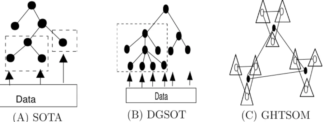
The Self Organizing Tree Algorithm (SOTA) [37], Dynamically Growing Self Organizing Tree (DGSOT)algorithm [38] and, more recently,Growing Hierar-chical Tree SOM (GHTSOM)[39] were developed to combine strengths of NN (i.e. speed, robustness to noise) and hierarchical clustering (i.e. tree structure output, minimum a priori requirement for number of clusters specification and training) to deal with properties of GE data. Here the SOM network is a tree structure, trained by comparing only leaf nodes to input GE profiles (each graph node represents a cluster). SOTA and DGSOT result in a binary and n-tree structure respectively, while in GHTSOM, each node is a trian-gular SOM (3 neurons, fully connected), each having 3 daughter nodes (also triangular SOMs), Fig. 3. Tree growth strategy determines K. At each itera-tion of SOTA the leaf node with the highest degree of heterogeneity is split into two daughter cells. In the DGSOT case, the correct number of daughters, (nd ≥ 2), is determined dynamically by starting off with two and
continu-ally adding one until cluster validation criteria are satisfied. To determine nd,
a method was proposed [38], based on geometric characteristics of the data (specifically, cluster separation in the minimum spanning tree of the cluster centroids). For this an empirical threshold, α, value must be specified; (the authors propose 0.8)). In SOTA and DGSOT, growth of the tree continues until overall heterogeneity crosses a threshold, β, or until all genes map onto a unique leaf node. The DGSOT method uses average leaf distortion to deter-mineβ for growth termination. While, for SOTA, this threshold is determined by re-sampling, with system variability defined to be the maximum distance among genes mapped to the same leaf node. By comparing distances between randomized data and those of the real dataset, a confidence interval and dis-tance cut-off are obtained. In GHTSOT, growth occurs if a neuron is activated if a sufficient number of inputs map to it, (i.e. at least 3 or a user defined num-ber, β) which determines the resolution of the system. Growth continues as long as there is one neuron in the system which can grow. The advantage of these methods over most partitive techniques is thatK is not pre-determined, but depends indirectly on the threshold, β, which is data dependant.
SOTA, DGSOT and GHTSOM differ from typical hierarchical clustering al-gorithms in terms of adaption. This occurs once a gene is mapped to a leaf node, but the neighbourhood of the adaptation is more restrictive than for SOM. DGSOT also overcomes the misclustering problem of the traditional hi-erarchical algorithm, SOTA and GHTSOM, by specification of another input parameter,L - the immediate ancestor level in the tree of a given node which is growing. DGSOT then distributes all mapped values among the leaves of the subtree rooted at theLthancestor. In GHTSOM, new nodes (after growth)
Structure Proximity Input Other
SOM None Distance number of Careful consideration
output neurons, of initalisation weights Learning rate
SOTA Binary Tree Distance Thresholdβ
DGSOT N-ary Tree Distance Thresholdsβ,α Corrects for
andL. misclusterings
GHTSOM Each node Distance Minimal requirement triangular SOM, arranged - learning rate in Tree structure
Table 3
Summary of Neural Network techniques presented.
are trained using only those inputs which caused the parent node to fire. Any neuron, which shows low activity, is deleted, and its parent is blocked from further growth. This has the advantage that inputs mapping to leaf neurons at the top of the hierarchy are usually noise, and clearly distinguishable from relevant biological patterns.
Data
(A) SOTA
Data
(B) DGSOT (C) GHTSOM
Fig. 3. Self-Organising tree structures: (A) SOTA. A binary tree structure. Neigh-bourhood of adaption indicated for (i) node with sibling, (ii) node with no sib-ling, (B) DGSOT. N-ary tree structure. Neighbourhood of adaption indicated when
L= 2, (C) GHTSOM. Each node represented by triangular SOM. Each layer indi-cated with line styles, (3 layers shown).
2.5 Search Based
Solutions for a criterion function are found by searching the solution space either deterministically or stochastically [3]. The former exhaustive search is of little use for high dimensional GE analysis and, typically, heuristics are used. Simulated Annealing is well-known and has been applied [40] using TWCV to minimise the fitness function, E, and, [41],by minimising H-Score (Eq. 1). At each stage of the process, gene vectors are randomly chosen and moved to a new random cluster. E is evaluated for each move and the new assignment
is accepted if E is improved or with a probability of e−Enew−Eold
T otherwise.
The “temperature”, T, controls readiness of the system to accept the poorer situation by chance, enabling the algorithm to avoid local minima. As the search continues, T, is gradually reduced according to an annealing schedule, and ultimately achieves the global minimum, where the annealing schedule parameters dictate performance and speed of the search. Choice of initial Ti
governs convergence time and size of search space, (increased/decreased in the case of high/low T respectively). Similarly for search termination, (final effective TF). The user must specify the rate at whichT approachesTF, which
must be slow enough to guarantee a global minimum, as well as the number of swaps of gene vectors between clusters allowed in an iteration.
To determineK, a randomisation procedure is used, [40], to determine cut-off threshold for the distance, D, between two gene vectors in a single cluster. It is also necessary to determine P, the probability of accepting false positives, (e.g. P = 0.05). Simulated annealing is then applied for different numbers of clusters, until the weighted average fraction of incorrect gene vector pairs reaches the P-value.
The algorithm of Cheng and Church [15] (adapted from Hartigan [42]) ob-tains H-scores, (Eq. 1, Fig. 1) [10]) of the sub-matrices of the GE matrix. This method is initialised for the entire GE matrix and considers a sub-matrix to be a bi-cluster ifH(I, J)< δ for someδ ≥0, (user defined). Each row and column of the original matrix is thus tested for deletion. Once a sub-matrix is deter-mined to be a bi-cluster, its values are “masked” with random numbers in the initial GE matrix. Masking bi-clusters prevents the algorithm from repeatedly finding the same sub-matrices, but there is a substantial risk that this replace-ment will interfere with the discovery of future bi-clusters, [16]. To overcome this problem of random interference,Flexible Overlapped biClustering (FLOC) was developed - a generalised model of Cheng and Church incorporating null values, [16]. FLOC constrains the clusters to both a low mean residue score and a minimum occupancy threshold of α, 0 ≤ α ≤ 1 (user defined). Note: this method does not require pre-processing for imputation of missing values. Both, these bi-clustering algorithms find coherent groups (Section 2.1) in the data and permit overlapping.
The Plaid Model [17] (Section 2.1) assumes that bi-clusters can be generated using a statistical model and aims to identify the parameter distribution that best fit the available data, by minimising the error sum of squares for the
kth bi-cluster assuming that k − 1 bi-clusters have already been identified.
Explicitly, it seeks to minimise for the whole matrix: Q = 12
n X i=1 m X j=1 (Zij −
Proximity Deterministic/ Clusters Other Stochastic
SA Depends on Stochastic Depends on Specification of
application application Annealing Schedule
CC Additive Model Deterministic Overlapping, partial δ,
bi-clusters random interference
FLOC Additive Model Deterministic Overlapping, partial αandδ
bi-clusters to specify. Overcomes random interference, allows missing values.
Plaid Additive Model Deterministic Overlapping, partial Values seen as sum of bi-clusters contributions to bi-clusters Table 4
Summary of search based techniques presented.
(Zij =aij− KX−1
k=0
θijkρikκjk). Parametersθijk,ρik andκjk are estimated for each
layer and for each value in the matrix, and are updated iteratively, providing refined estimates of µk, αik and βjk, (Fig: 1(C)) and ρik and κjk to minimise
Q, [17].
The importance of a layer is defined byδ2
k = Pn
i=1
Pp
j=1ρikκjkθ2ijk. To evaluate
the significance of the residual matrix, Z is randomly permuted and tested for importance. If δk2 is significantly better than δrandom2 , k is reported as a
bi-cluster. The algorithm stops when the residual matrixZ retains only noise, with the advantage that the user does not need to specify the number of clusters beforehand.
2.6 Graph Theoretic Methods
Graph theoretic approaches have recently gained ground in analysing large complex datasets. The Cluster Affinity Search Technique (CAST), [43], mod-els data as an undirected graph, G = (V, E), where {V, E} is the set of
{vertices, edges}representing{genes, similarexpression}. The model assumes that there is an ideal clique graph, (a disjoint union of complete sub-graphs),
H = (U, E), which represents the ideal input gene expression dataset, while data to be clustered is a “contamination” of the ideal graph H by random errors. In a clique graph each clique represents a cluster. For a pair of genes in
G, the model assumes that an edge/non-edge was assigned incorrectly, with a probability of α. The true clustering of G is assumed to be that which re-quires fewer edge changes to generate H. CAST uses an affinity (similarity) measure, either binary or real valued, to assign a vertex to a cluster. Affin-ity to a cluster must be above a threshold, t (user defined which determines size and number of clusters). The affinity of a vertex v to a cluster, is the
sum of affinities over all objects currently in the cluster, so v has high affinity with i if af f inity(x) > t|i|, and low affinity otherwise. The CAST algorithm alternates between adding high affinity elements and removing low affinity elements, finding clusters one at a time. The result is dependent on the order of input as once initial cluster structure is obtained, a vertex v is moved to that cluster for which it has a higher affinity value.
CLICK [44], builds on the work of [45], which uses a probabilistic model for edge weighting. Pairwise similarity measures between genes are assumed to be normally distributed: between ‘mates’ (N(µT, σT2)), and between
‘non-mates’ (N(µF, σF2)), where µT > µF. These parameters can be estimated
via Expectation Maximisation methods [46]. The weight of an edge is de-rived from the similarity measure between the two gene vectors, and re-flects the probability that i(∈ V) and j(∈ V) are mates, specifically that:
wij = log(1−pmatespmates)σFσT +
(Sij−µF)2 2σ2
F −
(Sij−µT)2 2σ2
T . Edges with weights below a user
defined non-negative threshold are omitted from the graph. The graph is par-titioned using a minimum weight cut algorithm [45].
TheStatistical Algorithmic Method for Bi-cluster Analysis (SAMBA) method finds bi-clusters based on the coherent evolution model (Section 2.1) [18]. Firstly, the gene expression matrix is modelled as a bipartite graph, G = (U, V, E), where U is the set of sample vertices, U ∩ V = ∅ and an edge
(u, v) only exists between v ∈ V and u ∈ U iff there is a significant change in expression level of gene v, w.r.t. to its normal level, in sample u. Key to SAMBA is the scoring scheme for a bi-cluster, corresponding to its statistical significance, where a weight is assigned to a given edge, (u, v), based on the log-likelihood of getting that weight by chance [18], (log Pc
P(u,v) > 0 for edges
and, log(1(1−P−(u,v))Pc) < 0 for non-edges). The probability P(u,v) is the fraction of
random bipartite graphs, with degree sequence identical to G, that contain edge (u, v) (and can be estimated using Monte-Carlo methods). Pc is a
con-stant probability > max(u,v)∈U xVP(u,v). Assigning these weights to the edges
and non-edges in the graph, the statistical significance of a subgraph H can be calculated, and the K heaviest (largest weight) sub-graphs for each vertex inG found. The authors, [18] present two ways to calculate the weight of the resulting sub-graph. In the simpler model, bi-clusters, which reflect changes relative to normal expression level, without considering direction of change are sought. The second model, focuses onconsistent bi-cliques, targeting those samples which have the same or opposite effect on each of the genes.
Mode Proximity Search Other
CAST One Mode Similarity Clique Parametersαandt. Finds global, Graph complete, crisp clusters.
CLICK One Mode Distribution Minimum Stat. Sig. of clusters. EM to based on weight cut estimate parameters. Finds distance global, partial, crisp clusters.
SAMBA Bi-Partite Probability Heuristic Stat. sig. of clusters. Input search of Pcdifficult to define. Finds neighbours partial overlapping bi-clusters. Table 5
Summary of performance criterion of Graph theoretic methods presented.
3 Discussion
Despite shortcomings, application of clustering methods to GE data has proven to be of immense value, providing insight on cell regulation, as well as on disease characterisation. Nevertheless, not all clustering methods are equally valuable for high dimensional GE data. Recognition that well-known, simple clustering techniques, such as K-Means and Hierarchical clustering, do not capture complex local structure, has led to investigation of other options. In particular, bi-clustering has gained considerable recent popularity. Indications to date are that these methods provide increased sensitivity at local structure level in discovery of meaningful biological patterns.
An inherent problem with exploratory clustering isab initio knowledge ofK, the number of clusters. Consequently, those methods for GE analysis which do not need K specified ab initio have an advantage. Most algorithms seek em-pirically to determine this at run time, but derive complicated thresholds that may not make sense in the context of gene expression data. There is a risk that determination of these thresholds is not a one step process but requires testing and validation of clusters produced. While space limits a comprehensive sur-vey of robust cluster validation and evaluation methods here, their importance is clear: (see [47] for a comprehensive review). A discipline of information-driven clustering is emerging, which integrates cluster and meta-information, [48, 49, 50, 51, 52]. These provide a basis for validation, independent of the current problem and simplify interpretation of clustering results.
4 Conclusion
Cluster analysis applied to GE data aims to highlight meaningful patterns for gene co-regulation. The evidence suggests that, while commonly applied, ag-glomerative and partitive techniques are insufficiently powerful given the high dimensionality and nature of the data. While further testing on non-standard
and diverse data sets is required, comparative assessment and numerical evi-dence, to date, supports the view that bi-clustering methods, although com-putationally expensive, offer better interpretation in terms of data features and local structure. While the limitations of commonly-used algorithms are well documented in the literature, adoption by the bioinformatic community of new (and hybrid) techniques developed specifically for GE analysis has been slow , mainly due to the increased algorithmic complexity required. This would be catalysed by more transparent guidelines and increased availability in specialised software and public dataset repositories.
References
[1] M. H. Asyali, D. Colak, O. Demirkaya, and M. S. Inan. Gene expression profile classification: A review. Curr. Bioinformatics, 1(1):55–73, 2006. [2] T. D. Pham, C. Wells, and D. I. Crane. Analysis of microarray gene
expression data. Curr. Bioinformatics, 1(1):37–53, 2006.
[3] A. K. Jain, M. N. Murty, and P. J. Flynn. Data clustering: A review. ACM CSUR, 31(3):264–323, 1999.
[4] S. O. Zakharkin, K. Kim, T. Mehta, L. Chen, S. Barnes, K. E. Scheirer, R. S. Parrish, D. B. Allison, and G. P. Page. Sources of variation in affymetrix microarray experiments. BMC bioinformatics, 6:214, Aug 29 2005.
[5] O. Troyanskaya, M. Cantor, G. Sherlock, P. Brown, T. Hastie, R. Tibshi-rani, D. Botstein, and R. B. Altman. Missing value estimation methods for dna microarrays. Bioinformatics, 17(6):520–525, Jun 2001.
[6] X. Liu, G. Cheng, and J. X. Wu. Analyzing outliers cautiously. IEEE Trans. Knowl. Data Eng., 14(2):432–437, 2002.
[7] G. W. Milligan and M. C. Cooper. An examination of procedures for determining the number of clusters in a dataset. Psychometrika, 50:159– 179, 1985.
[8] J. Fridlyand and S. Dudoit. Applications of resampling methods to esti-mate the number of clusters and to improve the accuracy of a clustering method. Technical Report 600, Department of Statistics, University of California, Berkeley, 2001.
[9] A. Ben-Dor, B. Chor, R. Karp, and Z. Yakhini. Discovering local struc-ture in gene expression data: the order-preserving submatrix problem. J. Comput. Biol., 10(3-4):373–384, 2003.
[10] S. C. Madeira and A. L. Oliveira. Biclustering algorithms for biological data analysis: a survey. IEEE/ACM Trans. Comput. Biol. Bioinform., 1(1):24–45, 2004.
[11] M. B. Eisen, P. T. Spellman, P. O. Brown, and D. Botstein. Cluster analysis and display of genome-wide expression patterns. Proc. Natl. Acad. Sci USA, 95(25):14863–14868, Dec 8 1998.
[12] T. Kohonen. The self-organizing map. Proceedings of the IEEE, 78(9):1464–1480, 1990.
[13] C. Romesburg. Cluster Analysis for Researchers. Lulu Press, Morrisville, 2004.
[14] D. W. Kim, K. H. Lee, and D. Lee. Detecting clusters of different geometrical shapes in microarray gene expression data. Bioinformatics, 21(9):1927–1934, May 1 2005.
[15] Y. Cheng and G. M. Church. Biclustering of expression data. ISMB ’00, 8:93–103, 2000.
[16] J. Yang, H. Wang, W. Wang, and P. Yu. Enhanced biclustering on ex-pression data. BIBE ’03, page 321, 2003.
[17] L. Lazzeroni and A. B. Owen. Plaid models for gene expression data. Statistica Sinica, 12(1):61–86, 2000.
[18] A. Tanay, R. Sharan, and R. Shamir. Discovering statistically significant biclusters in gene expression data. Bioinformatics, 18 Suppl 1:S136–44, 2002.
[19] H. Li, K. Zhang, and T. Jiang. Minimum entropy clustering and appli-cations to gene expression analysis. Proc. IEEE CSB., pages 142–151, 2004.
[20] C. Moller-Levet, K. H. Cho, H. Yin, and O. Wolkenhauer. Clustering of gene expression time-series data. Technical report, 2003.
[21] A. Sturn. Cluster analysis for large scale gene expression studies, 2001. [22] P. Toronen. Selection of informative clusters from hierarchical cluster tree
with gene classes. BMC bioinformatics, 5:32, Mar 25 2004.
[23] Z. Bar-Joseph, E. D. Demaine, D. K. Gifford, N. Srebro, A. M. Hamel, and T. S. Jaakkola. K-ary clustering with optimal leaf ordering for gene expression data. Bioinformatics, 19(9):1070–1078, Jun 12 2003.
[24] K. Y. Yeung, D. R. Haynor, and W. L. Ruzzo. Validating clustering for gene expression data. Bioinformatics, 17(4):309–318, Apr 2001.
[25] F. D. Gibbons and F. P. Roth. Judging the quality of gene expression-based clustering methods using gene annotation. Genome Res., 12(10):1574–1581, Oct 2002.
[26] J. B. MacQueen. Some methods for classification and analysis of multi-variate observations. In L. M. Le Cam and J. Neyman, editors,Proc. Fifth Berkeley Symp. Math. Stat. Prob., pages 281–297. University of California Press, 1967.
[27] Adil M. Bagirov and Karim Mardaneh. Modified global k-means algo-rithm for clustering in gene expression data sets. In WISB ’06, pages 23–28, Darlinghurst, Australia, 2006. Australian Computer Society, Inc. [28] Y. Lu, S. Lu, F. Fotouhi, Y. Deng, and S. J. Brown. Incremental genetic
k-means algorithm and its application in gene expression data analysis. BMC bioinformatics, 5:172, Oct 28 2004.
[29] D. Dembele and P. Kastner. Fuzzy c-means method for clustering mi-croarray data. Bioinformatics, 19(8):973–980, May 22 2003.
analysis of dna microarray data. BMC bioinformatics, 8:3, Jan 4 2007. [31] R. Krishnapuram and J. M. Keller. A possibilistic approach to clustering.
IEEE TFS, 1(2):98–110, 1993.
[32] A. P. Gasch and M. B. Eisen. Exploring the conditional coregulation of yeast gene expression through fuzzy k-means clustering. Genome biology, 3(11):RESEARCH0059, Oct 10 2002.
[33] C. Cano, L. Adarve, J. Lopez, and A. Blanco. Possibilistic approach for biclustering microarray data. Comp. Biol. Med., 37(10):1426–1436, Oct 2007.
[34] Y. Kluger, R. Basri, J. T. Chang, and M. Gerstein. Spectral biclustering of microarray data: coclustering genes and conditions. Genome Res., 13(4):703–716, Apr 2003.
[35] P. Tamayo, D. Slonim, J. Mesirov, Q. Zhu, S. Kitareewan, E. Dmitrovsky, E. S. Lander, and T. R. Golub. Interpreting patterns of gene expression with self-organizing maps: methods and application to hematopoietic dif-ferentiation. Proc. Natl. Acad. Sci. USA, 96(6):2907–2912, Mar 16 1999. [36] T. R. Golub, D. K. Slonim, P. Tamayo, C. Huard, M. Gaasenbeek, J. P. Mesirov, H. Coller, M. L. Loh, J. R. Downing, M. A. Caligiuri, C. D. Bloomfield, and E. S. Lander. Molecular classification of cancer: class discovery and class prediction by gene expression monitoring. Science, 286(5439):531–537, Oct 15 1999.
[37] J. Herrero, A. Valencia, and J. Dopazo. A hierarchical unsupervised growing neural network for clustering gene expression patterns. Bioin-formatics, 17(2):126–136, Feb 2001.
[38] F. Luo, L. Khan, F. Bastani, I. L. Yen, and J. Zhou. A dynamically grow-ing self-organizgrow-ing tree (dgsot) for hierarchical clustergrow-ing gene expression profiles. Bioinformatics, 20(16):2605–2617, Nov 1 2004.
[39] A. Forti and G. L. Foresti. Growing hierarchical tree som: an unsupervised neural network with dynamic topology. Neural networks, 19(10):1568– 1580, Dec 2006.
[40] A. V. Lukashin and R. Fuchs. Analysis of temporal gene expression profiles: clustering by simulated annealing and determining the optimal number of clusters. Bioinformatics, 17(5):405–414, May 2001.
[41] K. Bryan, P. Cunningham, and N. Bolshakova. Application of simu-lated annealing to the biclustering of gene expression data. IEEE T-ITB, 10(3):519–525, Jul 2006.
[42] J. A. Hartigan. Direct clustering of a data matrix. JASA, 67(337):123– 129, 1972.
[43] A. Ben-Dor, R. Shamir, and Z. Yakhini. Clustering gene expression pat-terns. J. Comput. Biol., 6(3-4):281–297, Fall-Winter 1999.
[44] R. Sharan and R. Shamir. Click: a clustering algorithm with applications to gene expression analysis. ISMB ’00, 8:307–316, 2000.
[45] E. Hartuv, A. O. Schmitt, J. Lange, S. Meier-Ewert, H. Lehrach, and R. Shamir. An algorithm for clustering cdna fingerprints. Genomics, 66(3):249–256, Jun 15 2000.
[46] A. P. Dempster, N. M. Laird, and D. B. Rubin. Maximum likelihood from incomplete data via the em algorithm. J Royal Statistical Soc B (Methodological), 39(1):1–38, 1977.
[47] J. Handl, J. Knowles, and D. B. Kell. Computational cluster validation in post-genomic data analysis. Bioinformatics, 21(15):3201–3212, Aug 1 2005.
[48] G. Gamberoni, S. Storari, and S. Volinia. Finding biological process modifications in cancer tissues by mining gene expression correlations. BMC Bioinformatics, 7(6):8, Jan 9 2006.
[49] R. Kustra and A. Zagdanski. Incorporating gene ontology in clustering gene expression data. CBMS, 0:555–563, 2006.
[50] J. Kasturi and R. Acharya. Clustering of diverse genomic data using information fusion. Bioinformatics, 21(4):423–429, 2005.
[51] J.K. Choi, J.Y. Choi, D.G. Kim, D.W. Choi, B.Y. Kim, K.H. Lee, Y.I. Yeom, H.S. Yoo, O.J. Yoo, and S. Kim. Integrative analysis of multiple gene expression profiles applied to liver cancer study. FEBS Letters, 565(1-3):93–100, 2004.
[52] J. Liu, W. Wang, and J. Yang. Gene ontology friendly biclustering of expression profiles. In CSB ’04, pages 436–447, Washington, DC, USA, 2004. IEEE Computer Society.