Cooperative Random Walk for Pipe Network Layout Optimization
Stefan Ivić*Faculty of Engineering, University of Rijeka, Rijeka, Croatia. Luka Grbčić
Faculty of Engineering, University of Rijeka, Rijeka, Croatia. Siniša Družeta
Faculty of Engineering, University of Rijeka, Rijeka, Croatia.
Abstract
Pipe network layout optimization is an important and difficult problem in pipe network engineering. Differing from the previously proposed approaches for various optimization formulations, the authors use a methodology for pipe network optimization consisting of network layout optimization coupled with pipe sizing analysis. The methodology is based on a novel heuristic optimization algorithm inspired by Ant Colony Optimization, called Cooperative Random Walk (CRW). CRW successfully finds an optimal network layout for a range of pipe diameter values, as shown on a test base network of 40 nodes and 68 pipes with one source and 12 consumer nodes. The results clearly show how larger pipe diameters allow for simpler network layouts, while smaller pipe sizes automatically imply more complex and longer networks. Although CRW is tested on a water supply network problem, it is suitable for other network optimizations as well. Keywords: Cooperative Random Walk, Pipe Network Layout Optimization, Stochastic optimization method.
Introduction
Pipe network layout optimization is an important problem in water supply network engineering, as well as in pipe network engineering in general. Considering the often high installation cost of pipe networks, finding the most cost-effective pipe network configuration is necessary for achieving a long economic life of a pipe network.
Many authors have examined the concept of optimizing pipe networks, covering various approaches for solving optimization problems arising from different aspects of pipe network design, maintenance, control or operation. Pipe networks optimization problems, as well as optimization problems in general, are formulated by optimization variables, objectives and constraints. The overview of main types of pipe network optimizations is given in Table 1.
In this paper we deal with the problems of optimal design of pipe networks, which can be, according to past researches, classified as sizing optimization (i.e. pipe diameter optimization), network layout optimization, or pipe network layout and sizing optimization.
Unrelated to the type of optimization variables, different optimization objectives and optimization constraints are defining the optimal design of a pipe network. Most commonly used objective, which regulates the economic efficiency of a network, is the total cost of pipes. The hydraulic aspect of network design is mainly handled by different constraints: prescribed minimum pressure or minimum flow, network reliability etc.
Optimization of networks by sizing the pipes used in a predefined fixed network layout is the most commonly used type of pipe network design optimization. Pipe diameters can be considered as discrete optimization variables, which implies combinatorial optimization problem. This elementary characteristic of the optimization problem allows for the application of wide range of optimization methods so as to achieve optimal pipe sizing.
For solving combinatorial problem, where pipe diameters are chosen from a set of available values, a great number of various methods have been proposed: Simulated Annealing [2], Tabu Search [3], Genetic Algorithm [4, 1], Harmony Search [5], Shuffled Complex Evolution [6], Ant Colony Optimization [7, 8, 9], Particle Swarm Optimization [10], Soccer League Competition Algorithm [11] and Cross Entropy Optimization [12].
By allowing for the exclusion of pipes from the base network, the pipe sizing problem can be easily extended to network layout and sizing optimization. A "zero diameter" is added to the set of available diameters which can be used on every pipe in the base network. The pipe with "zero diameter" has no cost and there is no flow through that pipe, thus it can be considered as excluded from the pipe network. This raises a fundamental problem of possible network layouts which are topologically invalid, such as a network with a consumer node not connected to the source or a network with isolated pipes. The described layout and sizing formulation defines a similar optimization problem as pipe sizing, and is solved by several authors using different optimization techniques: Ant Colony Optimization [13, 14], Genetic Algorithm [15, 16] and hybrid optimization methods such as combination of Genetic Algorithm and Particle Swarm Optimization [17, 18].
Optimizing only the layout of a network, compared with pipe sizing or coupled pipe sizing and network layout, has not yet
been thoroughly researched. Fügenschuh et al. [19] combined mixed-integer linear programming, nonlinear optimization and constraint programming for optimization of gas distribution network. Another approach, using Ant Colony Optimization, is presented in [20, 21].
The optimization objective, in all reviewed papers, is to minimize the total cost of pipes, which depends on length and diameter of all pipes in the network. A minimal pressure requirement at each demand node is the most commonly used constraint. Some authors use additional constraints such as bounding velocity in pipes [8, 13, 9, 22, 16] or requiring a certain level of network reliability [13, 16, 21]. Hydraulic reliability of water distribution systems [23] is an important constraint in pipe network design, and, as it is shown in stated papers, can be relatively easily included in the network optimization method.
Table 1: Overview of pipe network optimization approaches [1] Optimization type Objective Possible variables Main constraints
Design Minimize cost Pipe layout; pipe diameters; pipe rehabilitation Min. level of service; available diameters; rehabilitation options; available budget; LCC Operation Minimize operational cost Pump controls; reservoir levels; sources and capacity Min. level of service; number of pump switches; source capacity; pump capacity Calibration Minimize difference between model and observed values Pipe roughness; pipe diameter; valve settings; leakage; demands System layout; available data Level of service Maximize level of service; e.g. pressure, water quality or reliability
All above System configuration; budget Monitoring system design Minimize cost of monitoring system Number and position of monitoring points System configuration; budget Network testing Find critical sets of events that may cause system to fail Fires; pipe failures; power failures; contamination events System configuration; number of simultaneous events
Hydraulic calculation of network flow is necessary to obtain pressure at each of the network nodes. In pipe network optimization research, the computation of hydraulic values is usually performed by EPANET [24]. EPANET is a freely available computer program that performs simulations of hydraulic and water quality behavior within pipe networks. Some authors have implemented fundamental extensions of the standard optimization problem formulation and approach: including more optimization variables such as slopes and
pump location [22], use of multiple sources [20, 16], network partitioning for more effective optimization [25].
Cooperative Random Walk
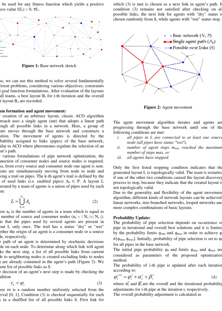
All previous researches that tackled the pipe network optimization problem with derivations of Ant Colony Optimization (ACO) method didn't really take into account all information provided by network topology. Approach presented in this paper, called Cooperative Random Walk (CRW), greatly relies on principles used in various ant-based algorithms, but it additionally utilizes the topology of a network of all possible links (base network). The base network (Figure 1) is a network of all possible pipes, from which only a subset of pipes will be used to construct possible solutions used in optimization process and, finally, the optimal network. We denote P = {i | 1 ≤ i ≤ n p} as set of all pipes in the base network, where n p is number of pipes in base network. A set N = {j | 1 ≤ j ≤ n n} represents a set of all nodes in the base network, where n n is the number of nodes. The source and consumer nodes in the base network are treated differently than other nodes in the network due to their characteristic hydraulic aspect as well as their utilization in the Cooperative Random Walk algorithm. We denote set of source nodes as Ns ⊂ N and the set of consumer nodes as Nc ⊂ N.
A specific network configuration is defined as a set of pipes used to build a layout. This set of pipes used to define a specific layout is denoted as L ⊂ P, which is effectively a representation of a design vector for the optimization process. Each (i-th) pipe in the base network at iteration t has a probability of usage which is used to direct the movement of agents explained in section A. This probability is adjusted during the optimization process, based on the obtained best solutions, as described in detail in section B. For all pipes in the base network, probability is initially set as
0
0
i
,
i
P
(1)where φ0 is the initial probability, which is a parameter of
proposed optimization method.
Like many other stochastic optimization methods, the proposed algorithm produces multiple candidates in each iteration (similar to a population in GA or a swarm in PSO). A candidate, i.e. a possible solution of the optimization problem, is discovered by a team of agents that are exploring the base network. On each iteration, n teams are used and each team is independently forming a possible solution based on the probability of links in the base network. Number of teams n is the parameter of the optimization method.
Using the team movement algorithm described in section A, in each iteration n candidate solutions are generated where each represents topologically valid solution of pipe network optimization problem. Topological validity implies that each consumer node is connected to at least one source, which automatically means there are no isolated (unconnected) pipes in network.
For each candidate a fitness function is evaluated according to the objectives and constraints of given optimization problem. Proposed method is designed as a minimization method and it
can be used for any fitness function which yields a positive fitness value f(L) > 0, ∀L.
Figure 1: Base network sketch
Thus, we can use this method to solve several fundamentally different problems, considering various objectives, constraints and goal function formulations. After evaluation of the layouts of all teams, a best layout Bt for t-th iteration and the overall
best layout Bo are recorded.
Team formation and agent movement:
For creation of an arbitrary layout, classic ACO algorithm approach uses a single agent (ant) that adopts a linear path through all possible links in a network. Here, a group of agents moves through the base network and constructs a solution. The movement of agents is directed by the probability assigned to links (pipes) of the base network, similar to ACO where pheromones regulate the selection of an agent’s path.
For various formulations of pipe network optimization, the connection of consumer nodes and source nodes is required. Thus, from every source and consumer node one agent is sent. Agents are simultaneously moving from node to node and leaving a trail on pipes. The k-th agent’s trail is defined by the list of used links (i.e. enabled pipes) Ak ⊂ P. A layout L
generated by a team of agents is a union of pipes used by each agent:
na k kA
L
1
(2)where na is the number of agents in a team which is equal to
the number of source and consumer nodes (na = | Ns |+| Nc |).
Note that the pipes used by several agents are present in layout L only once. The trail has a status "dry" or "wet" whether the origin of an agent is a consumer node or a source node, respectively.
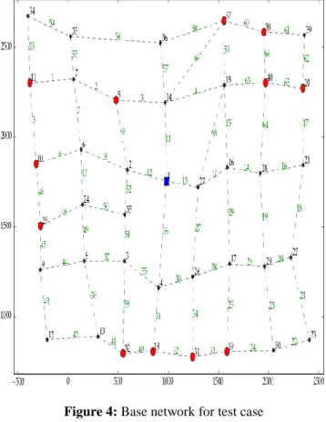
The path of an agent is determined by stochastic decisions made on each node. To determine along which link will agent make the next step, a list of all possible links from current node to neighboring nodes is created excluding links to nodes that are already contained in the agent’s path (Figure 2). We denote list of possible links as S.
The decision of an agent’s next step is made by checking the condition
i n
r
(3)where rn is a random number uniformly selected from the interval [0, 1]. Condition (3) is checked sequentially for each link in a shuffled list of all possible links S. First link for
which (3) is met is chosen as a next link in agent’s path. If condition (3) remains not satisfied after checking on all possible links, the next link for agents with "dry" status is chosen randomly from S, while agents with "wet" status stop.
Figure 2: Agent movement
The agent movement algorithm iterates and agents are progressing through the base network until one of the following conditions are met:
i. all pipes in L are connected to at least one source node (all pipes have status "wet"),
ii. number of agent steps mmax reached the maximum number of steps max, or
iii. all agents have stopped.
Only the first listed stopping condition indicates that the generated layout L is topologically valid. The team is restarted if one of the other two conditions caused the layout discovery process to stop, because they indicate that the created layout is not topologically valid.
Due to the generality and flexibility of the agent movement algorithm, different kinds of network layouts can be achieved: linear networks, tree-branched networks, looped networks and more complex combinations of basic layouts.
Probability Update:
The probability of pipe selection depends on occurrence of pipe in iterational and overall best solutions and it is limited by the probability limits min and max in order to achieve i ∊[ min, max]. Initially, probability of pipe selection is set to 0
for all pipes in the base network.
The initial pipe probability 0 and limits min and max are
considered as parameters of the proposed optimization method.
The probability of i-th pipe is updated after each iteration according to: t i t i t i t i
1
(4) where and are the overall and the iterational probability adjustments for i-th pipe at the iteration t, respectively. The overall probability adjustment is calculated as
otherwise,
)
(
if
)
(
min max 1
t i o t i t iB
i
(5)where is the overall probability adjustment factor. The adjustment α induces permanent growth of probability of pipes used in overall best layout Bo and permanent decay of
probability in other pipes of base network. We can characterize the influence of α on probability as permanent due to the fact that the overall best solution is not changing frequently. Because of a relatively unchanging αi, the
probabilities of pipes used in the overall best solution converge to a maximum value max, while for other pipes,
unused in the best layout, the probabilities decay to a minimum value min.
The iterational probability adjustment is calculated as
otherwise,
)
(
)
(
)
(
if
)
(
)
(
)
(
min 2 0 max 2 1
t i o t t i o t t iB
f
B
f
B
i
B
f
B
f
(6)where is the iterational probability adjustment factor. Since βdepends on the best solution of current iteration, it is more often changed than αand thus its influence on probability of pipe selection is instant but temporary.
Pipe Network Layout Optimization
The proposed Cooperative Random Walk algorithm described in previous section can easily be used along different objectives in pipe network optimization problems. We applied CRW to the most commonly used pipe network optimization formulation where the goal is to minimize the overall cost of the network while obeying given hydraulic constraints. Constraints for preventing incomplete or unconnected networks, which are used in other approaches, are not needed here due to the fact that CRW algorithm always produces topologically valid networks.
Hydraulic calculation:
In the research presented in this paper, EPANET 2.0 was used for the hydraulic calculations. EPANET gives an insight to the flow in each pipe and pressure at each node in the system throughout the network during a simulation period comprised of multiple time steps.
A network consists primarily of pipes and nodes. Pumps, valves, tanks or reservoirs can be added into the water distribution network. EPANET calculation is based on the laws of conservation of mass and energy in a pipe network system. These laws could also be considered as a sort of hydraulic constraints [16] that must be met.
There are three possible formulas used in EPANET for the calculation of friction head loss in a pipe. Those are the Hazen-Williams formula, which is used in this paper, the
Darcy-Weisbach formula and the Chezy-Manning formula. Using the Hazen-Williams formula components, the head loss equation is
.
727
.
4
i1.852 i4.871i i1.852 iC
D
l
Q
h
(7) where Ci stands for the Hazen-Williams roughness coefficient,which is used as Ci = 130, ∀ i, which represents cast iron as a
material for all pipes in the water distribution network. Di is
the diameter of the i-th pipe and li is the length of the i-th pipe.
A slightly different form of the Hazen-Williams equation has been introduced in [26], made particularly for optimizing water distribution networks:
i i i il
Q
C
D
h
(8)For this equation to be equivalent to the Hazen-Williams equation used in EPANET 2.0 (7), the coefficients must be equal to m = 10.6668, l = 1.852 and g = 4.871.
Fitness function:
The objective, for layout-only pipe network optimization, is to minimize the total cost of all pipes in the network. The total cost of network depends on the lengths and sizes of used pipes and, since the pipe diameter is known, it can be expressed as the sum of used pipes’ lengths in the network:
L i il
O
(9)where li is the length of the i-th pipe in layout L, and O denotes the total cost, i.e. optimization objective value. A functional pipe network layout must ensure sufficient pressure head at all consumer nodes, which can be defined as a constraint:
min
j j
p
p
,
j
N
c (10)where p and j min j
p are calculated pressure and minimal allowable pressure, respectively, for every node j in the set of consumer nodes Nc.
The minimal allowable pressure constraint (10) is not handled by the CRW algorithm directly. A penalty method is used to include handling of a constraint within a fitness function. A penalty value is defined with respect to constraint (10):
n j j j j j jp
p
p
p
p
b
a
C
1 min min minotherwise
0
if
(11)where a is the penalty jump, b is the penalty factor, and C denotes total penalty, i.e. constraint value. Finally, the fitness function, as a function of layout L, is defined as
C
O
L
f
(
)
(12)and it is used in this form to evaluate all layouts produced by the Cooperative Random Walk method. A minimization of
(12) is required to obtain the optimal layout for the described optimization problem.
A Pipe Diameter Dependent Optimal Network Layout
The Cooperative Random Walk algorithm described in the previous section is used to determine a relation between optimal pipe network layout and pipe diameter. The procedure to determine this relation is included the presented network layout optimization method, combined with the root finding algorithm. It is an iterative process (Figure 3) in which the pipe diameter is gradually decreased and optimal layout is found for each existing pipe diameter range.
For a given pipe diameter, an optimal network layout is determined by use of CRW algorithm. Using the optimal layout, a critical value of pipe diameter, for which at least one demand node has pressure equal to the minimum required pressure, is found using a simple root finding method. This can be written as finding critical diameter D crit that solves the
nonlinear equation:
(
)
0
min
min
N j crit j j cp
D
p
(13)where pressure values pj on consumer nodes Nc depend on the
pipe diameter. For solving (13) regula falsi method is used.
Figure 3: Flow diagram of algorithm for determining optimal layouts for different pipe diameters
Test
Cooperative Random Walk is better suited for layout-only optimization of pipe networks, but there is significantly more research available for simultaneous sizing and layout optimization. Results presented in [19, 21] are dealing with layout only pipe network optimization, but does not offer all information to reproduce the presented optimization cases. Thus, we designed a new test case, which is suitable for testing the proposed CRW method.
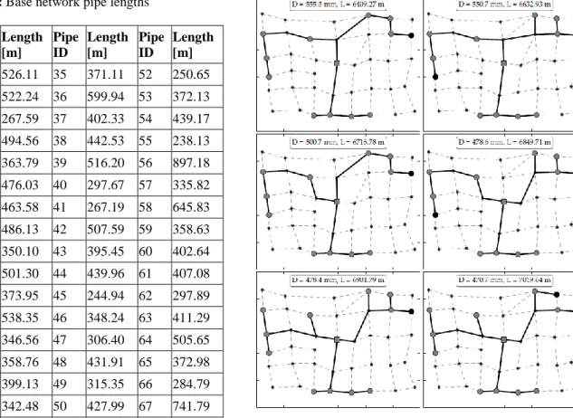
The test case is based on the base network layout shown in Figure 4. The base network is consisted of 40 nodes and 68 pipes whose lengths are given in Table 2. For simplicity, the network is considered to be ideally flat so all nodes and pipes are at the same height level. The source is located at node 1,
and it represents a reservoir with the constant water level. The head of the source node is 40 m (p 1 = 40m H20). Twelve
consumers are provided in the base network, with their outflow demand shown in Table 3. Minimal pressure needed at all consumer nodes is 10 m.
This test is designed to observe, analyze and compare optimal pipe network layouts for varying pipe diameter. There are many possible layouts which ensure that all consumer nodes are connected with the source node but not all of them satisfy the hydraulic constraints. In all this combinations, the task of this method is to find the shortest pipe network layout for a given pipe diameter that provides the consumers with the needed pressure and discharge. The main loop of the procedure gradually lowers the pipe diameter by finding the critical pipe diameter for each layout.
The pipe network layout optimization problem is different for every given pipe diameter, so it provides a completely different convergence of Cooperative Random Walk and a different final solution. Thus, the pipe diameter loop procedure is also used as a benchmark procedure for CRW method.
Figure 4: Base network for test case
Cooperative Random Walk method parameters are determined upon preliminary testing of the algorithm on various base networks. For the above described test, the optimization is done with n = 50 (number of teams) in t max = 200 iterations.
The probability adjustment = 0.035 and = 0.13 are used. Initial probability is set to 0 = 0.5 and is bounded with min = 0.03 and max = 0.90. Based on the complexity of the
base network and positions of source and consumer nodes, the maximum numbers of agent’s steps is set as m max = 4.
Table 2: Base network pipe lengths Pipe ID Length [m] Pipe ID Length [m] Pipe ID Length [m] Pipe ID Length [m] 1 437.86 18 526.11 35 371.11 52 250.65 2 440.32 19 522.24 36 599.94 53 372.13 3 489.97 20 267.59 37 402.33 54 439.17 4 598.17 21 494.56 38 442.53 55 238.13 5 455.19 22 363.79 39 516.20 56 897.18 6 452.96 23 476.03 40 297.67 57 335.82 7 400.55 24 463.58 41 267.19 58 645.83 8 477.30 25 486.13 42 507.59 59 358.63 9 405.48 26 350.10 43 395.45 60 402.64 10 312.74 27 501.30 44 439.96 61 407.08 11 437.51 28 373.95 45 244.94 62 297.89 12 394.00 29 538.35 46 348.24 63 411.29 13 316.81 30 346.56 47 306.40 64 505.65 14 329.41 31 358.76 48 431.91 65 372.98 15 460.20 32 399.13 49 315.35 66 284.79 16 430.80 33 342.48 50 427.99 67 741.79 17 428.59 34 446.06 51 258.05 68 626.14
Table 3: Consumer nodes outflow demand Node ID Outflow demand [m³/s]
5 105 10 110 11 150 18 100 19 150 20 140 25 120 31 110 32 135 37 165 38 140 40 105
The procedure for determining diameter dependent optimal pipe network layout was conducted for the described test case. To find the optimal network layout for each pipe diameter, a 100 Cooperative Random Walk optimizations are conducted and the best result is chosen as the optimal layout. Although this is a somewhat extensive computation, it gives great insurance that the optimal layout is found.
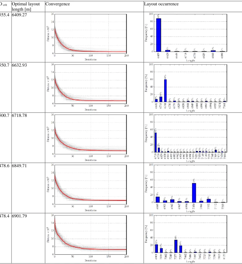
Optimal pipe network layouts are found for six different critical pipe diameters. The layouts, together with the critical
diameters and total length of the pipes in network are shown in Figure 5.
Figure 5: Optimal layouts for different pipe diameters
As expected, lowering the pipe diameter leads to longer and more complex pipe networks. Network branching is more frequent to appropriately distribute the flow which leads to lesser hydraulic losses in pipes and consequentially lower pressure in the whole network. The black circle in layouts shown in Figure 5 marks the node with the minimal pressure in the network. This is the critical node j for which p (Dj crit) =
min j
p . It is interesting to observe, when lowering the pipe diameter, additional branching occurs in the branch which contained the critical node in the previous optimal layout. Detailed illustration and comparison of the convergence of Cooperative Random Walk is displayed in Table 4. Each row of the table shows convergence information of pipe network layout optimization for given pipe diameter. The convergence plot for all 100 runs of layout optimization is shown, where average fitness value over iterations is emphasized (red line). The distribution of final fitness value, which is also the length of pipes in the network, is shown in the fourth column of the table.
Based on the convergence plots, it can be concluded that Cooperative Random Walk successfully minimizes the fitness for all six pipe diameters. Out of total 600 layout optimization runs, not a single one had a major issue with fitness minimization.
To give a more precise judgment, the distribution of final fitness value for all 100 runs should also be observed. The
proposed method is behaving differently when optimizing the same layout with different pipe diameter. The combination of pipe diameter and hydraulic constraints makes significant influence on the difficulty of the layout optimization problem which leads to premature convergence, i.e. convergence to suboptimal layout. Achievement of the optimal layout, depending on the observed pipe diameter, varies from 7% to
88%. Due to the fact that the proposed algorithm is a stochastic method where repeatability is often an issue, we believe that these results give us great confidence that Cooperative Random Walk is an appropriate and successful method for pipe network layout optimization.
Table 4: Results D crit Optimal layout
length [m]
Convergence Layout occurrence
555.4 6409.27
550.7 6632.93
500.7 6718.78
478.6 6849.71
470.7 7019.64
Conclusion
The presented technique performs full pipe network optimization coupled with pipe sizing range analysis, by employing a hydraulic model of the network and a novel heuristic optimization algorithm named Cooperative Random Walk.
Although the CRW method in principle serves as a pipe network layout optimizer, the test used for assessment of the proposed technique’s performance showed that it can be successfully used for hybrid analysis of optimal pipe diameter and network layout. The method had no problem optimizing a network of considerable size (40 nodes and 68 connections) with a satisfying success rate and repeatability.
In order to further advance the proposed pipe network optimization methodology, the pipe network cost should be made to include the full pipe cost, which is pipe-size-dependent. Even the results of the test illustrate how using smaller pipes asks for longer and more complex pipe networks in order to fulfill the demand outflow and pressure. This means that smaller pipes imply longer networks which may reduce the savings initially expected to be achieved by using smaller pipes.
Whereas the provided test network includes only one source, the CRW method itself is entirely suitable for optimizing pipe networks with many sources. Furthermore, CRW can be applied to the other pipe network optimization formulations described in the Introduction. Finally, there are other areas of network optimization where CRW should be useful, such as logistics optimization, traffic optimization, etc.
References
[1] M. Van Dijk, S. Van Vuuren, and J. Van Zyl, “Optimising water distribution systems using a weighted penalty in a genetic algorithm,” Water SA, vol. 34, no. 5, pp. 537-548, 2008.
[2] M. d. C. Cunha and J. Sousa, “Water distribution network design optimization: simulated annealing approach,” Journal of Water Resources Planning and Management, vol. 125, no. 4, pp. 215-221, 1999. [3] M. da Conceicao Cunha and L. Ribeiro, “Tabu search
algorithms for water network optimization,” European Journal of Operational Research, vol. 157, no. 3, pp. 746-758, 2004.
[4] G. C. Dandy, A. R. Simpson, and L. J. Murphy, “An improved genetic algorithm for pipe network optimization,” Water Resources Research, vol. 32, no. 2, pp. 449-458, 1996.
[5] Z. W. Geem, “Particle-swarm harmony search for water network design,” Engineering Optimization, vol. 41, no. 4, pp. 297-311, 2009.
[6] S.-Y. Liong and M. Atiquzzaman, “Optimal design of water distribution network using shuffled complex evolution,” Journal of The Institution of Engineers, Singapore, vol. 44, no. 1, pp. 93-107, 2004.
[7] H. R. Maier, A. R. Simpson, A. C. Zecchin, W. K. Foong, K. Y. Phang, H. Y. Seah, and C. L. Tan, “Ant colony optimization for design of water distribution systems,” Journal of water resources planning and management, vol. 129, no. 3, pp. 200-209, 2003. [8] M. H. Afshar, “A new transition rule for ant colony
optimization algorithms: application to pipe network optimization problems,” Engineering Optimization, vol. 37, no. 5, pp. 525-540, 2005.
[9] L. Baker and M. R.-S. Keedwell, “Ant colony optimisation for large-scale water distribution network optimisation,” in AISB 2008 Convention Communication, Interaction and Social Intelligence, vol. 1, p. 44, 2008.
[10] I. Montalvo, J. Izquierdo, R. Pérez-García, and M. Herrera, “Improved performance of pso with self-adaptive parameters for computing the optimal design of water supply systems,” Engineering applications of artificial intelligence, vol. 23, no. 5, pp. 727-735, 2010.
[11] N. Moosavian and B. K. Roodsari, “Soccer league competition algorithm: a novel meta-heuristic algorithm for optimal design of water distribution networks,” Swarm and Evolutionary Computation, vol. 17, pp. 14-24, 2014.
[12] A. Shibu and M. J. Reddy, “Cross entropy optimization for optimal design of water distribution networks,” International Journal of Computer Information Systems and Industrial Management Applications, vol. 5, pp. 308-316, 2013.
[13] M. Afshar, “Application of a max-min ant system to joint layout and size optimization of pipe networks,” Engineering optimization, vol. 38, no. 03, pp. 299-317, 2006.
[14] M. H. Afshar, “Layout and size optimization of tree-like pipe networks by incremental solution building ants,” Canadian Journal of Civil Engineering, vol. 35, no. 2, pp. 129-139, 2008.
[15] S. H. Saleh and T. T. Tanyimboh, “Coupled topology and pipe size optimization of water distribution
systems,” Water resources management, vol. 27, no. 14, pp. 4795-4814, 2013.
[16] M. H. Afshar and E. Jabbari, “Simultaneous layout and pipe size optimization of pipe networks using genetic algorithm,” Arabian Journal for Science and Engineering, vol. 33, no. 2, p. 391, 2008.
[17] R. Rajabpour and B. S. Kashkoli, “Application of discrete optimization technique hybrid jpso/lidm to optimal design of pressurized irrigation networks,” [18] R. Rajabpour and N. Talebbeydokhti, “Simultaneous
layout and pipe size optimization of pressurized irrigation networks,” Basic Research Journal of Agricultural Science and Review, vol. 3(12), pp. 131-145, 2014.
[19] A. Fugenschuh, B. Hiller, J. Humpola, T. Koch, T. Lehmann, R. Schwarz, J. Schweiger, and J. Szabo, “Gas network topology optimization for upcoming market requirements,” in Energy Market (EEM), 2011 8th International Conference on the European, pp. 346-351, IEEE, 2011.
[20] M. H. Afshar and M. A. Mariño, “Application of an ant algorithm for layout optimization of tree networks,” Engineering Optimization, vol. 38, no. 03, pp. 353-369, 2006.
[21] G. Rezaei, M. H. Afshar, and M. Rohani, “Layout optimization of looped networks by constrained ant colony optimisation algorithm,” Advances in Engineering Software, vol. 70, pp. 123-133, 2014. [22] A. Haghighi and A. E. Bakhshipour, “Optimization of
sewer networks using an adaptive genetic algorithm,” Water resources management, vol. 26, no. 12, pp. 3441-3456, 2012.
[23] Y. Setiadi, T. T. Tanyimboh, and A. Templeman, “Modelling errors, entropy and the hydraulic reliability of water distribution systems,” Advances in Engineering Software, vol. 36, no. 11, pp. 780-788, 2005.
[24] L. A. Rossman, “Epanet 2 users manual, us environmental protection agency,” Water Supply and Water Resources Division, National Risk Management Research Laboratory, Cincinnati, OH, 2000.
[25] F. Zheng, A. R. Simpson, and A. C. Zecchin, “A decomposition and multistage optimization approach applied to the optimization of water distribution systems with multiple supply sources,” Water Resources Research, vol. 49, no. 1, pp. 380-399, 2013. [26] D. A. Savic and G. A.Walters, “Genetic algorithms for least-cost design of water distribution networks,” Journal of water resources planning and management, vol. 123, no. 2, pp. 67-77, 1997.
![Table 1: Overview of pipe network optimization approaches [1] Optimization type Objective Possible variables Main constraints](https://thumb-us.123doks.com/thumbv2/123dok_us/9771832.2860658/2.892.51.451.448.959/overview-optimization-approaches-optimization-objective-possible-variables-constraints.webp)