Hybrid Approach for Detecting and Classifying Power Quality Disturbances Based on the Variational Mode Decomposition and Deep Stochastic Configuration Network

energies

Hybrid Approach for Detecting and Classifying

Power Quality Disturbances Based on the Variational

Mode Decomposition and Deep Stochastic

Configuration Network

Kewei Cai1,2 , Belema Prince Alalibo2, Wenping Cao2,* , Zheng Liu3, Zhiqiang Wang3 and Guofeng Li3

1 _{College of Information Engineering, Dalian Ocean University, Dalian 116023, China; [email protected]} 2 _{School of Engineering and Applied Science, Aston University, Birmingham, B4 7ET, UK;}

[email protected]

3 _{School of Electrical Engineering, Dalian University of Technology, Dalian 116023, China;} [email protected] (Z.L.); [email protected] (Z.W.); [email protected] (G.L.) * Correspondence: [email protected]; Tel.: +44-(0)-121-204-4264

Received: 28 September 2018; Accepted: 31 October 2018; Published: 5 November 2018

Abstract:This paper proposes a novel, two-stage and hybrid approach based on variational mode decomposition (VMD) and the deep stochastic configuration network (DSCN) for power quality (PQ) disturbances detection and classification in power systems. Firstly, a VMD technique is applied to discriminate between stationary and non-stationary PQ events. Secondly, the key parameters of VMD are determined as per different types of disturbance. Three statistical features (mean, variance, and kurtosis) are extracted from the instantaneous amplitude (IA) of the decomposed modes. The DSCN model is then developed to classify PQ disturbances based on these features. The proposed approach is validated by analytical results and actual measurements. Moreover, it is also compared with existing methods including wavelet network, fuzzy and S-transform (ST), adaptive linear neuron (ADALINE) and feedforward neural network (FFNN). Test results have proved that the proposed method is capable of providing necessary and accurate information for PQ disturbances in order to plan PQ remedy actions accordingly.

Keywords: deep stochastic configuration network (DSCN); harmonics analysis, power quality (PQ) disturbance; power system; variational mode decomposition (VMD)

1. Introduction

In power systems, power quality (PQ) has been a significant issue that is disrupted by increasing uncertain, intermittent, renewable energy penetration on the generation side [1,2] and increasing uptake of electric vehicles (EVs) on the demand side [3–5]. In essence, PQ refers to multifarious electromagnetic phenomena that deviate voltage and current from ideal waveforms, which are known as PQ disturbances (PQD). The presence of PQD can be divided into sags, swells, interruptions, oscillations, flickers, harmonics (interharmonics), notches, spikes, and their combinations, as per the international standards such as IEEE-1159, IEC 61000, and EN 50160 [6–8]. These disturbances greatly affect the safe and economical operations of power systems, decreasing the lifetime and performance of electrical equipment connected to the system. PQD analysis, including disturbances detection and classification, is an important task to provide adequate information about remedial actions to address the root problem [9–11].

In the literature, some methodologies are presented to identify the types of PQ disturbances. Signal processing methods such as Fourier transform (FT), short time Fourier transform (STFT), wavelet transform (WT), S-transform (ST), empirical mode decomposition (EMD), and independent component analysis (ICA) are extensively used to extract features for PQD detection. FT is simple to implement, but it lacks time-frequency localization capability and is unsuitable for non-stationary disturbance [12]. STFT contains both time and frequency information and can analyze non-stationary signals by sliding window [13–15]. Nevertheless, this method is limited by the sliding window size used. Although WT could enhance the time-frequency resolution for disturbance analysis [16–18], the analysis results may be affected by the noise present in the signal. The ST generalizes the STFT, extends WT and overcomes some of their disadvantages. Therefore, the ST [19] is superior compared to the FT, STFT, and WT techniques, especially for the noise-rich system. However, the computational complexity of ST limits its widespread applications. EMD is an adaptive time-frequency method for analyzing non-stationary signals and can decompose the signal into a finite number of intrinsic mode functions (IMFs) [20]. However, it will lead to false IMF decompositions due to its inherent drawbacks, e.g., mode mixing and boundary effects. To overcome these issues, an EMD-ICA technique was proposed [21]. This technique is effective at eliminating mode mixing but suffers from the absence of the amplitude information due to the added ICA. Hence, for PQ disturbance detection, it is essential to develop new signal processing techniques, which are capable of simultaneously analyzing all the nonlinear, non-stationary, and noisy signals.

As a new approach, variational mode decomposition (VMD) [22] decomposes a multimode signal into a finite number of band-limited IMFs. Compared with EMD-based methods, VMD is more robust to noise and sampling errors due to its generalization of the classic Wiener filter into multiple, adaptive bands [23,24]. Hence, for PQDs detection and classification, the disturbances feature can be extracted effectively using the VMD method; then, a classifier is used to classify different types of PQD. A noting method is proposed to combine VMD with particle swarm optimization (PSO) algorithms for fault feature extraction of rolling bearing [24]. A classification of PQ disturbances using VMD and the support vector machine (SVM) is illustrated in [25].

Other disturbance classification methods include decision tree (DT), random forest (RF), artificial neural network (ANN), probabilistic neural network (PNN), and the extreme learning machine (ELM) [26]. Among these, the SVM is the most widely used technique, which is based small sample statistics and structural risk minimization principles [27]. Similarly, DT is a decision support tool in a tree-like graph that is used to describe relationships between different features and make classifications; it has also been used to recognize PQ disturbances [28]. However, the SVM, DT, and RF methods give rise to cumulative errors in the process of the iterative classification of all disturbances. To overcome this, ANN-based classifiers have been widely used through an expeditious learning process. This process has no iterations or cumulative errors. ANN-based classifiers require a great number of training samples and often converge to local minimas [29]. PNN, derived from the Bayesian network and the kernel fisher discriminant analysis algorithm, is faster and more accurate than ANN. The existing methods are effective to enhance the performance of the classifier through complicated models, e.g., PSO and the radial basis function (RBF) kernel. Thus, the computational effort is substantially increased.

In [30], Gaing proposed a PNN-based method for classifying different types of disturbances. In order to settle previous problems, the deep stochastic configuration network (DSCN) is introduced. The DSCN [31–33] was proposed in 2017. The DSCN can assign weight and bias randomly. Hence, this technique has a faster learning speed over ANNs and better generalization capability.

The main contribution of this work lies in a novel method combining VMD and DSCN for PQ disturbances detection and classification, and VMD was used to extract PQ disturbance features. Especially, the vital parameters of VMD were discussed in detail as per different types of disturbances. Then, the features extracted were sent to DSCN for classification. The proposed method is tested by

Energies2018,11, 3040 3 of 18

seven types of synthetic PQ disturbances as well as a real time signal from the IEEE 1159.2 Working Group datasheet.

2. Variation Mode Decomposition

VMD is a non-recursive and adaptive signal processing method. It can decompose a multicomponent signal into an ensemble of band-limited IMFs, which are defined as amplitude modulated frequency modulated (AM-FM) signals with sparsity property based on Tikhonov regularization algorithm, Wiener filter, and Hilbert transformation. The IMFu(t)is illustrated as

u(t) =A(t)cos(ϕ(t)) (1)

where ϕ(t)is the phase angle, which is a nondecreasing function; the instantaneous frequency is ω(t) =ϕ0(t); andA(t)is the amplitude of the IMF. This part illustrates the structure and solution of

VMD method.

2.1. The Structure of VMD

The goal of VMD is to decompose a multicomponent signal into a finite number of sub-signals (modes),u(k), that compact around a center frequencyω(k). The process of VMD is listed as follows:

(i) Obtain the unilateral frequency spectrum of each mode by computing the associated analytic signal by means of Hilbert transform (in whichj2=−1):

δ(t) + j πt

×uk(t) (2)

(ii) Shift the frequency spectrum of each mode to baseband by multiplying an exponential tuned with estimated center frequency:

[ δ(t) + j πt ×uk(t)]e−jωkt ₍₃₎

(iii) Calculate the bandwidth of each mode by means of the squared L2-norm of the gradient. The constrained variational problem is as follows:

min{u_k},{ωk}{[ δ(t) + j πt ×uk(t)]e−jωkt_{} (4)} s.t.

∑

2.2. The Computation of VMD

A quadratic penaltyα and Lagrangian multipliersλ are introduced to address (4) to make constrained problem unconstrained. The Lagrangian operatorLis illustrated as follows [16]:

In order to solve the variational problem in (5), alternate direction method of multipliers (ADMM) is used to produce different modes and calculate the center frequencies. Each mode and center frequency obtained from solutions in spectral domain can be represented as

ˆ un_k+1(ω) = ˆ f(ω)−∑i6=kuiˆ(ω) + (λˆ(ω)/2) 1+2α(ω−ω_k)2 (6)

ω_kn+1= r∞ 0 ω|uˆk(ω)|2dω r_∞ 0 |uˆk(ω)|2dω (7) where ˆun_k+1(ω)is the result of the Wiener filter of the resident part ˆf(ω)−∑i6=kuˆi(ω);ωn_k+1is the

center frequency. Thekth modeukcan be obtained by means of an inverse Fourier Transform. Therefore, the steps of VMD algorithm can be concluded as follows:

(i) Initialize the{uˆ1_k},{ω_k1},{λˆ1}, andn=0;

(ii) Update theukandωkrepeatedly according to (6), (7); (iii) Update dual ascentλaccording to

ˆ

λn+1=λˆn+τ(fˆ(ω)−

∑

(iv) Repeat step (2), (3), until convergence:∑kkuˆnk+1−uˆnkk22/kuˆnkk22<ε.

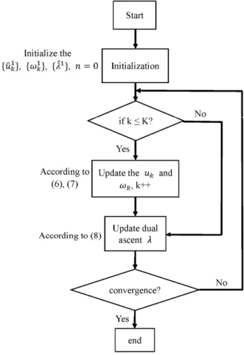
Through the above process, a finite number of IMFsukwith specific sparsity properties can be obtained non-recursively. This algorithm is more robust to noise, because wiener filter is embedded for modes update. Flow chart for solution of VMD is shown in Figure1.

Energies 2018, 11, x FOR PEER REVIEW 4 of 18

(iii) Update dual ascent 𝜆 according to

𝜆 = 𝜆 + 𝜏(𝑓(𝜔) − ∑ 𝑢 (𝜔)) (8) (iv) Repeat step (2), (3), until convergence: ∑ ‖𝑢 − 𝑢 ‖ /‖𝑢 ‖ < 𝜀.

Through the above process, a finite number of IMFs 𝑢 with specific sparsity properties can be obtained non-recursively. This algorithm is more robust to noise, because wiener filter is embedded for modes update. Flow chart for solution of VMD is shown in Figure 1.

Figure 1. Flow chart of the variational mode decomposition (VMD). 2.3. Determination of VMD Parameters

There are three key parameters impacting the alluring of the feature methods, namely, Lagrangian multiplier λ, number of modes K, and regularization factor 𝛼.

(i) Lagrangian Multiplier λ

The Lagrangian multiplier is selected to enforce the equality constraint of reconstruction. It can be set to zero if exact reconstruction is not required, particularly in noisy conditions. In this work, it is done by simply choosing its update parameter τ = 0 in term (8).

(ii) Number of Modes K

K denotes the number of modes from the VMD analysis results. If it is small, the result suffers from mode mixing, there multiple modes are present in one mode component. If it is large, the result suffers from mode redundancy, where a mode is decomposed into many modes components. In this paper, K is determined based on the number of voltage peaks in frequency domain from FFT results.

Figure 1.Flow chart of the variational mode decomposition (VMD).

2.3. Determination of VMD Parameters

There are three key parameters impacting the alluring of the feature methods, namely, Lagrangian multiplierλ, number of modesK, and regularization factorα.

Energies2018,11, 3040 5 of 18

The Lagrangian multiplier is selected to enforce the equality constraint of reconstruction. It can be set to zero if exact reconstruction is not required, particularly in noisy conditions. In this work, it is done by simply choosing its update parameterτ= 0 in term (8).

(ii) Number of ModesK

Kdenotes the number of modes from the VMD analysis results. If it is small, the result suffers from mode mixing, there multiple modes are present in one mode component. If it is large, the result suffers from mode redundancy, where a mode is decomposed into many modes components. In this paper,Kis determined based on the number of voltage peaks in frequency domain from FFT results.

(iii) Regularization factorα

The term (5) is the classical Tikhonov regularization problem whenλ=0, in which the penalty

parameterαis actually regularization factor. Whenαis small, the constraint termkf(t)−∑K_k=1uk(t)k2₂

can be easily satisfied, whereas the penalty term k∂t h δ(t) + _πj_t ×uk(t) i e−jωktk2

2 does not have adequate penalty; we can not expect the mode and center frequency to be detected precisely. Whenα

is large, the constraint termkf(t)−_∑K

k=1uk(t)k22could not to be satisfied; we expect that the center frequenciesωkand corresponding IMFsuk(t)might be estimated precisely under noisy and noise-free environments. However, the center frequencies would converge to the same frequency to lead mode redundant and missed due to the local optimization property of VMD [16]. Hence, value ofαcan

be kept low (of the range of few hundreds) in order to capture signals containing wide range of frequencies, while for detection of frequency components of signal over smaller range, it should be kept larger (in the range of tens of thousands). In this paper, we selectedαaccording to different

disturbances analysis condition combining parameter K andωk, as shown in following section. 2.4. PQ Disturbances Analysis

In order to demonstrate the effectiveness of VMD for harmonic signal decomposition, a synthetic signal was established in MATLAB, which is given by:

v(t) =

∑

where Am, fm, ψm, and n(t) are the amplitude, frequency, phase angle of different components,

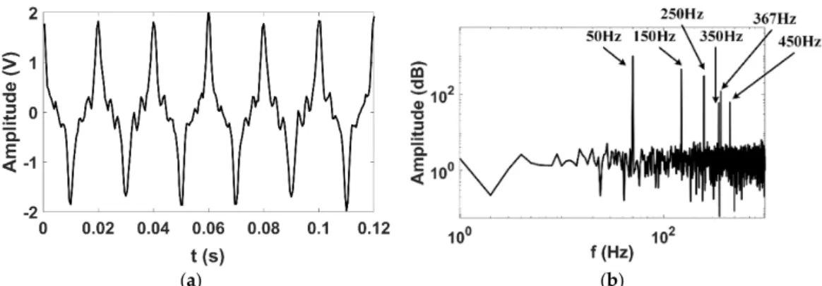
and white noise respectively. The waveform is sampled at 2 kHz. The number of samples is 2000, and the resolution of this signal is 1 Hz. The synthetic signal is composed of a fundamental component, four harmonic components, one interharmonic component and white noise. The magnitude and frequency spectrum of the synthetic voltage are shown in Figure2.

Energies 2018, 11, x FOR PEER REVIEW 5 of 18

(iii) Regularization factor 𝛼

The term (5) is the classical Tikhonov regularization problem when 𝜆 = 0, in which the penalty parameter 𝛼 is actually regularization factor. When 𝛼 is small, the constraint term ‖𝑓(𝑡) − ∑ 𝑢 (𝑡)‖ can be easily satisfied, whereas the penalty term ∂ 𝛿(𝑡) + × 𝑢 (𝑡) 𝑒 does not have adequate penalty; we can not expect the mode and center frequency to be detected precisely. When 𝛼 is large, the constraint term ‖𝑓(𝑡) − ∑ 𝑢 (𝑡)‖ could not to be satisfied; we expect that the center frequencies 𝜔 and corresponding IMFs 𝑢 (𝑡) might be estimated precisely under noisy and noise-free environments. However, the center frequencies would converge to the same frequency to lead mode redundant and missed due to the local optimization property of VMD [16]. Hence, value of 𝛼 can be kept low (of the range of few hundreds) in order to capture signals containing wide range of frequencies, while for detection of frequency components of signal over smaller range, it should be kept larger (in the range of tens of thousands). In this paper, we selected 𝛼 according to different disturbances analysis condition combining parameter K and 𝜔 , as shown in following section.

2.4. PQ Disturbances Analysis

In order to demonstrate the effectiveness of VMD for harmonic signal decomposition, a synthetic signal was established in MATLAB, which is given by:

𝑣(𝑡) = ∑ 𝐴 cos(2𝜋𝑓 𝑡 + 𝜓 ) + 0.05𝑛(𝑡) (9) where 𝐴 , 𝑓 , 𝜓 , and 𝑛(𝑡) are the amplitude, frequency, phase angle of different components, and white noise respectively. The waveform is sampled at 2 kHz. The number of samples is 2000, and the resolution of this signal is 1 Hz. The synthetic signal is composed of a fundamental component, four harmonic components, one interharmonic component and white noise. The magnitude and frequency spectrum of the synthetic voltage are shown in Figure 2.

(a) (b)

Figure 2. The magnitude and frequency spectrum of the grid voltage, (a) magnitude, and (b) frequency spectrum.

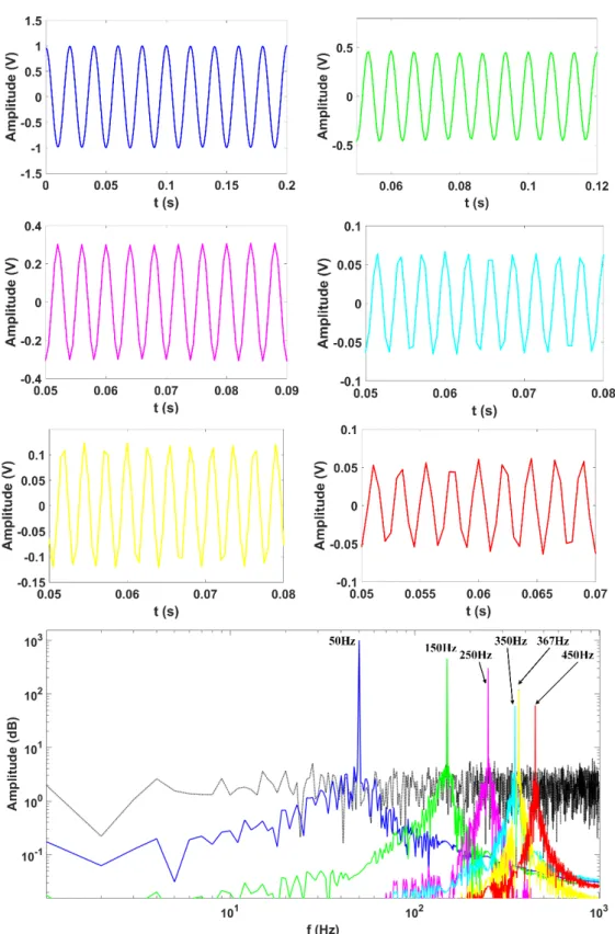
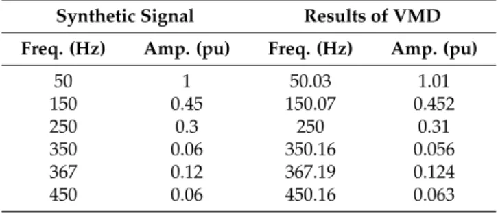
Next, we used VMD to separate the synthetic signal. Considering both precise requirement and noisy level of voltage signal, we chose K = 6, according to wave packages of frequency spectrum of waveform, 𝛼 = 20,000 and 𝜔 = 50, 150, 250, 350, 367, and 450 Hz, respectively, in order to avoid the adverse effect of local optimum property of VMD, in which the interharmonics frequency is 367 Hz and harmonics frequencies are 150, 250, 350, and 450 Hz, respectively. The decomposed modes and their frequency spectrum are illustrated in Table 1 and Figure 3.

Figure 2. The magnitude and frequency spectrum of the grid voltage: (a) magnitude, and (b) frequency spectrum.

Next, we used VMD to separate the synthetic signal. Considering both precise requirement and noisy level of voltage signal, we chose K = 6, according to wave packages of frequency spectrum of waveform,α=20, 000 andωini =50, 150, 250, 350, 367, and 450 Hz, respectively, in order to avoid

the adverse effect of local optimum property of VMD, in which the interharmonics frequency is 367 Hz and harmonics frequencies are 150, 250, 350, and 450 Hz, respectively. The decomposed modes and their frequency spectrum are illustrated in TableEnergies 2018, 11, x FOR PEER REVIEW 1and Figure3. 6 of 18

Figure 3. The decomposed modes and their frequency spectrum.

As can be seen in Figure 3, the spectrum of all frequencies was decomposed distinctly and had high degree of correlation with the theoretical modes. The modes of the signal that were recovered by VMD constitute a good partition of the original signal spectrum. In Figure 3 and Table 1, each mode was clearly dominant around its respective center frequency. Almost all components were

Figure 3.The decomposed modes and their frequency spectrum.

As can be seen in Figure3, the spectrum of all frequencies was decomposed distinctly and had high degree of correlation with the theoretical modes. The modes of the signal that were recovered by VMD constitute a good partition of the original signal spectrum. In Figure3and Table1, each mode

Energies2018,11, 3040 7 of 18

was clearly dominant around its respective center frequency. Almost all components were extracted flawlessly, except the fifth and seventh order ones. This is due to the fact that the amplitudes of these two modes are both close to noise. The Signal-to-Noise-Ratio (SNR) is only−1.49 dB.

Table 1.Results of variational mode decomposition (VMD) for harmonics and interharmonics extraction.

Synthetic Signal Results of VMD Freq. (Hz) Amp. (pu) Freq. (Hz) Amp. (pu)

50 1 50.03 1.01 150 0.45 150.07 0.452 250 0.3 250 0.31 350 0.06 350.16 0.056 367 0.12 367.19 0.124 450 0.06 450.16 0.063 2.5. Flicker Separation

Flicker waveform, which has amplitude envelope with low frequency component, was modelled mathematically as in Formula (10)

v(t) =A0+

∑

cos(2πf0t+ϕ0) (10) According to trigonometric identities, we could expand term (10) to (11)

v(t) = A0cos(2πf0t+ϕ0) +12∑nAn{cos(2π(f0+fn)t+ (ϕ0+ϕn)) +cos(2π(f0−fn)t+ (ϕ0−ϕn))} (11)

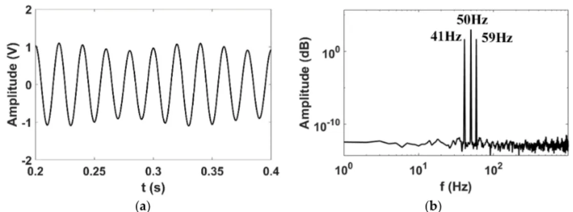
Hence, as shown in Formula (11), each flicker with frequencyfn(< f0)is decomposed into two components with frequency f0±fn. In nature, voltage signal with flicker component is composed of fundamental component (f0) and two other (f0±fn) components, whose frequency is close tof0. In this paper, we assume that f0 =50 Hz, fn = 9 Hz,A0 =1(pu), andAn = 0.1(pu). In order to separate flicker precisely using VMD, we chose large regularization factorα = 20, 000;K= 3; and initialize ωini=41, 50, 59 Hz, respectively.

The magnitude and frequency spectrum of it is shown in Figure4. The decomposed modes and their frequency spectrum are illustrated in Table2and Figure5.

From above results, the effectiveness of VMD technique has been evaluated. This method could capture the flicker components accurately as well as fundamental voltage. Since the flicker frequency is 9 Hz, spectrum of decomposed modes showed 41 (50–9) Hz with 0.049 amplitude in pu and 59 (50 + 9) Hz with 0.05 amplitude in pu. The sum of amplitude, which is 0.099, was in high accordance with flicker component of the synthetic voltage.

Table 2.Results of VMD for flicker extraction.

Parameter Synthetic Signal Results of VMD

A0(pu) 1 0.999

f0(Hz) 50 50.03

An(pu) 0.4 0.049 + 0.05 = 0.099

f0−fn(Hz) 41 41.02

Energies 2018, 11, x FOR PEER REVIEW 8 of 18

(a) (b)

Figure 4. The magnitude and frequency spectrum of the grid voltage, (a) magnitude, and (b) frequency spectrum.

Figure 5. The decomposed modes and their frequency spectrum.

3. Power Disturbance Detection and Classification based on VMD and DSCN

The DSCN technique is a novel artificial algorithm and is used as a classifier to identify power disturbances.

3.1. Deep Stochastic Configuration Networks Algorithm

In the past decade, DNNs have received considerable attention and become increasingly popular due to the hypothesis that a deep network model can be more effective in data representation than shallow ones [31,33]. DSCN is developed based on stochastic configuration network (SCN), which is proposed in [33].

A typical DSCN architecture is illustrated in Figure 6, in which number of hidden layers and first hidden layer nodes are n = 2, 𝐿 = 3; the second hidden layer nodes satisfy 𝐿 = 2, with 2 input nodes and one output node as well.

A target function can be defined as Ƒ: 𝑅 → 𝑅 , with n hidden layers and L (𝑘 = 1,2, … , 𝑛) hidden nodes in each layer, that is,

Figure 4. The magnitude and frequency spectrum of the grid voltage: (a) magnitude, and (b) frequency spectrum.

Energies 2018, 11, x FOR PEER REVIEW 8 of 18

(a) (b)

Figure 4. The magnitude and frequency spectrum of the grid voltage, (a) magnitude, and (b) frequency spectrum.

Figure 5. The decomposed modes and their frequency spectrum.

3. Power Disturbance Detection and Classification based on VMD and DSCN

The DSCN technique is a novel artificial algorithm and is used as a classifier to identify power disturbances.

3.1. Deep Stochastic Configuration Networks Algorithm

In the past decade, DNNs have received considerable attention and become increasingly popular due to the hypothesis that a deep network model can be more effective in data representation than shallow ones [31,33]. DSCN is developed based on stochastic configuration network (SCN), which is proposed in [33].

A typical DSCN architecture is illustrated in Figure 6, in which number of hidden layers and first hidden layer nodes are n = 2, 𝐿 = 3; the second hidden layer nodes satisfy 𝐿 = 2, with 2 input nodes and one output node as well.

A target function can be defined as Ƒ: 𝑅 → 𝑅 , with n hidden layers and L (𝑘 = 1,2, … , 𝑛) hidden nodes in each layer, that is,

Figure 5.The decomposed modes and their frequency spectrum.

3. Power Disturbance Detection and Classification based on VMD and DSCN

The DSCN technique is a novel artificial algorithm and is used as a classifier to identify power disturbances.

3.1. Deep Stochastic Configuration Networks Algorithm

In the past decade, DNNs have received considerable attention and become increasingly popular due to the hypothesis that a deep network model can be more effective in data representation than shallow ones [31,33]. DSCN is developed based on stochastic configuration network (SCN), which is proposed in [33].

A typical DSCN architecture is illustrated in Figure6, in which number of hidden layers and first hidden layer nodes aren= 2,L1=3; the second hidden layer nodes satisfyL2=2, with 2 input nodes and one output node as well.

A target function can be defined asF : Rd→Rm, with n hidden layers and Lk(k=1, 2, . . . ,n) hidden nodes in each layer, that is,

F_L(n) n (x) =

∑

∑

Energies2018,11, 3040 9 of 18

in whichw(_jk−1),b(_jk−1)are the hidden parameters within the kth hidden layer, ϕk,j stands for the activation function inkth hidden layer,x(k)=

ϕk,1,ϕk,2, . . . ,ϕk,Lk

andx(0)_{=xare for initialization,}

and the residual error function is defined byε(_Ln)

n =F − F (n)

Ln .

The method starts with a small sized network (e.g., one hidden layer with one hidden node) and stochastically configures its nodes for the current layer until a certain termination criterion is met; then, it continues to add the next hidden layer by repeating the same procedures and keeps proceeding to deeper layers until an acceptable error tolerance has been achieved. As the constructive process proceeds, the hidden parameters are randomly assigned under a supervisory mechanism, while the read-out weights linking the hidden nodes to the output nodes are calculated by the least squares method [32]. Thus, the DSCN algorithm decides the number of hidden layers and nodes dynamics as per the training data, which has addressed the design and fast implementation problems of DNNs.

Energies 2018, 11, x FOR PEER REVIEW 9 of 18

Ƒ( )(𝑥) = ∑ ∑ 𝛽( )φ ,(𝑥( ); 𝑤( ), 𝑏( )) (12)

in which 𝑤( ), 𝑏( ) are the hidden parameters within the kth hidden layer, 𝜑, stands for the activation function in kth hidden layer, 𝑥( )= [𝜑, , 𝜑 , , … , 𝜑, ] and 𝑥( )= 𝑥 are for initialization, and the residual error function is defined by Ɛ( )= Ƒ − Ƒ( ).

The method starts with a small sized network (e.g., one hidden layer with one hidden node) and stochastically configures its nodes for the current layer until a certain termination criterion is met; then, it continues to add the next hidden layer by repeating the same procedures and keeps proceeding to deeper layers until an acceptable error tolerance has been achieved. As the constructive process proceeds, the hidden parameters are randomly assigned under a supervisory mechanism, while the read-out weights linking the hidden nodes to the output nodes are calculated by the least squares method [32]. Thus, the DSCN algorithm decides the number of hidden layers and nodes dynamics as per the training data, which has addressed the design and fast implementation problems of DNNs.

Figure 6. Typical deep stochastic configuration network (DSCN) diagram.

3.2. Disturbance Detection and Classification

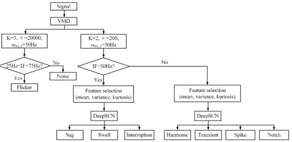
In this section, we proposed a two-stage detection and classification method for PQ disturbance identification. The structure of this theory is illustrated in Figure 7.

Figure 7. The flowchart of the proposed power quality disturbance (PQD) detection and classification method.

Figure 6.Typical deep stochastic configuration network (DSCN) diagram.

3.2. Disturbance Detection and Classification

In this section, we proposed a two-stage detection and classification method for PQ disturbance identification. The structure of this theory is illustrated in Figure7.

Energies 2018, 11, x FOR PEER REVIEW 9 of 18

Ƒ( )(𝑥) = ∑ ∑ 𝛽( )φ,(𝑥( ); 𝑤( ), 𝑏( )) (12) in which 𝑤( ), 𝑏( ) are the hidden parameters within the kth hidden layer, 𝜑 , stands for the activation function in kth hidden layer, 𝑥( )= [𝜑 , , 𝜑 , , … , 𝜑 , ] and 𝑥( )= 𝑥 are for initialization, and the residual error function is defined by Ɛ( )= Ƒ − Ƒ( ).

The method starts with a small sized network (e.g., one hidden layer with one hidden node) and stochastically configures its nodes for the current layer until a certain termination criterion is met; then, it continues to add the next hidden layer by repeating the same procedures and keeps proceeding to deeper layers until an acceptable error tolerance has been achieved. As the constructive process proceeds, the hidden parameters are randomly assigned under a supervisory mechanism, while the read-out weights linking the hidden nodes to the output nodes are calculated by the least squares method [32]. Thus, the DSCN algorithm decides the number of hidden layers and nodes dynamics as per the training data, which has addressed the design and fast implementation problems of DNNs.

Figure 6. Typical deep stochastic configuration network (DSCN) diagram. 3.2. Disturbance Detection and Classification

In this section, we proposed a two-stage detection and classification method for PQ disturbance identification. The structure of this theory is illustrated in Figure 7.

Figure 7. The flowchart of the proposed power quality disturbance (PQD) detection and classification method.

Figure 7. The flowchart of the proposed power quality disturbance (PQD) detection and classification method.

Firstly, the proposed method decomposed flicker and other disturbances with different parameters of VMD. A large value of regularization factorα(α= 20,000), number of modesK(K= 3), and initial

instantaneous frequency (IF) of modes was used to assess if flicker is existed as per IEEE Std. 1159–2009 [8]. Then, for the other power disturbances, another group of parameters of VMD was applied to decompose stationary and non-stationary types of disturbances. The fundamental component that contains stationary disturbance like sag, swell, and interruption is separated using K = 2 and ωini_1 = 50 Hz, while the non-stationary disturbances, e.g., harmonic, transient, spike, and notch, were all included in the remaining component. A small value of regularization factorα

(α= 200) is chosen to retain multi-frequency modes of non-stationary disturbance. Afterwards, several

types of statistical information (mean, variance, and kurtosis) are extracted from instantaneous amplitude (IA) of decomposed modes as disturbance features. Finally, the DSCN method is applied to classify stationary and non-stationary disturbances by means of mean, variance, and kurtosis. 4. Results and Discussion

In order to validate the proposed method, both synthetic and real-world PQ disturbance signals were acquired and used for constructing analytical models.

4.1. Synthetic Signal

Based on synthetic signals, four types of mixed PQ disturbances are established: (1) interruption with oscillation, (2) sag with harmonics, (3) swell with notch, and (4) swell with spike. The synthetic models are then constructed in MATLAB. There are 200 sample signals to establish for each disturbance, where 150 are for training model and 50 for testing. Each synthetic signal is sampled at 2 kHz. The number of samples is 2000, and the resolution of this signal is 1 Hz.

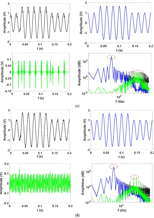
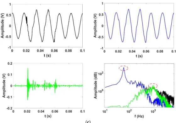
In the first stage, the PQ disturbance signal is composed of fundamental and transient components withK= 2,α= 200, andωini_1= 50 Hz. The results are illustrated in Figure8.

The fundamental component was fully decomposed in first mode (circle flagged in spectrum), which concluded all stationary disturbances, e.g., interruption, sag, and swell, while impulse component, which included non-stationary disturbances, e.g., oscillation, harmonics, notch, and spike, was separately extracted in the second mode. In the first stage, stationary and non-stationary disturbances were separated into two parts. Then, three statistics features, which are mean, variance, and kurtosis, were extracted to define a feature matrix of DSCN for classification in the second stage of proposed method.

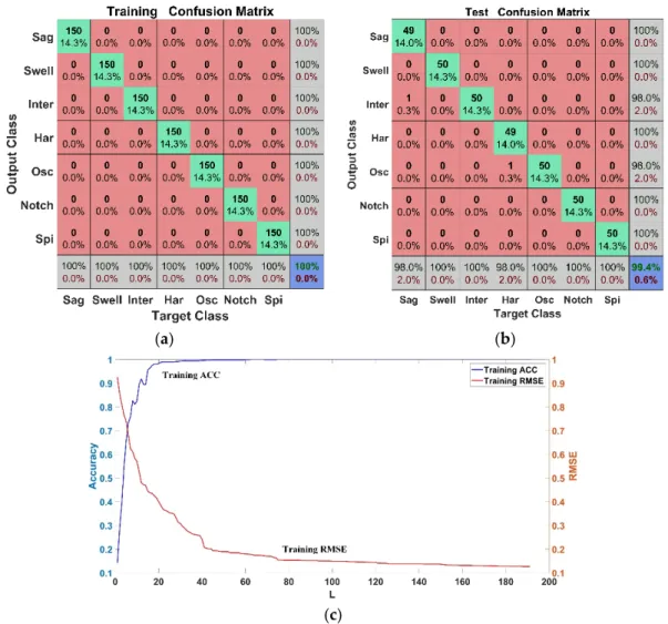
More specifically, the weights and biases of DSCN are randomly assigned under a supervisory mechanism, while the number of layers and nodes in each hidden layer is contributed automatically according to a specific termination criterion. DSCN starts with a small network and stochastically configures its nodes for the current layer until the termination criterion is met. Then, a hidden layer is added by the DSCN proceeds until an acceptable error tolerance is achieved. In the proposed method, a supervisory range is set to a parameter, and actual parameters are randomly assigned by the DSCN. For instance, the maximum node number in a hidden layer (Lmax) is set at 200, and the range of weights and biases (λ) is 0.5 to 100. The termination criterion (tol) is 0.01. Under this condition, DSCN produced 3 hidden layers, 191 nodes in each layer, 3×191 stochastic weight values, and 1×191 stochastic bias values in our work. The classification rates are 100% and 99.4% in the training and the test fusion matrices, respectively. The results of classification are shown in Figure9.

Energies2018,11, 3040 11 of 18

Energies 2018, 11, x FOR PEER REVIEW 11 of 18

(a)

(b)

Energies 2018, 11, x FOR PEER REVIEW 12 of 18

(c)

(d)

Figure 8. The decomposed voltage results using VMD: (a) interruption with oscillation, (b) sag with harmonics, (c) swell and notch, and (d) swell with spike.

Figure 8.The decomposed voltage results using VMD: (a) interruption with oscillation, (b) sag with harmonics, (c) swell and notch, and (d) swell with spike.

Energies2018,11, 3040 13 of 18

Energies 2018, 11, x FOR PEER REVIEW 13 of 18

(a) (b)

(c)

Figure 9. The results of classification: (a) training confusion matrix, (b) test confusion matrix, and (c) accuracy and root mean square error (RMSE) curve of training.

4.2. Real World Signal

Following the synthetic signals, a real-world PQ disturbance signal from the IEEE 1159.2 Working Group datasheet is used for validating the proposed method. The signal under test is based on the three-phase voltages which are contaminated for sag, swell, and oscillatory transient events. The signals were all analyzed using the proposed method with parameters being K = 2, α = 200, and

ωini_1 = 50 Hz. The results are shown in Figure 10.

It can be observed from Figure 8 that the fundamental component was fully decomposed in the first mode (circle flagged in spectrum), which concluded all stationary disturbances, sag (in phase A), and swell (in phase B and C), while impulse component (square flagged in spectrum), which included oscillatory transient events, was separately extracted in the second mode.

4.3. Discussion

In synthetic signals, as can be seen from Figure 9, the classification rate in the training matrix was 100% for all disturbances. The number of the simulated events was 150 for training the model. As shown in Figure 7c, the training accuracy was higher than 0.99 when 40 nodes were established in the hidden layer; moreover, the training RMSE was lower than 0.18. While 50 events were used for testing, the total classification rate was 99.4%, as shown in Figure 7b. Results demonstrated that the proposed method based on the VMD and DSCN can achieve an excellent detection and classification rates for disturbances. Additionally, the results of proposed method were compared to other techniques in Tables 3 and 4.

Figure 9.The results of classification: (a) training confusion matrix, (b) test confusion matrix, and (c) accuracy and root mean square error (RMSE) curve of training.

4.2. Real World Signal

Following the synthetic signals, a real-world PQ disturbance signal from the IEEE 1159.2 Working Group datasheet is used for validating the proposed method. The signal under test is based on the three-phase voltages which are contaminated for sag, swell, and oscillatory transient events. The signals were all analyzed using the proposed method with parameters being K= 2, α= 200,

andωini_1= 50 Hz. The results are shown in Figure10.

It can be observed from Figure8that the fundamental component was fully decomposed in the first mode (circle flagged in spectrum), which concluded all stationary disturbances, sag (in phase A), and swell (in phase B and C), while impulse component (square flagged in spectrum), which included oscillatory transient events, was separately extracted in the second mode.

4.3. Discussion

In synthetic signals, as can be seen from Figure9, the classification rate in the training matrix was 100% for all disturbances. The number of the simulated events was 150 for training the model. As shown in Figure7c, the training accuracy was higher than 0.99 when 40 nodes were established in the hidden layer; moreover, the training RMSE was lower than 0.18. While 50 events were used for testing, the total classification rate was 99.4%, as shown in Figure7b. Results demonstrated that the proposed method based on the VMD and DSCN can achieve an excellent detection and classification rates for

disturbances. Additionally, the results of proposed method were compared to other techniques in TablesEnergies 32018and, 114, x FOR PEER REVIEW . 14 of 18

(a)

(b)

Energies2018,11, 3040 15 of 18

Energies 2018, 11, x FOR PEER REVIEW 15 of 18

(c)

Figure 10. The decomposed results of four real-time signals by using VMD, (a) phase A, (b) phase B, and (c) phase C.

The accuracy comparison of the proposed PQ assessment framework with other methods was illustrated in Table 3 with four methods including EMD and balanced neural tree [20], ST and NN with DT [34], Hybrid ST and DT [35], and ADALINE and FNN [29]. The evaluation results showed that the proposed framework has comparatively better performance over most of other existing methods. The accuracy of ST combined with NN and DT methods proposed in [34] was slightly higher than the proposed method.

From the above analysis, the proposed method is excellent in the following aspects. Firstly, the developed VMD is capable of detecting PQD as a feature extraction method. The key parameters of VMD are determined as per different types of disturbance. Secondly, three statistical features (mean, variance, and kurtosis) are extracted from instantaneous amplitude of the decomposed modes. Finally, different types of disturbance are classified by the DSCN, which has a faster learning speed and better generalization capability than existing methods.

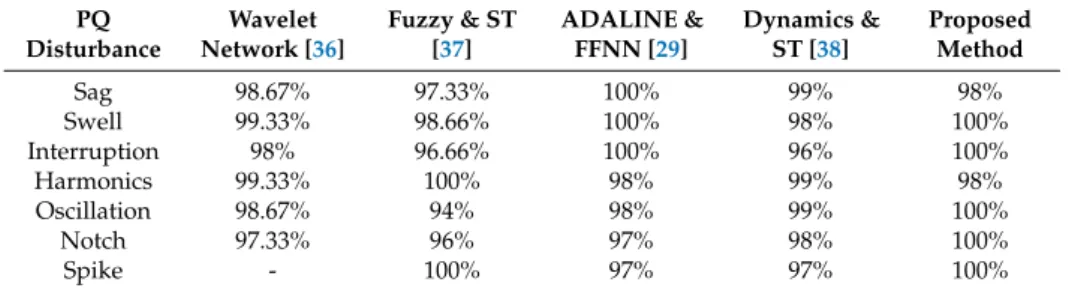
However, the NN and DT algorithms are combined for classification [27], which complicates the classified process and increases its computing time. While DSCN method is used as a classifier in the proposed method, the accuracy is similar. The tradeoff between the accuracy and complexity is typical, subject to their computational costs. Additionally, the accuracy comparison for specific event of the proposed method with other techniques was illustrated in Table 4 with four methods including wavelet network [36], fuzzy and ST [37], ADALINE and FNN [29], and dynamics and ST [38]. It was observed that the proposed method showed better classification capability, since the VMD approach in the first stage of this method had separated the stationary and non-stationary disturbances effectively, which simplified the classification process in DSCN in the second stage of the method. It can be seen from Figure 10 that the proposed method can also locate the moment when disturbances occur and is capable of capturing the start and finish of the disturbance.

Figure 10.The decomposed results of four real-time signals by using VMD: (a) phase A, (b) phase B, and (c) phase C.

The accuracy comparison of the proposed PQ assessment framework with other methods was illustrated in Table3with four methods including EMD and balanced neural tree [20], ST and NN with DT [34], Hybrid ST and DT [35], and ADALINE and FNN [29]. The evaluation results showed that the proposed framework has comparatively better performance over most of other existing methods. The accuracy of ST combined with NN and DT methods proposed in [34] was slightly higher than the proposed method.

From the above analysis, the proposed method is excellent in the following aspects. Firstly, the developed VMD is capable of detecting PQD as a feature extraction method. The key parameters of VMD are determined as per different types of disturbance. Secondly, three statistical features (mean, variance, and kurtosis) are extracted from instantaneous amplitude of the decomposed modes. Finally, different types of disturbance are classified by the DSCN, which has a faster learning speed and better generalization capability than existing methods.

However, the NN and DT algorithms are combined for classification [27], which complicates the classified process and increases its computing time. While DSCN method is used as a classifier in the proposed method, the accuracy is similar. The tradeoff between the accuracy and complexity is typical, subject to their computational costs. Additionally, the accuracy comparison for specific event of the proposed method with other techniques was illustrated in Table4with four methods including wavelet network [36], fuzzy and ST [37], ADALINE and FNN [29], and dynamics and ST [38]. It was observed that the proposed method showed better classification capability, since the VMD approach in the first stage of this method had separated the stationary and non-stationary disturbances effectively, which simplified the classification process in DSCN in the second stage of the method. It can be seen from Figure10that the proposed method can also locate the moment when disturbances occur and is capable of capturing the start and finish of the disturbance.

Table 3.The accuracy comparison of the proposed PQ assessment framework with other methods.

Feature Extraction Method Type of Classifier No. of PQ

Disturbance Accuracy (%) Ref.

EMD Balanced Neural Tree 8 97.9 [20]

ST NN+DT 13 99.9 [34]

Hybrid ST DT 11 94.36 [35]

ADALINE FNN 12 90.58 [29]

VMD DSCN 7 99.4 Proposed method

Table 4.The accuracy comparison of specific events of the proposed method and other techniques.

PQ Disturbance Wavelet Network [36] Fuzzy & ST [37] ADALINE & FFNN [29] Dynamics & ST [38] Proposed Method Sag 98.67% 97.33% 100% 99% 98% Swell 99.33% 98.66% 100% 98% 100% Interruption 98% 96.66% 100% 96% 100% Harmonics 99.33% 100% 98% 99% 98% Oscillation 98.67% 94% 98% 99% 100% Notch 97.33% 96% 97% 98% 100% Spike - 100% 97% 97% 100% 5. Conclusions

In this paper, a new algorithm based on VMD and DSCN is developed for the detection and classification of PQ disturbances. In the detection stage, the VMD can deal with the time and frequency resolutions of stationary and non-stationary PQ events. The key parameters in the VMD method are determined as per the disturbances. All the PQ events can also be located precisely by means of VMD. This algorithm is excellent in feature extraction. In terms of classification, the DSCN has a faster learning speed and better generalization capability than existing methods. It does not need complicated models to optimize the classifier, while existing methods do. Thus, the computational effort is substantially decreased compared to the existing algorithms. Finally, a real-world PQ event and simulated events are used to confirm the effectiveness of the proposed method.

However, the proposed method has been tested through offline analysis. In the future work, it will be implemented online in hardware in the loop system. The computational speed of the VMD and DSCN methods needs to be improved in this respect.

Author Contributions:Conceptualization, K.C. and W.C.; methodology, W.C.; validation, K.C.; formal analysis, B.P.A.; investigation, B.P.A.; data curation, B.P.A. and G.L.; writing—original draft preparation, K.C.; writing—review and editing, K.C., W.C., Z.L., and Z.W.; visualization, K.C.; supervision, W.C. and G.L.; project administration, K.C.; funding acquisition, K.C. and W.C.

Funding: This research was funded by the Foundation of Liaoning Province Education Administration (grant number L201609), the Doctoral Start-up Foundation of Liaoning Province (grant number 20170520191) and the Royal Society U.K.

Conflicts of Interest:The authors declare there is no conflicts of interest regarding the publication of this paper.

References

1. Díaz-Araujo, M.; Medina, A.; Cisneros-Magaña, R.; Ramírez, A. Periodic steady state assessment of microgrids with photovoltaic generation using limit cycle extrapolation and cubic splines.Energies2018, 11, 2096. [CrossRef]

2. Deng, C.H.; Chen, Y.H.; Tan, J.; Xia, P.; Liang, N.; Yao, W.W.; Zhang, Y.A. Distributed variable droop curve control strategies in smart microgrid.Energies2017,11, 24. [CrossRef]

3. González-De-La-Rosa, J.J.; Agüera-Pérez, A.; Palomares-Salas, J.C.; Florencias-Oliveros, O.; Sierra-Fernández, J.M. A dual monitoring technique to detect power quality transients based on the fourth-order spectrogram.

Energies2018,11, 3040 17 of 18

4. Rosa, J.J.G.; Sierra-Fernández, J.M.; Agüera-Pérez, A.; Palomares-Salas, J.C.; Moreno-Muñoz, A. An application of the spectral kurtosis to characterize power quality events.Int. J. Electr. Power Energy Syst.2015,49, 386–398. [CrossRef]

5. Lucas, A.; Trentadue, G.; Scholz, H.; Otura, M. Power quality performance of fast-charging under extreme temperature conditions.Energies2018,11, 2635. [CrossRef]

6. Voltage Characteristics of Electricity Supplied by Public Distribution Systems; Belgian Standards: Belgium, 1994.

7. Testing and Measurement Techniques Power Quality Measurement Methods; IEC 61000-4-30; International

Electrotechnical Commission: Geneva, Switzerland, 2003.

8. IEEE Recommended Practice for Monitoring Electric Power Quality; IEEE Standard 1159–2009; IEEE: Piscataway,

NI, USA, 2009.

9. Javadi, A.; Al-Haddad, K. A single phase active device for power quality improvement of electric field transportation.IEEE Trans. Ind. Electron.2015,62, 3033–3041. [CrossRef]

10. Xiao, H.; Wei, J.; Li, Q. Identification of combined power quality disturbances using singular value decomposition (SVD) and Total Least Squares-Estimation of Signal Parameters via Rotational Invariance Techniques (TLS-ESPRIT).Energies2017,10, 1809. [CrossRef]

11. Pérez-Ortiz, M.; Jiménez-Fernández, S.; Gutiérrez, P.A.; Alexandre, E.; Hervás-Martínez, C.; Salcedo-Sanz, S. A review of classification problems and algorithms in renewable energy applications.Energies2016,9, 607. [CrossRef]

12. Heydt, G.T.; Fjeld, P.S.; Liu, C.C.; Pierce, D.; Tu, L.; Hensley, G. Applications of the windowed FFT to electric power quality assessment.IEEE Trans. Power Deliv.1999,14, 1411–1416. [CrossRef]

13. Gaouda, A.M.; Salama, M.M.A.; Sultan, M.R.; Chikhani, A.Y. Power quality detection and classification using wavelet-multiresolution signal decomposition.IEEE Trans. Power Deliv.1999,14, 1469–1476. [CrossRef] 14. Gu, Y.H.; Bollen, M.H.J. Time-frequency and time-scale domain analysis of voltage disturbances.IEEE Trans

Power Deliv.2000,15, 1279–1284. [CrossRef]

15. Santoso, S.; Grady, W.M.; Powers, E.J.; Lamoree, J.; Bhatt, S.C. Characterization of distribution power quality events with Fourier and wavelet transforms.IEEE Trans. Power Deliv.2000,15, 247–254. [CrossRef] 16. Barros, J.; Diego, R.I.; Apráiz, M. Applications of wavelets in electric power quality: Voltage events.Electr. Power

Syst. Res.2012,88, 130–136. [CrossRef]

17. Poisson, O.; Rioual, P.; Meunier, M. Detection and measurement of power quality disturbances using wavelet transform.IEEE Trans. Power Deliv.2000,15, 1039–1044. [CrossRef]

18. Tarasiuk, T. Hybrid wavelet-fourier spectrum analysis.IEEE Trans. Power Deliv.2004,19, 957–964. [CrossRef] 19. Wang, H.H.; Wang, P.; Liu, T. Power quality disturbance classification using the S-transform and probabilistic

neural network.Energies2017,10, 107. [CrossRef]

20. Biswal, B.; Biswal, M.; Mishra, S.; Jalaja, R. Automatic classification of power quality events using balanced neural tree.IEEE Trans. Ind. Electron.2013,61, 521–530. [CrossRef]

21. Cai, K.W.; Wang, Z.Q.; Li, G.F.; He, D.G.; Song, J.Y. Harmonic separation from grid voltage using ensemble empirical-mode decomposition and independent component analysis.Int. Trans. Electr. Energy2017,11, e2405. [CrossRef]

22. Dragomiretskiy, K.; Zosso, D. Variational mode decomposition.IEEE Trans. Signal Process.2014,62, 531–544. [CrossRef]

23. Li, Z.; Chen, J.; Zi, Y.; Pan, J. Independence-oriented VMD to identify fault feature for wheel set bearing fault diagnosis of high speed locomotive.Mech. Syst. Signal Process.2017,85, 512–529. [CrossRef]

24. Yi, C.C.; Lv, Y.; Dang, Z. A fault diagnosis scheme for rolling bearing based on particle swarm optimization in variational mode decomposition.Shock Vib.2016,2016, 1–10. [CrossRef]

25. Aneesh, C.; Kumar, S.; Hisham, P.M.; Soman, K.P. Performance comparison of variational mode decomposition over empirical wavelet transform for the classification of power quality disturbances using support vector machine.Procedia Comput. Sci.2015,46, 372–380. [CrossRef]

26. Zhao, C.; Li, K.C.; Li, Y.Z.; Wang, L.Y.; Luo, Y.; Xu, X.B.; Ding, X.J.; Meng, Q.X. Novel method based on variational mode decomposition and a random discriminative projectionextreme learning machine for multiple power quality disturbance recognition.IEEE Trans. Ind. Inform.2018. [CrossRef]

27. Li, J.; Teng, Z.; Tang, Q.; Song, J. Detection and classification of power quality disturbances using double resolution S-transform and DAG-SVMs.IEEE Trans. Instrum. Meas.2016,65, 2302–2312. [CrossRef]

28. Achlerkar, P.D.; Samantaray, S.R.; Manikandan, M.S. Variational mode decomposition and decision tree based detection and classification of power quality disturbances in grid-connected distributed generation system.IEEE

Trans. Smart Grid2016,9, 3122–3132. [CrossRef]

29. Valtierra-Rodriguez, M.; Romero-Troncoso, R.D.J.; Osornio-Rios, R.A.; Garcia-Perez, A. Detection and classification of single and combined power quality disturbances using neural networks.IEEE Trans. Ind. Electron.2013,61, 2473–2482. [CrossRef]

30. Gaing, Z.L. Wavelet-based neural network for power disturbance recognition and classification.IEEE Trans.

Power Deliv.2004,19, 1560–1568. [CrossRef]

31. Wang, D.H.; Cui, C. Stochastic configuration networks ensemble with heterogeneous features for large-scale data analytics.Inf. Sci.2017,417, 55–71. [CrossRef]

32. Wang, D.H.; Li, M. Deep stochastic configuration networks with universal approximation property.arXiv, 2017; arXiv:1702.05639.

33. Wang, D.H.; Li, M. Stochastic configuration networks: Fundamentals and algorithms.IEEE Trans. Cybern.2017,

47, 3466–3479. [CrossRef] [PubMed]

34. Kumar, R.; Singh, B.; Shahani, D.T.; Chandra, A.; Al-Haddad, K. Recognition of power-quality disturbances using S-transform-based ANN classifier and rule-based decision tree.IEEE Trans. Ind. Appl.2015,51, 1249–1258. [CrossRef]

35. Biswal, M.; Dash, P.K. Detection and characterization of multiple power quality disturbances with a fast S-transform and decision tree based classifier.Digit. Signal Process.2013,23, 1071–1083. [CrossRef] 36. Masoum, M.A.S.; Jamali, S.; Ghaffarzadeh, N. Detection and classification of power quality disturbances

using discrete wavelet transform and wavelet networks.IET Sci. Meas. Technol.2010,4, 193–205. [CrossRef] 37. Biswal, M.; Dash, P.K. Measurement and classification of simultaneous power signal patterns with an

S-transform variant and fuzzy decision tree.IEEE Trans. Ind. Inform.2013,9, 1819–1827. [CrossRef] 38. He, S.; Li, K.; Zhang, M. A real-time power quality disturbances classification using hybrid method based on

S-transform and dynamics.IEEE Trans. Instrum. Meas.2013,62, 2465–2475. [CrossRef]

© 2018 by the authors. Licensee MDPI, Basel, Switzerland. This article is an open access article distributed under the terms and conditions of the Creative Commons Attribution (CC BY) license (http://creativecommons.org/licenses/by/4.0/).