Models
∗
Valentina Fedorova, Alex Gammerman, Ilia Nouretdinov, and
Vladimir Vovk
Computer Learning Research Centre Royal Holloway, University of London, UK
{valentina,ilia,alex,vovk}@cs.rhul.ac.uk
Abstract
Conformal predictors are usually defined and studied under the exchangeability assumption. However, their definition can be extended to a wide class of statistical models, called online compression models, while retaining their property of automatic validity. This paper is devoted to conformal prediction under hypergraphical models that are more specific than the exchange-ability model. We define conformity measures for such hypergraphical models and study the corresponding conformal predictors empirically on benchmark LED data sets. Our experiments show that they are more efficient than conformal predictors that use only the exchangeability assumption.
1998 ACM Subject Classification I.2.6 Learning
Keywords and phrases conformal prediction, hypergraphical models, conformity measure
Digital Object Identifier 10.4230/OASIcs.ICCSW.2013.27
1
Introduction
The method of conformal prediction was introduced and is usually used for producing valid prediction sets under the exchangeability assumption; the validity of the method means that the probability of making a mistake is equal to (or at least does not exceed) a prespecified significance level ([5], Chapter 2). However, the definition of conformal predictors can be easily extended to a wide class of statistical models, called online compression models (OCMs; [5], Chapter 8). OCMs compress data into a more or less compact summary, which is interpreted as the useful information in the data. With each “conformity measure”, which, intuitively, estimates how well a new piece of data fits the summary, one can associate a conformal predictor, which still enjoys the property of automatic validity.
This paper studies conformal prediction under the OCMs known as hypergraphical models ([5], Section 9.2). Such models describe relationships between data features. In the case where every feature is allowed to depend in any way on the rest of the features, the hypergraphical model becomes the exchangeability model. More specific hypergraphical models restrict the dependence in some way. Such restrictions are typical of many real-world problems: for example, different symptoms can be conditionally independent given the disease. A popular approach to such problems is to use Bayesian networks (see, e.g., [2]). The definition of Bayesian networks requires a specification of both the pattern of dependence between features and the distribution of the features. Usual methods guarantee a valid probabilistic outcome if the used distributions of features are correct. Several algorithms (see, e.g., [2],
∗ A longer version of this paper appeared in the proceedings of COPA2013[4].
© Valentina Fedorova, Alex Gammerman, Ilia Nouretdinov, and Vladimir Vovk; licensed under Creative Commons License CC-BY
2013 Imperial College Computing Student Workshop (ICCSW’13). Editors: Andrew V. Jones, Nicholas Ng; pp. 27–34
OpenAccess Series in Informatics
Chapter 9) are known for estimating the distribution of features; however, the accuracy of such approximations is a major concern in applying Bayesian networks. The conformal predictors constructed from hypergraphical OCMs use only the pattern of dependence between the features but do not involve their distribution. This makes conformal prediction based on hypergraphical models more robust and realistic than Bayesian networks.
As far as we know, conformal prediction has been studied, apart from the exchangeability model and its variations, only for the Gauss linear model and Markov model (see [5], Chapter 8, and [3]). Hypergraphical OCMs have been used only in the context of Venn rather than conformal prediction (see [5], Chapter 9).
The rest of the paper is organised as follows. Section 2 formally defines hypergraphical OCMs and briefly reviews their basic properties. Section 3 describes the method of conformal prediction in the context of hypergraphical models and introduces a class of conformity measures for hypergraphical OCMs. Section 4 reports the performance of the corresponding conformal predictors on benchmark LED data sets. Section 5 concludes.
2
Background
Consider two measurable spacesX andY; elements ofX are calledobjects and elements ofY are called labels. Elements of the Cartesian product X×Yare called examples. A
training set is a sequence of examples (z1, . . . , zl), where each examplezi= (xi, yi) consists of an objectxi and its labelyi. The general prediction problem considered in this paper is to predict the label for a new object given a training set. We focus on the case whereXand Yare finite.
2.1
Hypergraphical Structures
In this paper we assume that examples are structured, consisting of variables. Hypergraphical structures describe relationships between the variables. Formally ahypergraphical structure1 consists of three elements (V,E,Ξ):
1. V is a finite set; its elements are calledvariables.
2. E is a finite collection of subsets of V whose union covers all variables: S
E∈EE =V. Elements ofE are calledclusters.
3. Ξ is a function that maps each variablev∈V into a finite set (of the values thatvcan take).
Aconfiguration on a setE⊆V (we are usually interested in the case whereE is a cluster) is an assignment of values to the variables fromE; let Ξ(E) be the set of all configurations on
E. Atable2 on a setE is an assignment of natural numbers to the configurations onE. The
size of the table is the sum of values that it assigns to different configurations. Atable set is a collection of tables on the clustersE, one for each clusterE∈ E. The number assigned by a table setσto a configuration onE is called itsσ-count.
1 The name reflects the fact that the components (V,E) form a hypergraph, where a hyperedgeE∈ E
can connect more than two vertices.
2 Generally, a table assigns real numbers to configurations. In this paper we only considernatural tables, which assign natural numbers to configurations, and omit “natural” for brevity.
2.2
Hypergraphical Online Compression Models
The example space Z associated with the hypergraphical structure is the set of all con-figurations on V. One of the variables in V is singled out as thelabel variable, and the configurations on the label variable are denotedY. All other variables are object variables, and the configurations on the object variables are denotedX. SinceZ=X×Y, this is a special case of the prediction setting described at the beginning of this section.
An example z ∈ Zagrees with a configuration on a set E ⊆ V (or the configuration agrees with the example) if the restrictionz|E ofz to the variables inE coincides with the configuration. A table setσgeneratedby a sequence of examples (z1, . . . , zn) assigns to each configuration on each cluster the number of examples in the sequence that agree with the configuration; the size of each table in σwill be equal to the number of examples in the sequence, and this number is called thesize of the table set. Different sequences of examples can generate the same table setσ, and we denote #σ the number of different sequences generatingσ.
Thehypergraphical online compression model(HOCM) associated with the hypergraphical structure (V,E,Ξ) consists of five elements (Σ,2,Z, F, B), where:
1. Theempty table set 2is the table set assigning 0 to each configuration.
2. The set Σ is defined by the conditions that 2∈Σ and Σ\ {2}is the set of all table sets
σ with #σ >0. The elementsσ∈Σ are called summaries.
3. The forward functionF(σ, z), whereσranges over Σ andz overZ, updatesσby adding 1 to theσ-count of each configuration which agrees withz.
4. The backward kernel B maps eachσ∈ Σ\ {2} to a probability distribution B(σ) on Σ×Zassigning the weight #(σ↓z)/#σto each pair (σ↓z, z), wherez is an example such that, for all configurations which agree with z, the corresponding σ-counts are positive, and σ↓z is the table set obtained by subtracting 1 from the σ-counts of the configurations that agree with z. Notice thatB(σ) is indeed a probability distribution, and it is concentrated on the pairs (σ↓z, z) such thatF(σ↓z, z) =σ.
We will use “hypergraphical models” as a general term for hypergraphical structures and HOCMs when no precision is required. When discussing hypergraphical models we will always assume that the examplesz1, z2, . . .are produced independently from a probability distributionQonZthat has a decomposition
Q({z}) = Y E∈E
fE(z|E) (1)
for some functionsfE: Ξ(E)→[0,1],E∈ E, wherezis an example andz|E its restriction to the variables inE.
2.3
Junction Tree Structures
An important type of hypergraphical structures is where clusters can be arranged into a “junction tree”. For the corresponding HOCMs we will be able to describe efficient calculations of the backward kernels. If one wants to use the calculations for a structure that cannot be arranged into a junction tree it can be replaced by a more general junction tree structure before defining the HOCM.
Let (U, S) denote an undirected tree withU the set of vertices andS the set of edges. Then (U, S) is ajunction treefor a hypergraphical structure (V,E,Ξ) if there exists a bijective mappingCfrom the set of verticesU of the tree to the setE of clusters of the hypergraphical structure that has the following property: Cu∩Cw⊆Cv whenever a vertex v lies on the path from a vertexuto a vertexwin the tree (we letCxstand forC(x)).
If s= {u, v} ∈S is an edge of the junction tree connecting verticesu andv then Cs stands forCu∩Cv. It is convenient to identify verticesuand edgessof the junction tree with the corresponding clustersCu and setsCs, respectively.
IfE1 ⊆E2⊆V andf is a table onE2, themarginalisation off toE1 is the tablef∗ onE1 assigning to eacha∈Ξ(E1) the numberf∗(a) =Pbf(b), whereb ranges over the configurations onE2 such that b|E1 =a. Ifσis a summary then for u∈U denoteσu the table thatσassigns toCu, and fors={u, v} ∈S denoteσsthe marginalisation ofσu (or
σv) toCs. We will use the shorthandσu(z) for the number assigned to the restrictionz|Cu
by the table for the vertexuand σs(z) for the number assigned toz|Cs by the marginal
table for the edges. Consider the HOCM corresponding to the junction tree (U, S). We use the notationPσ(z) for the weight assigned byB(σ) to (σ↓z, z). It has been proved ([5], Lemma 9.5) that Pσ(z) = Q u∈Uσu(z) nQ s∈Sσs(z) , (2)
wherenis the size ofσ. If any of the factors in (2) is zero then the whole ratio is set to zero.
3
Conformal Prediction for HOCM
Consider a training set (z1, . . . , zl) and an HOCM (Σ,2,Z, F, B). The goal is to predict the label for a new objectx.
A conformity measure for the HOCM is a measurable function A : Σ×Z→ R. The function assigns aconformity scoreA(σ, z) to an examplezw.r. to a summaryσ. Intuitively, the score reflects how typical it is to observez having the summaryσ.
For eachy∈Ydenoteσ∗∈Σ the table set generated by the sequence (z1, . . . , zl,(x, y)) (the dependence ofσ∗ ony is important although not reflected in our notation). Forz∈Z
such thatσ∗↓z is defined denote the conformity scores asα
z:=A(σ∗↓z, z) (notice that
α(x,y)is always defined). Thep-valuefory, denotedp(y), is defined by
p(y):= X z:αz<α(x,y) Pσ∗(z) +θ· X z:αz=α(x,y) Pσ∗(z) (3)
(cf. (8.4) in [5]), whereθ∼U[0,1] is a random number from the uniform distribution on [0,1],Pσ∗(z) is the backward kernel, as defined above, and the sums involve only thosez∈Z for whichαz is defined. Then for a significance leveltheconformal predictor Γ based on A outputs the prediction set
Γ(z1, . . . , zl, x) :={y∈Y:p(y)> }.
The following section 3.1 defines one class of conformity measures for HOCMs and section 3.2 describes the criteria for the quality of conformal predictions which we use in the paper; for other conformity measures and more criteria see sections 3.1 and 3.2 in [4].
3.1
Conformity Measures for HOCM
Consider a summaryσand an example (x, y). The conditional probabilityPσ∗(y|x) ofy givenxunderPσ∗ can be computed using (2) as follows
Pσ∗(y|x) =
Pσ∗((x, y)) P
y0∈YPσ∗((x, y0))
whereσ∗:=F(σ,(x, y)) andPσ∗((x, y)) is the backward kernel. Define thepredictabilityof an objectx∈Xas
f(x) := max y∈YPσ
∗(y|x), (4)
the maximum of conditional probabilities. If the predictability of an object is close to 1 then the object is “easily predictable”. Fix achoice functionyˆ:X→Ysuch that
∀x∈X:f(x) =Pσ∗(ˆy(x)|x).
The function maps each objectxto one of the labels at which the maximum in (4) is attained. Thesigned predictability conformity measure is defined by
A(σ,(x, y)) := (
f(x) ify= ˆy(x)
−f(x) otherwise. (5)
3.2
Criteria for the Quality of Conformal Prediction
In this paper we study the performance of conformal predictors in the online prediction protocol (Protocol 1). Reality generates examples (xn, yn) from a probability distribution Q satisfying (1) for some hypergraphical structure. Predictor uses a conformal predictor Γ to output the prediction set Γ
n:= Γ(x1, y1, . . . , xn−1, yn−1, xn) at each significance level. Protocol 1 Online prediction protocol
forn= 1,2, . . .do Reality outputsxn∈X
Predictor outputs Γn⊆Yfor all∈(0,1) Reality outputsyn∈Y
end for
Two important properties of conformal predictors are their validity and efficiency; the first is achieved automatically and the second is enjoyed by different conformal predictors to a different degree. Predictormakes an error at stepnifyn is not in Γn. The validity of conformal predictors means that, for any significance level, the probability of erroryn∈/Γn is equal to. It has been proved that conformal predictors are automatically valid under their models ([5], Theorem 8.1). In this paper we study problems where the hypergraphical model used for computing the p-values is known to be correct; therefore, the predictions will always be valid, and there is no need to test validity experimentally. One possible way to measure efficiency is to count thenumber of multiple predictions Multn over the firstnsteps defined by
multn:= (
1 if|Γ n|>1
0 otherwise and Mult
n:= n X i=1 multi
at each significance level∈(0,1) (cf. [5], Chapter 3). In our experiments we will look at thepercentage of multiple predictions Multn/n; we would like it to be close to 0 for small significance levels.
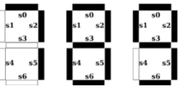
Figure 1LED images for digits 7, 8, and 9 in the seven-segment display.
4
Experimental Results
4.1
LED Data Set
For our experiments we use benchmark LED data sets generated by a program from the UCI repository [1]. The problem is to predict a digit from an image in the seven-segment display. Figure 1 shows several objects in the data set (these are “ideal images” of digits; there are also digits corrupted by noise). The seven LEDs (light emitting diodes) can be lit in different combinations to represent a digit from 0 to 9. The program generates examples with noise. There is an ideal image for each digit. An example has seven binary attributes
s0, . . . , s6 (si is 1 if theith LED is lit) and a labelc, which is a decimal digit. The program randomly chooses a label (0 to 9 with equal probabilities), inverts each of the attributes of its ideal image with probabilitypnoise= 1% independently, and adds the noisy image and the label to the data set.
4.2
Hypergraphical Assumptions for LED Data Sets
We consider two hypergraphical models that agree with the generating mechanism. These models make different assumptions about the pattern of dependence between the attributes and the label; they do not depend on a particular probability of noisepnoiseor the fact that the same value ofpnoise is used for all LEDs. For both hypergraphical structures the set of variables isV :={s0, . . . , s6, c}.
Nontrivial Hypergraphical Model. Consider the hypergraphical structure with the clustersE:={{si, c}:i= 0, . . . ,6}. A junction tree for this hypergraphical structure can be defined as a chain with verticesU :={ui:i= 0, . . . ,6}and the bijectionCui :={si, c}.
Exchangeability Model. The hypergraphical model with no information about the pattern of dependence between the attributes and the label is the exchangeability model. The corresponding hypergraphical structure has one cluster,E:={V}. The junction tree is the one vertex associated withV.
4.3
Experiments
For our experiments we create a LED data set with 10000 examples. The data are generated by the program described in section 4.1 with the probability of noisepnoise= 1%.
We consider predictors based on the signed predictability conformity measure (5). The graph with no characters on it corresponds to the idealized predictor and represents an unachievable ideal goal. In the idealized case we know the true distribution for data and use it instead of the backward kernelPσ∗in both (3) and (5). Thepure hypergraphical conformal
predictor (the graph with circles) is obtained using the nontrivial hypergraphical model both when computing p-values (3) and when computing the conformity measure (5). Analogously we use the exchangeability model to obtain thepure exchangeability conformal predictor (the
significance level
percentage of multiple predictions
0% 0.5% 1% 1.5% 2% 2.5% 3% 0% 20% 40% 60% 80%
100% pv: exch; CM: exchpv: exch; CM: hgr pv: hgr; CM: exch pv: hgr; CM: hgr pv: ideal; CM: ideal
Figure 2The final percentage of multiple predictions for significance levels between 0% and 3%. The results are for the LED data set with 1% of noise and 10000 examples.
Table 1The final percentage of multiple predictions in Figure 2 for the significance level 1% and for the graphs with squares and circles.
Seed (104) 0 1 . . . 99 Average St. dev. pv: exch; CM: hgr 0.197 0.243 . . . 0.248 0.192 0.052 pv: hgr; CM: hgr 0.203 0.244 . . . 0.250 0.196 0.049
graph with triangles point up). The twomixed conformal predictors(the graphs with squares and triangles point down) are obtained when we use different models to compute the p-values and the conformity scores. The intuition behind the pure and mixed conformal predictors can be explained using the distinction between hard and soft models made in [6]. The model used when computing the p-values (3) is the hard model; the validity of the conformal predictor depends on it. The model used when computing conformity scores (5) is the soft model; when it is violated, validity is not affected, although efficiency can suffer. The true probability distribution for our generated data conforms to both the exchangeability model and the nontrivial hypergraphical model; so all four conformal predictors are automatically valid, and we study only their efficiency. Figure 2 shows the percentage of multiple predictions Mult10000/10000 as function of the significance level ∈[0,0.03]. In the legend, the hard model used is indicated after “pv” (the way of computing the p-values), and the soft model used is indicated after “CM” (the conformity measure); “exch” refers to the exchangeability model, and “hgr” refers to the nontrivial hypergraphical model. The most interesting graph is the one with squares, corresponding to the exchangeability model as the hard model and the nontrivial hypergraphical model as the soft model. The performance of the corresponding
conformal predictor is typically better than, or at least close to, the performance of any of the remaining realistic predictors. The fact that the validity of the conformal predictor only depends on the exchangeability assumption makes it particularly valuable. The graph with triangles point down corresponds to the nontrivial hypergraphical model as the hard model and the exchangeability model as the soft model; the performance of the corresponding conformal predictor is very poor in our experiments.
Table 1 shows the percentage of the multiple prediction at the significance level 1% for two graphs (with squares and with circles) for several seeds of the pseudorandom number generator. The values of the seed are given in the units of 10,000 (so that 0 stands for 0, 1 for 10,000, 2 for 20,000, etc.). The column “Average” gives the average of all the 100 values, and column “St. dev.” gives the standard estimate of the standard deviation computed from those 100 values. The table confirms that the graphs are very close on average (see the penultimate column), but the accuracy of our experiments is insufficient to say which tends to be lower (see the last column).
5
Conclusion
The main finding of this paper is that nontrivial hypergraphical models can be useful for conformal prediction when they are true. More surprisingly, in our experiments they only need to be used as soft models; the performance does not suffer much if the exchangeability model continues to be used as the hard model. This interesting phenomenon deserves a further empirical study.
Acknowledgements We thank the COPA 2013 reviewers for comments that improved the results of the paper. We are indebted to Royal Holloway, University of London, for continued support and funding. This work has also been supported by: the EraSysBio+ grant SHIPREC from the European Union, BBSRC and BMBF; a VLA grant on machine learning algorithms; a grant from the National Natural Science Foundation of China (No. 61128003); a grant from the Cyprus Research Promotion Foundation (research contract TPE/ORIZO/0609(BIE)/24); grant EP/K033344/1 from EPSRC.
References
1 K. Bache and M. Lichman. UCI machine learning repository. School of Information and Computer Sciences, University of California, Irvine, CA, USA, 2013.
2 R. G. Cowell, A. P. Dawid, S. L. Lauritzen, and D. J. Spiegelhalter.Probabilistic Networks and Expert Systems. Springer, New York, 1999. Reprinted in 2007.
3 V. Fedorova, I. Nouretdinov, and A. Gammerman. Testing the Gauss linear assumption for on-line predictions. Progress in Artificial Intelligence, 1:205–213, 2012.
4 V. Fedorova, I. Nouretdinov, A. Gammerman, and V. Vovk. Conformal prediction under hypergraphical models. InProceedings of the Ninth International Conference on Artificial Intelligence Applications and Innovations (AIAI 2013), Paphos, Cyprus, 2013. To appear, available at www.alrw.net/articles/09.pdf.
5 V. Vovk, A. Gammerman, and G. Shafer. Algorithmic Learning in a Random World. Springer, New York, 2005.
6 V. Vovk, I. Nouretdinov, and A. Gammerman. On-line predictive linear regression. On-line Compression Modelling project (New Series), Working Paper 1, May 2005.