Trajectory tracking Sliding Mode Control for Two Wheeled Mobile Robot

2017 3rd International Conference on Electronic Information Technology and Intellectualization (ICEITI 2017) ISBN: 978-1-60595-512-4

Trajectory-tracking Sliding Mode Control

for Two-Wheeled Mobile Robot

Sizhu Cheng, Chen Liu, Chengbao Wu and Chenyao Song

ABSTRACT

According to the mechanical structure and operation principle of differential-drive two-wheeled robot, and aiming at the nonlinear systems with uncertainties variable structure, a trajectory tracking model based on sliding mode control (SMC) was designed by utilizing state vector to establish the model of system and controller. The simulating results show that robot can track line, circle and S shape trajectories well, which gave reasonable dynamic responses, adjustment performance, as well as perfect disturbance rejection. The system can eliminate errors according to the deviation from sliding surface by switching the structure of controller and is robust to external disturbance.

INTRODUCTION

Before designing a controller, the system model should be defined firstly. In reality, most systems are nonlinear, and the model is imprecise, with actual uncertainty[1][2]. From a control point of view, modeling inaccuracies can be classified into two major kinds: 1. Structured (or parametric) uncertainties, and 2. Unstructured uncertainties (or unmodelled dynamics)[3]. For any practical design, the system model must be explicitly defined[4][5]. For the class of systems to which it applies, sliding controller design provides a systematic approach to the problem of maintaining stability and consistent performance in the face of modeling imprecision[6]. It has been widely used in manipulator, ground and submarine operation vehicles, automotive transmission systems and engines, high-capacity motors and power control systems[7][8].

_______________________

1. KINETIC MODEL OF MOBILE ROBOT

Position coordinate of robot was defined by state parameters [x(t),y(t),θ(t)]T, with (x,y) gives the gravity centre and θ gives the attitude angle. Angular velocity of robot’s left and right wheel were indicated by ωL and ωR. Instead of controlling the speeds of left wheel and right wheel directly, it is possible to control the linear velocity v(t) and the angular velocity ω(t) of the robot, as show in figure 1. The kinetic equation is used to describe the relationship between speed (v(t),ω(t)) and state parameters [x(t),y(t),θ(t)]T, and the kinetic model of the wheel is obtained as followed:

) ( ) (

) ( sin ) ( ) (

) ( cos ) ( ) (

t t

t t

v t y

t t

v t x

 

 

  

 

  

(1)

DESIGN OF TRAJECTORY TRACKING CONTROLLER

Control Requirements

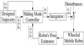
The trajectory of the robot is controlled by cascade control, in which the outer loop adopts sliding mode control, and the inner loop uses PID control. Figure 2 is the general control scheme of SMC loop.

Now considered the single-input system as followed:

u y x b y x f y x

 

   

 

  

 

) , , ( ) , ,

(  



(2)

u indicated the output control signal of the controller [v(t) ω(t)]T in figure 2, which including torque signal of wheel. Function f(x,y,θ) and b(x,y,θ) are imprecise, and there are many sources of uncertainties[9][10]. In figure 2, [xd,yd,θd]T indicates the desired position coordinate of the trajectory would be

tracked. The control design that should be taken into consideration in reality, is when model f(x,y,θ) and b(x,y,θ) containing uncertainties, actual state [x,y,θ]T can still track specific time-varying desired state [xd,yd,θd]T. This

assumption can be detailed implemented by designing a robust controller including SMC and PID control, and the controller should output control signal vector [vc,ωc]T before disturbances, as shown in figure 2. In a second

Design Sliding Mode Controller

Figure 1. Two-wheeled differential-drive robot with state parameters (x,y,θ)T.

Figure 2. General control scheme of SMC loop.

In figure 2, the state vector of robot [xr,yr,θr]T was defined by real position

vector at the next moment, and error vector was defined as [xe,ye,θe]T =

[xd,yd,θd]T - [xr,yr,θr]T. (vr(t),ωr(t)) indicates the real line velocity and angular

velocity at the next moment of the robot. Therefore, the error vector of trajectory tracking should be:

                                   d r d r d r d e e e y y x x y x      

 0 0 1 0 cos sin -0 sin cos d d d (3)

Differentiate the upper forms and substituted into function (3):

d r e d e e r e d e e r d e t x v y y v v x                    ) ( ) sin( ) cos(    (4)

[vd ωd]T is the desired velocity control signal that input to sliding mode controller. The following sliding surfaces are proposed:

e e kx

x

| | ) sgn( 0 2

2 ye k ye k ye e

s      (6)

s s V  T

2 1

is the Lyapunov function candidate[12], and

2 2 1 1 2 2 2 2 1 1 1 1 2 2 1 1 )) sgn( ( )) sgn( ( s P s P s Q s V s s Q s s s Q s V s s s s V

T _{     }

                     (7)

As V is negative semi-definite function, it is sufficient to choose Qi and Pi such that Qi·Pi≥0[13]. The above formulas are simultaneously and mathematically transformed, the final control signal output by the controller should be: ) cos( ) sin( ) sgn( 1 1 1 e d e e r d e d e e c v v y y x k s P s Q v         

        (8)

 

 

 (9)

SIMULATIONS

SMC loop translated variables vc and ωc to PID loop, and PID loop

feedback ωr, vr, xr, yr ,θr signals to SMC loop.

Straight Line Trajectory

The positions of the virtual and actual robot are shown in figure 3. For the desired signal, only the X direction of the trajectory increases, which gives a straight line trajectory, and the desired distance was 1.7m. The real output is deflected slightly with the largest error less than 20×10-3, and the result was reasonably. The error reached the maximum at 1.5m, and then decreased.

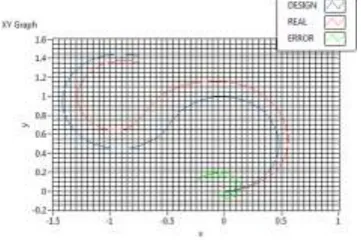
Circle Trajectory

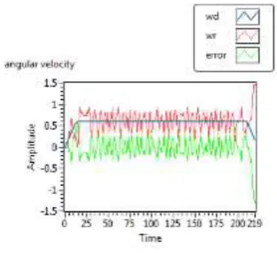
The positions of the virtual and actual robot are shown in figure 4. The input desired trajectory is a circle with a radius of 1m, and the robot actually runs three cycles. From figure 4b), it can be found that at the beginning the error is zero while keep increasing. The largest error of circle trajectory was about 0.12m, and the error was steady, which was steady-state error. The reason of the steady-state error can be seen from the desired and real linear and the angular velocities with error in figure 5. In figure 5b), the angular velocity of the robot had obvious oscillation, while there was no steady-state error. However, in figure 5a), the linear velocity had steady-state error all the time and lager than the desired velocity of input control signal, which led to the radius of real trajectory larger than the desired one. Although steady-state error and oscillations exists, the linear and angular velocities are stable, the system is still robust to resist the disturbance in actual operation.

a) Position of the virtual and actual robot. b) Error between the virtual and actual robot. Figure 4. Position of the virtual and actual robot (m).

a) Linear velocities with error (m/s) b) Angular velocities with error (rad/s)

S trajectory

The positions of the virtual and actual robot are shown in figure 6. The desired trajectory began from (0,0), and the curvature of S shape was 2m-1. In actual operation, the robot crossed the first arc with the curvature was 1.67m-1, the second curves was 1.54m-1, the third curves was 3.33m-1, the fourth curves was 2.5m-1, and the fifth curves was 2.22m-1. In figure 6, the green error line shows that the maximum position error was about 0.2m, and the maximum curvature error was 1.33m-1. Substantially, the output trajectory was in parallel with the input one, which was the steady-state error. The actual curvature radius of the first half section was less than the set value, and the actual curvature radius of the second half segment was greater than the set value. In addition, the actual running track was always on the right side of the setting trajectory. This phenomenon indicated that there was no oscillation of the system when the trajectory was self-correcting. Besides, the error reached the maximum in the middle of the route. The error from the first arc to the middle section was an increasing process, and the error between the middle and the end was a decreasing process, which meant the system had the ability to correct itself.

Figure 6. Position of the virtual and actual robot(m).

CONCLUSIONS

According to the simulation results, the conclusions are summaries as below:

1. Robot can track the desired input signal well under the robust control with sliding mode controller, and the simulation of the straight line trajectory was the best one;

2. The real trajectories were stable, while the output linear and angular velocities had slight oscillations. Oscillation was caused by the coupling of variables, the noise of the hardware and the interference of the external environment, which cannot be completely eliminated.

ACKNOWLEDGEMENT

This project was financially supported by the National Natural Science Foundation of China (No. 51575117 and 61179051).

REFERENCES

1. Liu Y J, Tong S C. Adaptive fuzzy control via observer design for uncertain nonlinear systems with unmodeled dynamics[J]. IEEE Transactions on Fuzzy Systems: Vol.21 (2), pp.275- 288, 2013.

2. Qi Dong-Lian, Wang Qiao. Comparison between two different sliding mode controllers for a fractional-order unified chaotic system[J]. Chinese Physics B, Vol.20 (10), pp.100505 (9pp), 2011.

3. Lennart Ljung. System identification: Theory for the user[M]. Prentice Hall: 2 edition, 1999.

4. Ngongi W, Du J, Mohamed A. Relaxed LMI Stability Conditions Based Fuzzy Control Design for Dynamic Positioning of Ships[D]. Journal of Advanced Shipping and Ocean Engineering, 2013.

5. Jean Pierre Barbot. Sliding Mode Control in Engineering[M]. Dekker, 2007.

6. Kenichiro Nonaka, Takatsugu Oda. Model Predictive Sliding Mode Control for Four Wheel Steering and Driving Vehicles[J]. IFAC Proceedings Volumes: Volume 46, Issue 21, Pages 794-799, 2013.

7. S. Dhar, P.K. Dash. A new backstepping finite time sliding mode control of grid connected PV system using multivariable dynamic VSC model[J]. International Journal of Electrical Power and Energy Systems, Volume 82, Pages 314-330, 2016.

8. Mohammad Amin Alandi Hallaj, Nima Assadian. Sliding Mode Control of Electromagnetic Tethered Satellite Formation[J]. Advances in Space Research, Volume 58, Issue 4, Pages 619-634, 2016.

9. Fu Jun Wang, Xing Yu Zhao. Modeling of a Direct-Drive Table for Automatic Wire Bonder[J]. Key Engineering Materials, Volumes 467-469, Pages 1315-1318, 2011. 10. Jun Liu, Pu Guo Gui. Structure Optimization of the Aluminum Alloy Frames of Flight

Simulator[J]. Key Engineering Materials. Volume 667, 582-587, 2015.

11. Sang-Myeong Kim, Michael J. Brennan. Narrowband feedback for narrowband control of resonant and non-resonant vibration[J]. Mechanical Systems and Signal Processing. Volumes 76–77, Pages 47-57, 2016.

12. Yuangong Sun. Stability analysis of positive switched systems via joint linear copositive Lyapunov functions[J]. Nonlinear Analysis: Hybrid Systems. Volume 19, Pages 146-152, 2016.